Stixel Based Scene Understanding for Autonomous Vehicles

      

City, University of London Institutional Repository

Citation

:

Wieszok, Z., Aouf, N., Kechagias-Stamatis, O. and Chermak, L. (2017). Stixel

Based Scene Understanding for Autonomous Vehicles. 2017 IEEE 14th International

Conference on Networking, Sensing and Control (ICNSC), pp. 43-49. doi:

10.1109/ICNSC.2017.8000065

This is the accepted version of the paper.

This version of the publication may differ from the final published

version.

Permanent repository link:

http://openaccess.city.ac.uk/22107/

Link to published version

:

http://dx.doi.org/10.1109/ICNSC.2017.8000065

Copyright and reuse:

City Research Online aims to make research

outputs of City, University of London available to a wider audience.

Copyright and Moral Rights remain with the author(s) and/or copyright

holders. URLs from City Research Online may be freely distributed and

linked to.

City Research Online:

http://openaccess.city.ac.uk/

[email protected]

0F

Abstract—We propose a stereo vision based obstacle detection and scene segmentation algorithm appropriate for autonomous vehicles. Our algorithm is based on an innovative extension of the Stixel world which neglects computing a depth map. Ground plane and stixel distance estimation is improved by exploiting an online learned color model. Furthermore, the stixel height estimation is leveraged by an innovative joined membership scheme based on color and disparity information. Stixels are then used as an input for the semantic scene segmentation providing scene understanding, which can be further used as a comprehensive middle level representation for high-level object detectors.

Index Terms—Dynamic Programming, Obstacle Detection, Stereo Vision, Semantic Segmentation, Stixel World

I. INTRODUCTION

n intelligent vehicle consists of many subsystems that are responsible of controlling the complicated process of autonomous driving and navigation. However, obstacle detection and scene understanding are the most critical parts of the system on which the passenger’s and vehicle’s safety rely on. Out of many available obstacle detection systems [1], in this paper we extend the promising Stixel World [2]. The latter representation is a particular scene tessellation which divides the scene into a set of rectangular sticks named “stixels”. Each stixel provides information of the 3D position and height of the obstacle along with the available free-space.

Although the Stixel World algorithm originally proposed by Badino et al. [2] is able to achieve real-time performance, it requires dedicated FPGA hardware to apply the Semi-Global Matching algorithm in order to obtain a dense depth map. A processing efficient solution is proposed by Benenson et al. [3] which allows stixel estimation without a depth map. In that case, even though the speedup is substantial, accuracy is downgraded compared to the original method.

This work introduces a number of innovations compared to [3] achieving better accuracy while still neglecting the requirement of a dense depth map. In specific, ground plane estimation is improved by using an online learned color model which reduces the estimation error by a factor of two compared to [3]. In addition, the color road model is used to advance the stixel distance estimation and reduce the number of erroneously detected obstacles while it maintains

Authors are with the Signals and Autonomy Group. Centre for Electronic Warfare Information and Cyber, Cranfield University at the UK Defence Academy, Shrivenham, SN6 8LA, UK (e-mail: {Z.Wieszok, n.aouf o.kechagiasstamatis, l.chermak}@cranfield.ac.uk)

the missed obstacle ratio. Height estimation is enhanced by combining disparity information with color cues.

Finally, our work takes advantage of this middle-level stixel representation and proposes semantic segmentation for scene understanding distinguishing pedestrians and vehicles from infrastructure and vegetation. This segmentation can be used as input to a high level appearance-based detector for precise classification with a significantly reduced search space.

II. RELATED WORK

Stereo systems are extensively used in the context of obstacle detection algorithms. Bernini et al. [1] proposes to categorize the algorithms into four groups. One of these is the occupancy grids algorithm which is further extended into the Stixel World [2]. A number of approaches are undertaken to improve the Stixel World representation [4]– [6] with an important enhancement utilizing the online color modelling for the road versus obstacle segmentation [7], [8]. The stixel estimation can be also be leveraged by using pixel level semantic segmentation based on color cues and the geometric properties of the scene [9]. That approach is further extended utilizing convolutional neural networks [10].

Scharwächter et al. in [11] have proposed a multi-cue scene segmentation. Initially, the algorithm generates hypotheses for object regions using a multilayer Stixel World [12], which are then joined to obtain larger regions using DBSCAN [13] clustering. Then depth and height cues are integrated into the region descriptors introducing a bag of depth features. Lately, a multi-class SVM algorithm is used to classify regions into five semantic classes [14] which is further developed to provide spatial and temporal coherence for a semantic class label. The temporal coherence is ensured via a Hidden Markov Model and a Kalman filter is applied for the velocity estimation. Spatial filtering is performed through a Conditional Random Field to ensure global smoothness of the labels.

Stixel Based Scene Understanding for Autonomous Vehicles

Zygfryd Wieszok, Nabil Aouf, Odysseas Kechagias-Stamatis and Lounis Chermak

A

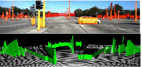
Fig 1. Stixel representation in camera image. Bottom image presents stixel representation in reference to laser data (best seen in color)

2017 IEEE 14th International Conference on Networking, Sensing and Control (ICNSC) Calabria, Italy, 16-18 May 2017

DOI: 10.1109/ICNSC.2017.8000065

© 2017 IEEE. Personal use of this material is permitted. Permission from IEEE must be obtained for all other uses, in any current or future media, including reprinting/republishing this material for advertising or promotional purposes, creating new collective works, for resale or redistribution to servers or lists, or reuse of any copyrighted component of this work in other

[image:2.612.315.559.147.262.2]

III. STIXEL ESTIMATION

The proposed stixel estimation algorithm extends [3] and includes five processing steps. Initially, the pixel-wise cost volume is computed from rectified stereo images. Then, the color model is trained for the road segmentation and the cost volume is used to estimate the ground plane, which in turn is used to estimate the stixel disparities. Finally, the stixel’s disparity and color are used to estimate the stixel height. Throughout this paper we assume a stixel width of one pixel. A. Cost volume computation

Given a pair of rectified stereo images, the matching cost volume is computed: for every pixel in the left image and every disparity value, the matching cost with the corresponding right image is calculated. The matching cost is computed as the vanilla sum of absolute differences over the RGB color channels:

( , ) ( , )

( , , ) l r

m

I u v I u d v c u v d

channels

 

 (1)

where 𝐼𝑙 and 𝐼𝑟 are the rectified left and right images,

𝑐ℎ𝑎𝑛𝑛𝑒𝑙𝑠 represents the number of color channels and u,v,d represent the column, row and disparity in respect.

B. Road probability

Assuming a road environment and a fixed camera set-up, the road probability Pr(u,v) at certain locations within the

image is computed (Fig. 2 (a)). Then we use Pr(u,v) to

generate a training mask for the online learning color model that is needed for the road segmentation. The training mask presented in Fig 2 (b) is based on:

r

1 P ( , ) 0.92 ( , )

0

tm

u v

I u v

otherwise

 

 

 (2)

C. Online learned color model

Road pixel information in the input image can successfully leverage the estimation quality of the ground plane and stixel disparity. This paper introduces an online learned color model (OLCM) for road segmentation inspired by [7]. In specific, the color model is constructed as a 2D normalized histogram computed within the training mask ( Fig

3

(a)). The histogram is based on the HSV color space and utilizes the hue and saturation channels which are discretized into 60x60 equally spaced bins. In order to obtain the road segmentation, the histogram is back projected onto the left and right input image, resulting in the probability for each pixel belonging to the road as 𝑃𝑙𝑟(𝑢, 𝑣) and 𝑃𝑟𝑟(𝑢, 𝑣) in

respect. A road segmentation example is presented in Fig. 3 (b).

D. Ground plane estimation

We estimate the ground plane by exploiting the v-disparity representation [16]. The latter, is a summed pixel cost of the unidimensional slice of the cost volume as it is projected along the horizontal u-axis. Then the ground plane parameters are found by fitting a line to the low cost regions of the v-disparity image. Although it is assumed that the road is a dominant surface within the image, there are cases where this assumption is violated and the low cost regions in the v-disparity image are misplaced (Fig 4 (b)).

In this work we overcome this problem by weighting the contribution of each pixel onto the v-disparity image based on the probability of the pixel being the road which is obtained using OLCM. The algorithm is expressed as:

| |

0

( , ) ( , , ) ( , , )

U

v m

u

I_ d v P u v d c u v d







 (3) where P u v d( , , )P ( , ) P ( , ) P (_r u v  _lr u v  _rr ud v, ).

The improvement of the ground estimation can be clearly seen in Fig 4 (c) where the line is consistently on the low cost regions, comparing to original algorithm depicted in Fig 4 (b).

E. Stixel distance estimation

The projection of the cost volume along the horizontal axis assists in ground estimation, while the projection along the vertical (v-axis) provides an estimation of the stixel’s distance.

Following the approach of Kubota et al. [17], the depth of the stixel is estimated using 2D dynamic programming over a data term 𝑐𝑠 and a smoothness term 𝑠𝑠. The goal is to find

the optimal disparity for each stixel by optimizing the following equation:

( )

*

,

( ) arg min ( , ( )) ( ( ), ( ))

d u _{a b}

S s s a b

u u u

d u 



c u d u 



s d u d u (4)

where ua and ub are neighboring columns within the scene.

The 2D minimization problem is solved using dynamic programing in the u-disparity domain.

E.1 Data term

In [17] the stixel cost cs(u,d) defines whether a stixel is

present in the image column u and comprises of the stixel cost co(u,d) and the ground cost cg(u,d). In our work we add

an additional probability term cp(u,d) and the stixel cost

becomes:





( , ) ( , ) ( , ) ( , )

s o g p

c u d  c u d c u d c u d (5)

[image:3.612.56.555.66.124.2]

(a) (b) (a) (b)

Fig 2. (a) road probability, the darker the pixel color the lower the probability the pixel belongs to the road (b) corresponding training mask.

with ( ) ( , ) | | ( ) ( ) r ( , ) ( , ) ( , , ) ( , ) ( , , ( ))

P ( , ) ( , ) ( , ) 1

( , ) ( ) o

o

v d

o m

v v h d V

g m ground v v d

v d

lr v v h d

p

o

c u d c u v d

c u d c u v f v

u v P u v c u d

v h d v d

        







(6)

where v(d) remaps a disparity value to the image row based on the ground plane estimation, v(ho,d) is the upper

boundary of the object given by the disparity and height ho,

which is computed using the ground plane estimate and the camera calibration, and finally fground(v)=v-1(d).

The innovative probability term cp(u,d) suggested is

calculated based on the probability of the road obtained using the OLCM. cp(u,d) encodes the reliance that the higher

the probability of the road the more unlikely that the object of minimum height ho is present at distance 𝑑. The estimated

stixels with a fixed height are shown in Fig 5. E.2 Smoothness term

In a stereo system, some of the objects visible in the left image are occluded in the right image and vice versa. While processing the left image, any stixel behind the “one disparity less per pixel to the left” [17] should be invalidated by the occlusion constraint. This constraint is ensured by the smoothness term:

, 1

( , ) ( , ) 1

0, 1

a b s a b o a b a b a b

d d

s d d c u u d d

d d      _    _{ }  (7)

where da=d(ua) and db=d(ub) with ua one pixel left of the

pixel ub. The 𝑠𝑠= ∞ case ensures that no stixel distance

violates the occlusion constraint. F. Stixel height estimation

The actual height of each stixel is estimated as the likelihood of each pixel above the ground belonging to the estimated stixel disparity 𝑑𝑠∗(𝑢). The likelihood is expressed

by the membership function m u v( , )m u v_d( , )m u v_c( , ), where:



1



( , ) 2 max(0, ( , )) 0.5

d

m u v   m u v  (8)

* * 2 1 * ( ( )) ( ( , , ), ( , , ( )) ( , ) ( ( )) S

m m S

d N d u S

m c u v d c u v d u m u v

N d u







(9)

* * max max * 2 _* max max

max(| |, )

( , )

max(| |, )

c c

c c

m c c

c c otherwise       _        _  (10)

and cm(u,v,da) is the local minimum of the cost function for a

pixel at location (u,v) in the image belonging to disparity da,

N(da) indicates a small neighbourhood around 𝑑𝑎 (e.g. ±5

pixels), |N(da)| indicates the number of elements in 𝑁(𝑑𝑎),

∆𝑚𝑎𝑥 is a small constant (this paper assumes ∆𝑚𝑎𝑥= 10) and

𝑐̃𝑚 is the cost value after applying a 5x5 mean filter.

( , ) [ 1,1]

d

m u v   where 1 means full membership, -1 means no membership and 0 indicates no contribution. We improved height estimation by extending the disparity membership [3] by introducing an innovative color membership function mc(u,v). In order to obtain mc, we

construct the color histogram within a rectangle R with

coordinates * *

0

1 1

, ( ( )), , ( , ( ))

2 S 2 S

w w

R u_   v d u u  v h d u _

  in the

following order: column and row of left bottom corner, column and row of upper right corner. The parameter 𝑤 is the column window which is set to 5. Fig. 6 shows an example on the suggested stixel height estimation concept. F.1 Data term

The membership function m(u,v) is then converted into a height cost ch(u,v):

* max

*

( , ( ))

( )

( , ) | ( , ) 1| | ( , ) 1|

S

bottom

v h d u v

h

w v w v u

c u v m u v m u v

 





 



 (11)

where 𝑣(ℎ_𝑚𝑎𝑥, 𝑑_𝑠∗(𝑢)) indicates the top row of the object of height ℎ_𝑚𝑎𝑥 at disparity 𝑑_𝑠∗(𝑢) and *

( )

bottom

v u denotes the bottom boundary of the stixel.

F.2 Smoothness term

The smoothness term is defined as:

* *

1

2

( ( )) ( ( ))

( , , ) | | max 0.1 s a s b

h a a b b a b

z d u z d u s u v u v k v v

z        _  _    (12)

(a) (a) (b)

(b) (c) (c) (d)

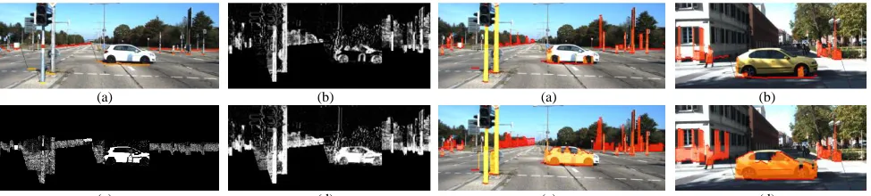
[image:4.612.54.280.52.161.2]

Fig 4. (a) Example input image (b) corresponding v-disparity representation using original algorithm (c) proposed method (best seen in color)

[image:4.612.320.558.52.161.2]

where 𝑘1 is a scaling factor that penalizes the top shapes that

are non-horizontal (set to 1) and ∆𝑧2 the minimum distance

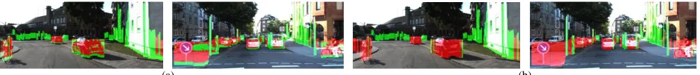
of adjacent stixels that influence each other (set to 3m). Fig. 7 compares the height estimation using the original algorithm and the modified version introduced in this paper. It can be clearly seen that color information enhances the stixel height estimation in texture-less and shiny regions like a car or building facades.

IV. STIXEL SEMANTIC SEGMENTATION

This paper proposes a two stage process to classify a stixel into two commonly encountered classes: the vegetation and infrastructure (V&I) and the car and pedestrian (C&P). First, a semantic class is assigned to every pixel within the stixels boundaries and then the semantic class is assigned to each stixel, based on the dominant class within that stixel. This approach ensures classification consistency.

The pixel level classification is based on a feature vector constructed from 13 features divided into 3 categories namely: color, texture and geometric features. Pixels are classified using the Decision Tree classifier trained in RapidMiner Studio.

A. Color features

Color pixel features are extracted on two color spaces, the CIELab and the YCrCb. The color components of the former space are denoted as 𝐼_𝐿𝑎𝑏𝑘 (𝑢, 𝑣) where 𝑘 ∈ {𝐿, 𝑎, 𝑏}. From the latter colour space two channels are used, the Cr and Cb,

which are denoted as 𝐼_{𝑌𝐶𝑟𝐶𝑏}𝐶𝑟 and 𝐼_{𝑌𝐶𝑟𝐶𝑏}𝐶𝑏 . These two channels of the YCrCb space provide illumination invariance.

B. Texture features

We extract simplified texture information from the local color homogeneity proposed in [18] consisting of the color standard deviation Φk _{and the discontinuity values E}k_:

( , ) 1 ( , ) ( , )

k k k

H u v  E u v  u v (13)

where

max max

( , ) ( , )

( , ) , ( , )

k k

k k

k k

u v e u v

u v E u v

e





   (14)

The first feature is expressed as the color standard deviation in the CIELab space:





1 1

2 2

2

1 1

2 2

1

( , ) ( , ) ( , )

w w u v

k k k

Lab w w m u n v

u v I m n m n

w

 

 

 

 

   



 

 (15)

1 1

2 2

2

1 1

2 2

1

( , ) ( , )

w w u v

k k

Lab w w m u n v

u v I m n

w



 

 

 

   



 

(16)

where 𝑤 defines a window size set to 5. The second feature represents the discontinuity in the color component

( , )

k Lab

I m n which is represented by an edge value based on the Sobel edge detector. The normalized edge magnitude

𝑒𝑖𝑗𝑘 (𝑘 = 𝐿, 𝑎, 𝑏) of the gradient at location (𝑖, 𝑗) is given by:

2 2

( , ) ( , ) ( , )

k k k

x y

e u v  G u v G u v (17)

where 𝐺_𝑥𝑘 and 𝐺_𝑦𝑘 are the gradients of the color component in the CIELab space in the 𝑥 and 𝑦 direction respectively. The kernel size for the Sobel operator is set to 5 and for computational consistency the standard deviation of the color is computed within a window of size 5x5.

C. Geometric features

We extract two geometric features, the first being the height above the ground defined as ℎ𝑔(𝑢, 𝑣). This feature

encodes the vertical position of the object based on the fact that objects are physically located on the top of the supporting ground plane. The second feature is a height of the stixel labelled as ℎ_𝑠(𝑢) which is the difference between the top and bottom border.

D. Stixel classification

The special coherence of the segmentation is ensured by relying segmentation in stixels rather than pixels. Based on the assumption that a single stixel describes only one object, all pixels within this particular stixel belong to the same object. The class assigned to each stixel is based on the dominant class within each stixel.

Classification examples are presented in Fig. 8 and clearly show that the stixel-level classification is superior compared to the pixel-level.

(a) (b) (a) (b)

(c) (d) (c) (d)

[image:5.612.61.548.64.174.2]

Fig 6. (a) input image with outlined bottom stixel border, (b) disparity membership 𝒎𝒅(𝒖, 𝒗); (c) colour membership 𝒎𝒄(𝒖, 𝒗); (d) joined membership 𝒎(𝒖, 𝒗) (best seen in color)

[image:5.612.323.559.245.341.2]

V. EXPERIMENTS A. Ground estimation

We challenge our proposal on the Kitti stereo benchmark [19] against the stixel approach suggested by Benenson et al. [3]. The Kitti stereo benchmark includes 200 stereo images with a reference disparity map obtained by an accurate laser scanner that has depth estimation with centimeter accuracy.

First trial concerns the ground plane error estimation which is measured based on:





2

0 0

1 2

| ( ) ( ) | ( ) ( )

,

| | | |

D D

r e r e

d d

norm norm

v d v d v d v d

L L

D D

 

 

 









(18) where 𝑣𝑟(𝑑) is the reference ground line, 𝑣𝑒(𝑑) is the

estimated ground line in the v-disparity image based on the matching cost and |𝐷| is a maximum disparity which in this work is set to 128.

The reference ground line is estimated using the Labayrade’s algorithm [16] but instead of using Semi-Global Matching [20] for the depth estimation, we exploit the reference disparity maps from the Kitti stereo benchmark in order to avoid errors of the disparity estimation algorithm.

Table I presents the average ground plane error estimation on the entire Kitti database which shows that our proposal is more than twice accurate compared to [3].

B. Distance estimation

In this trial we evaluate the proposed stixel distance estimation compared to the reference disparity maps provided in the Kitti stereo benchmark [19]. Therefore, stixels are converted into the corresponding disparity map:

, ( ) ( , )

( , ) ( ) ( )

1, ( , )

bottom o sd ground bottom

o

d v u v v h d

I u v f v v u v

v h d v   



 

  



(19)

The disparity across the stixels is constant as it assumes vertical obstacles, although some objects do not fully match this condition. To minimize this effect the stixel height is restricted to 80cm as proposed in [21].

The error between the reference 𝐼𝑑 and the stixel disparity

map 𝐼_𝑠𝑑 is calculated as: ( , ) ( , )

( , ) 0 ( , ) 0 ( , )

( , )

0 ( , ) 0 ( , ) 0

sd d

d sd d

d sd

I u v I u v

I u v I u v

I u v e u v

I u v I u v



 _{  }

  

 _{  }



(20)

The error is normalized using the reference disparity, in order to make the magnitude the of error uninfluenced by the distance. Depending on the sign of the error e(u,v), the stixel error is classified into a false positive FP error for mistakenly detected obstacles and a false negative FN error for missed obstacles. An example of error classification is depicted in Fig. 9 where red color depicts FP and blue color represents FN errors.

Fig. 10 and Fig. 11 illustrate the number of FP and FN pixels in respect, in relation to the distance to the autonomous vehicle. Both figures indicate that the proposed extensions reduce the number of FP pixels by minimizing the amount of mistakenly detected obstacles while the amount of FN is maintained.

C. Semantic segmentation

We further evaluate our proposed solution in the context of scene understanding using the semantic dataset proposed by Xu et al. [22]. This dataset provides 70 training and 39 test labelled images. Tables II and III present the classification results in a confusion matrix form for the pixel and stixel level in respect. The ground truth for the pixel-level classification is obtained directly from the semantic dataset while for the stixel-level classification by applying Eq. 18 on the pixel-level ground truth.

Table II shows that the pixel-level classification can be significantly improved ensuring spatial coherence, by assigning a single class for a stixel. The results for the stixel-level classification (Table III) demonstrate a significant improvement providing an overall accuracy of 88.2%. It can be noticed that the recall and precision for both classes are considerably improved. In addition, it is worth noticing that the number of classified stixels is significantly smaller than the number of classified pixels. This reveals that stixel representation considerably reduces the amount of data while affording high accuracy.

VI. CONCLUSION

We propose an enhanced stixel estimation that neglects the computation of a processing deficient depth map, while in parallel affords high accuracy. This is achieved by exploiting an online learned color model which is used for ground plane and stixel distance estimation. The suggested method for ground plane estimation reduces the error by more than a factor of two, while the suggested stixel distance estimation reduces the FP and maintains the FN compared to current proposals.

(a) (b)

[image:6.612.60.562.64.118.2] [image:6.612.58.295.279.326.2]

REFERENCES

[1] N. Bernini, M. Bertozzi, L. Castangia, M. Patander, and M. Sabbatelli, “Real-time obstacle detection using Stereo Vision for Autonomous Ground Vehicles: A Survey,” in 17th International IEEE Conference on Intelligent Transportation Systems (ITSC). Qingdao, China, 8 October, 2014, no. 1, pp. 873–878.

[2] H. Badino, U. Franke, and D. Pfeiffer, “The Stixel World - A Compact Medium Level Representation of the 3D-World,” in Lecture Notes in Computer Science), 2009, vol. 5748, pp. 51–60. [3] R. Benenson, R. Timofte, and L. Van Gool, “Stixels estimation

without depth map computation,” Proc. IEEE Int. Conf. Comput. Vision. Barcelona, Spain, 6 Novemb., pp. 2010–2017, 2011. [4] D. Pfeiffer, S. Gehrig, and N. Schneider, “Exploiting the power of

stereo confidences,” in Proceedings of the IEEE Computer Society Conference on Computer Vision and Pattern Recognition, 2013, pp. 297–304.

[5] D. Pfeiffer and U. Franke, “Efficient representation of traffic scenes by means of dynamic stixels,” in IEEE Intelligent Vehicles Symposium, Proceedings, 2010, pp. 217–224.

[6] M. Muffert, N. Schneider, and U. Franke, “Stix-fusion: A probabilistic stixel integration technique,” in Proceedings - Conference on Computer and Robot Vision, CRV 2014, 2014, vol. 1, no. c, pp. 16–23.

[7] W. P. Sanberg, G. Dubbelman, and P. H. N. de With, “Extending the Stixel world with online self-supervised color modeling for road-versus-obstacle segmentation,” in 17th IEEE International Conference on Intelligent Transportation Systems, 2014, pp. 1400– 1407.

[8] W. P. Sanberg, G. Dubbelman, and P. H. N. De With, “Color-Based Free-Space Segmentation Using Online Disparity-Supervised

Learning,” in IEEE Conference on Intelligent Transportation Systems, Proceedings, ITSC, 2015, vol. 2015-Octob, pp. 906–912. [9] T. Scharwachter and U. Franke, “Low-level fusion of color, texture

and depth for robust road scene understanding,” in IEEE Intelligent Vehicles Symposium, Proceedings, 2015, vol. 2015-Augus, no. Iv, pp. 599–604.

[10] E. Levi, Dan and Garnett, Noa and Fetaya, “StixelNet: A Deep Convolutional Network for Obstacle Detection and Road Segmentation,” in Proceedings of the British Machine Vision Conference (BMVC), 2015, pp. 1–12.

[11] T. Scharwachter, M. Enzweiler, U. Franke, and S. Roth, “Efficient multi-cue scene segmentation,” in Lecture Notes in Computer Science, 2013, vol. 8142 LNCS, pp. 435–445.

[12] D. Pfeiffer and U. Franke, “Towards a Global Optimal Multi-Layer Stixel Representation of Dense 3D Data,” in Procedings of the British Machine Vision Conference 2011, 2011, pp. 51.1–51.12. [13] M. Ester, H.-P. Kriegel, J. Sander, and X. Xu, “A Density-Based

Algorithm for Discovering Clusters in Large Spatial Databases with Noise,” in Proc. KDD, 1996, pp. 226–231.

[14] T. Scharwächter, M. Enzweiler, U. Franke, and S. Roth, “Stixmantics: A medium-level model for real-time semantic scene understanding,” in Lecture Notes in Computer Science, 2014, vol. 8693 LNCS, no. PART 5, pp. 533–548.

[15] J. Fritsch, T. Kuhnl, and A. Geiger, “A new performance measure and evaluation benchmark for road detection algorithms,” 16th Int. IEEE Conf. Intell. Transp. Syst. (ITSC 2013), no. Itsc, pp. 1693– 1700, 2013.

[16] R. Labayrade, D. Aubert, and J.-P. Tarel, “Real time obstacle detection in stereovision on non-flat road geometry through ‘v-disparity’ representation,” in Intelligent Vehicle Symposium, 2002. IEEE, 2002, vol. 2, pp. 646–651.

[17] S. Kubota, T. Nakano, and Y. Okamoto, “A Global Optimization Algorithm for Real-Time On-Board Stereo Obstacle Detection Systems,” in Proc. IEEE Intelligent Vehicles Symposium, 2007, pp. 7–12.

[18] X.-Y. Wang, T. Wang, and J. Bu, “Color image segmentation using pixel wise support vector machine classification,” Pattern Recognit., vol. 44, no. 4, pp. 777–787, 2011.

[19] M. Menze and A. Geiger, “Object scene flow for autonomous vehicles,” in Proceedings of the IEEE Computer Society Conference on Computer Vision and Pattern Recognition, 2015, vol. 07–12-June, pp. 3061–3070.

[20] G. Heiko Hirschmüller, “Accurate and Efficient Stereo Processing by Semi-Global Matching and Mutual Information,” in Computer Vision and Pattern Recognition, 2005. CVPR 2005. IEEE Computer Society Conference on (Volume: 2), 2005, pp. 807 – 814.

[21] D. Pfeiffer, S. Morales, A. Barth, and U. Franke, “Ground truth evaluation of the Stixel representation using laser scanners,” in 13th International IEEE Conference on Intelligent Transportation Systems, 2010, pp. 1091–1097.

[22] P. Xu, F. Davoine, J.-B. Bordes, H. Zhao, and T. Denoeux, “Information Fusion on Oversegmented Images: An Application for Urban Scene Understanding,” in Thirteenth IAPR International Conference on Machine Vision Applications, 2013, pp. 189–193.

(a) (b) (c) (d)

[image:7.612.55.556.53.229.2]

Fig 9. (a) stixels estimation (b) reference disparity map (c) stixel disparity map (d) stixel error (best seen in color)

Fig 10. FP classified pixels as belonging to an obstacle Fig 11. FN classified obstacle pixels 0 10000 20000 30000 40000 5

.3 ₅.7 ₆.0 ₆.4 .9_{6 7}.4 ₈.0 ₈.7 ₉.6

1 0 .7 1 2 .0 1 3 .7 1 6 .0 1 9 .2 2 4 .0 3 2 .0 4 8 .0 9 6 .1 N u mb er o f er ro n eu s p ix el s

Distance from vehicle (m) Benensen et al. [12]

OLCM for ground plane

OLCM for ground plane and stixel distance 0 10000 20000 30000 40000 50000 60000 2

.2 ₂.4 ₂.5 ₂.8 ₃.0 ₃.2 ₃.5 ₃.7 ₄.0 ₄.4 ₄.9 ₅.4 ₆.1 ₇.0 ₈.2 ₉.9

1 2 .4 1 6 .7 2 5 .6 5 4 .9 N u mb er o f er ro n eu s p ix el s

Distance to vehicle (m) Benensen et al. [12]

OLCM for ground plane

OLCM for ground plane and stixel distance

TABLE I

GROUND PLANE ESTIMATION ERROR

Ground estimation Error L1norm Error L2norm

Benenson et al. [3] 3.847 5.708

Our proposal 1.770 2.600

TABLE II

CONFUSION MATRIX FOR PIXEL LEVEL CLASSIFICATION

Accuracy: 78.360% Actual value

PRECISION V&I C&P

Predicted value

V&I 1645595 191697 89.57% C&P 373584 401387 51.79% RECALL 81.50% 67.68%

TABLE III

CONFUSION MATRIX FOR STIXEL LEVEL CLASSIFICATION

Accuracy: 88.180% Actual value

PRECISION V&I C&P

Predicted value

V&I 30497 791 97.47% C&P 4060 5691 58.36% RECALL 88.25% 87.80%

[image:7.612.94.550.208.745.2]