A diagrammatic analysis of the variational perturbation method for classical fluids

(1)

A diagrammatic analysis of the variational

perturba-tion method for classical fluids

†

Leo Luea

The statistical mechanics of classical fluids can be approached from the particle perspective, where the focus is on the various positions and interactions of the particles, and from the field perspective, where the focus is on the form of the interaction fields generated by the particles. In this work, we combine these two perspectives by examining the variational perturbation method for classical fluids, which has been widely used to describe nonuniform electrolyte systems. Most of this work has been for low orders of the approximation, it has been limited to cases where the electrostatic interactions are weak. We present an exact diagrammatic representation of the method, which greatly facilitates the enumeration and evaluation of higher order corrections to the free energy functional. This framework is able to encapsulate several different approximate theories. Performing a cumulant expansion, leads to the Debye-Hückel and higher order correc-tions. Including the contribution of chain diagrams leads to a theory closely related to the splitting theory [Hatlo and Lue,EPL, 2010, 89, 25002], which has been shown to be accurate from the weak through to the strong coupling limits. Including all chain and ring diagrams leads to the hypernetted chain approximation; this is a more direct route to the conventional derivation, which also requires a renormalization of the Mayer f-bonds to the total correlation functions. These approximations to the variational perturbation method are applied to the classical one-component plasma in order to assess their relative accuracy and understand their relationship to each other. Strategies for developing improved approximations are discussed.

1 Introduction

Electrostatic interactions play a major role in determining the properties of many important industrial and biological systems, such as governing effective interactions between large, charged particles (e.g., colloidal spheres, proteins, DNA, polyelectrolytes, etc.). Most of the our intuition about the influence of these inter-actions is based on Poisson-Boltzmann (PB) theory. This has been quite successful in rationalizing the effects of electrostatic interac-tions; however, it is known that this theory is only accurate when the interactions are relatively weak. When the electrostatic in-teractions become strong, the theory becomes inaccurate, in part due to the fact that it neglects the fluctuations in the electrostatic potential. In addition, PB theory is unable to describe situations when fluctuations play an important role in determining the be-havior of a system, such as an electrolyte in the presence of a dielectric discontinuity.

In order to better account for these fluctuations, theoreti-cal approaches have been developed that explicitly describe the

a_{Department of Chemical and Process Engineering, University of Strathclyde, James}

Weir Building, 75 Montrose Street, Glasgow, UK. Fax: 44 141 552 4400; Tel: 44 141 548 2470; E-mail: [email protected]

statistics of the charged particles in the system. These particle-based approaches include integral equation theories1_{, such as the} hypernetted-chain (HNC) approximation and the mean spherical approximation (MSA)2. These theories have been successfully used to describe nonuniform electrolyte systems even in the pres-ence of dielectric discontinuities3,4. However, these methods are computationally difficult to apply, especially in more complicated geometries and for particles with distributed charges.

Another perspective that has been taken to model charged sys-tems is to focus on the electrostatic potential generated by the particles rather than the particles themselves. The focus of the theory shifts from the charged particles and their configurations to the electrostatic potential generated the particles and the fluc-tuations of the potential. These approaches were initially de-veloped for classical systems by Stratonovich5 and Hubbard6, and have subsequently been taken forward by several other au-thors7–11. These lead naturally to the mean field approxima-tion, however, many approaches can be used to systematically add fluctuation corrections to the mean field approximation, such as the loop expansion, and improve the results. This field the-ory approach to electrolyte systems has been taken by many au-thors12–18.

Soft

Matter

Accepted

Manuscript

(2)

Another successful approach to approximating these field the-ories is the variational perturbation method19. This theory nat-urally incorporates the zero-frequency dispersion interactions re-sulting from the presence of dielectric inhomogeneities. In the absence of ions, the theory reduces to the Lifshitz theory. In the presence of ions, it describes the coupling between electrostat-ics and dispersion, such as the screening of the dispersion inter-actions due to electrolyte motion. This approximation scheme has been applied to determine the behavior of electrolyte systems near dielectric interfaces20,21 and nanopores22, and offers a rel-atively simple method to integrate the electrostatic interactions with the dispersion interactions (e.g., screening of the dispersion interaction by correlations in the electrolytes). It has also been extended charge distributions23,24, where it can be used to ex-amine the liquid crystalline phases.

However, most previous applications of the variational pertur-bation theory have been limited to a cumulant expansion trun-cated at first order, which leads to an approximation that is equiv-alent to the Debye-Hückel theory. This theory, however, is only accurate for systems where the electrostatic interactions are rel-atively weak. Physically, these arise from the poor description of short wavelength fluctuations in the systems.

In principle, this method can be systematically improved through use of a cumulant expansion. However, these corrections for the variational perturbation method have been examined be-yond first order for classical fluids. In this work, we examine the variational perturbation theory of classical equilibrium sys-tems from a diagrammatic perspective. This approach allows us to more clearly see how different approximation schemes are re-lated to each other.

In the next section, we present the development of the varia-tional perturbation approximation for the free energy funcvaria-tional of classical particle systems that interact with pairwise additive potentials. The functional integral representation of the grand partition function is quickly introduced, and then its approxima-tion using the cumulant expansion is discussed. An exact dia-grammatic representation of the cumulant expansion of the free energy functional is given. The summation of the infinite set of chain diagrams and ring diagrams is provided, and the ad-dition of their contribution to the free energy is considered. In Sec. 3, the diagrammatic analysis is then applied specifically to electrolytes systems electrolyte systems composed of mobile ions and fixed charges within a spatially varying dielectric continuum. In particular, we examine Debye-Hückel theory and splitting the-ory. These theories are applied to the classical one-component plasma in Sec. 4 to compare their relative accuracy. Finally, the main findings of the approach are summarized in Sec. 5, along with directions for future work.

2 Variational perturbation approximation

We consider an open, multicomponent system of particles in a fixed volumeV and absolute temperatureT. Particles of typeα

have a constant, uniform chemical potentialµα and are coupled

to an external one-body potentialkBT v(1)α (R), whereRdenotes

the position (and possibly also orientation) of the particle and kB is the Boltzmann constant; we combine the chemical

poten-tial with the one-body potenpoten-tial a generalized chemical potenpoten-tial

γα(R) =β µα−v(1)α (R), whereβ = (kBT)−1. The particles are

as-sumed to interact with each other through a pairwise additive potentialkBT vαα′(R,R′). The total energyHof these interactions is given by

βH=1 2_α_k

∑

_,_α′k′

vαα′(Rαk,Rα′k′)−

β 2

∑

_α_ke

se

α(Rαk) (1)

where Rαk is the position (and possibly orientation) of thekth particle of typeα, and eseα(R) is the self-energy of a particle of

typeα

βeseα(R) =

1

2vαα(R,R). (2)

All static equilibrium properties of the system can be derived from its grand partition functionZG, which is a functional of the generalized chemical potential. Typically,ZGis given by an enu-meration over all possible particle configurations in the system, weighted by their probability of occurrence1. This representation can be converted to a functional integral over a set of fluctuating external fieldsψα, through the use of the Hubbard-Stratonovich

transformation5,6_{. This gives}

ZG[γ] =DZ_Gig[γ−iψ+βe]E

0 (3)

whereh(···)i0is an average over the Hamiltonian

βH0[ψ] =1 2_αα

∑

_′

Z

dRdR′ψα(R)v_αα−1′(R,R′)ψα′(R′),

Z_Gigis the grand partition function of an ideal gas

lnZ_Gig[γ−iψ+βe] =

∑

α

Z

dRΛ−_αdeγα(R)−iψα(R)+βeseα(R)_, ₍₄₎

andΛ_α is the thermal wavelength of particles of typeα. We can interpret Eq. (3) as stating that a system with particles interacting with each other through a pairwise additive potential is physically equivalent to a system of particles that do not directly interact with each other but are coupled to a fluctuating external field. The configuration of the fieldsψα are distributed according to a

Gaussian distribution with a correlation given by the interaction potential between the particlesvαα′(R,R′).

The functional integral form of the grand partition function is formally exact, however, it is not possible to evaluate it explic-itly and approximate methods must be employed. In this work, we use the variational perturbation method. In this method, the functional averages taken over a shifted Gaussian Hamiltonian of the general form:

βHK[δ ψ] =

1 2 Z

dRdR′[ψ¯α(R) +δ ψα(R)]

×v−_K1_,_αα′(R,R′)[ψ¯α′(R′) +δ ψα′(R′)] (5)

whereψ¯αis the nominal mean of the interaction field associated

with particles of typeα,δ ψαis the deviation of the field from its

mean value, andv−K1,αα′(R,R′)is the nominal correlation of the

Soft

Matter

Accepted

Manuscript

(3)

fluctuations of the interaction fieldsδ ψα(R)that are given by

vK−1,αα′(R,R′) =vαα−1′(R,R′) +Kαα′(R,R′),

andK_αα_′ _{is related to the screening of the interactions between}

particles.

The grand partition function can be written as an average over the new HamiltonianHK

lnZG[γ] =−1

2_αα

∑

_′ Z

dRdR′ψ¯α(R)v_αα−1′(R,R′)ψ¯α′(R′)

−1

2Tr ln(1+Kv) +lnhe

−β δHK[δ ψ]_i

K

(6)

where h(···)iK is an average with respect to the Hamiltonian

HK, andδHK[δ ψ]is defined as

−β δHK[δ ψ] =

∑

α

Z

dRzα(R)

+

∑

αα′

Z

dRdR′iδ ψα(R)v_αα−1′(R,R′)iψ¯α′(R′)

−1

2_αα

∑

_′ Z

dRdR′iδ ψα(R′)Kαα′(R,R′)iδ ψα′(R′), (7)

wherezα(R)is the fugacity of particles of typeα, which is given

by

zα(R) =Λ−αdeγα(R)−iψ¯α(R)−iδ ψα(R)+βe

se

α(R)_. ₍₈₎

The first term on the right side of Eq. (7) is the partition function of an ideal gas and represents the coupling of the fluctuating field to a particle. The second term is the interaction of the fluctuating field with the mean value of the field, and the final term is the interaction of the field with itself.

Equation (6) is exact, however, in order to make practical calcu-lations, approximations must be made to evaluate the functional average in the final term. Using different approximations for this term will lead to different theories. For example, completely ne-glecting this term (i.e. setting it equal to zero) will lead to the mean-field approximation. In the remainder of this section, we will discuss the use of the cumulant expansion.

2.1 Cumulant expansion

One method to approximately evaluate the average over the fluc-tuating fieldsδ ψα(R) in Eq. (6) (i.e. the final term) is to use a

cumulant expansion25, which is given by

lnhe−β δHKiK =he−β δHK −1i(

c)

K

≈ h(−β δHK)i(

c)

K+

1

2!h(−β δHK) 2

i(Kc)

+ 1

3!h(−β δHK) 3

i(Kc)+···

(9)

where the superscript denotes the cumulant average.

Each of the terms that arise in the cumulant expansion of the grand partition function (see Eq. (6)) is a functional average with

respect to the HamiltonianHK of products of various

combina-tions of the three terms that make up Eq. (7). The required aver-ages can be evaluated with the help of the relation

D

e−∑αRdRbα(R)iδ ψα(R)E

K =e

−1

2∑αα′RdRdR′bα(R)v−1

K,αα′(R,R′)bα′(R′) .

By taking necessary functional derivatives with respect tobon both sides of the equation and setting it to an appropriate value (e.g.,bα(R) =0orbα(R) =δαα′δd(R−R′)) in order to obtain the required average.

The first order cumulant is given by

h(−β δHK)i(Kc)=

∑

α

Z

dRz¯α(R) +1

2TrKGK, (10)

and the second order cumulant is

1

2!h(−β δHK) 2

i(Kc)=−

1 2

∑

_α

Z

dRz¯α(R)[vKKvK]αα(R,R)

+

∑

α

Z

dRdR′z¯α(R)v−_αα1′(R,R′)iψ¯α′(R′)

+1 2_αα

∑

_′

Z

dRdR′z¯α(R)fαα′(R,R′)z¯α′(R′)

−1

2_αα

∑

_′ Z

dRdR′iψ¯α(R)

×[v−1vKv−1]αα′(R,R′)iψ¯α′(R′)

+1

4Tr(KvK) 2_.

(11)

wherez¯α(R)is the fugacity of the ions of typeα

¯

zα(R) =Λ−αdeγα(R)−ψ¯α(R)−

1

2∆vK,αα(R,R)_, ₍₁₂₎ and ∆vK,αα =vK,αα′−vαα′ is the shift of the self interaction energy. The short ranged interactions are grouped together with the non-electrostatic interactions. These are collected into a set of “f-bonds”, defined as

fαα′(R,R′) =e−vK,αα′(R,R′)₋_1. ₍₁₃₎

This differs from the typical definition of the f-bond in that the screened interactionvK,αα′, rather than the bare interactionvαα′,

appears in the argument of the exponential. If we setK =0, then thef-bond will reduce back to its conventional definition.

Including the first and second order cumulant terms gives the

Soft

Matter

Accepted

Manuscript

(4)

following approximation for the grand partition function

lnZG= +1 2_αα

∑

_′

Z

dRdR′iψ¯α(R)v_αα−1′(R,R′)iψ¯α′(R′)

−1

2Tr ln(1+Kv) +

_∑

α

Z

dRz¯α(R) +1

2TrKvK

−1

2

∑

_α Z

dRz¯α(R)[vKKvK]αα(R,R)

+

_∑

αα′

Z

dRdR′z¯α(R)[vKv−1]αα′(R,R′)iψ¯α′(R′)

+1 2_αα

∑

′

Z

dRdR′z¯α(R)fαα′(R,R′)¯zα′(R′)

−1

2_αα

∑

_′ Z

dRdR′iψ¯α(R)[v−1vKv−1]αα′(R,R′)iψ¯α′(R′)

+1

4Tr(KvK) 2₊_···_.

(14)

All the static equilibrium properties of a system can be deter-mined directly from its grand partition function. For example, the density distribution of the ions can be determined through the relation:

ρα(R) =δlnZG[γ]

δ γα(R)

The corresponding expression for the particle density in the sec-ond order cumulant approximation is:

ρα(R) =z¯α(R)

"

1−1

2[vKKvK]αα(R,R) +

_∑

α′

Z

dR′[vKv−1]αα′(R,R′)iψ¯α′(R′)

+ Z

dR′fαα′(R,R′)z¯α′(R′) +··· #

(15)

2.2 Legendre transform

Often it is more convenient to work with a where the particle den-sity profiles are the independent variables of the system rather than the chemical potentials. The Helmholtz free energy is de-fined through the Legendre transform of the grand partition func-tion:

F[ρ] =

∑

α

Z

dRρα(R)γα(R)−lnZG[γ]. (16)

To perform the Legendre transform, we require expressions for the generalized chemical potentialsγα in terms of the particle

densitiesρα, which can be obtained by inversion of Eq. (15). For

the second order cumulant approximation, this leads to

γα(R) =lnρα(R)Λdα+

1

2∆vK,αα(R,R) +iψ¯α(R) +1

2[vKKvK]αα(R,R)

−

∑

α′

Z

dR′fαα′(R,R′)ρα′(R′)

−

∑

α′

Z

dR′(vKv−1)αα′(R,R′)iψ¯α′(R′) +···

(17)

Using this expression for the chemical potential, the Helmholtz free energy can be written as a functional of the particle densities

F[ρ] =Fig[ρ] +1 2

∑

_α

Z

dRρα(R)∆vK,αα(R,R)

+

_∑

α

Z

dRρα(R)iψ¯α(R)

−1

2_αα

∑

_′ Z

dRdR′iψ¯α(R)vαα−1′(R,R′)iψ¯α′(R′)

+1

2Tr ln(1+Kv)− 1 2TrKvK +1

2

∑

_α Z

dRρα(R)[vKKvK]αα(R,R)

−

∑

αα′

Z

dRdR′ρα(R)(vKv−₀1)αα′(R,R′)iψ¯α′(R′)

−1

2_αα

∑

′

Z

dRdR′ρα(R)fαα′(R,R′)ρα′(R′)

+1 2_αα

∑

_′

Z

dRdR′iψ¯α(R)[v−1vKv−1]αα′(R,R′)iψ¯α′(R′)

−1

4Tr(KvK) 2₊_···

(18)

whereFig_{is free energy functional of an ideal gas}

Fig=

∑

α

Z

dRρα(R)[lnρα(R)Λdα−1]. (19)

The free energy given in Eq. (18) is only correct to second or-der in the cumulant expansion. In principle, this expression can be improved by adding higher order cumulant terms, however, the number and complexity of these additional terms increases rapidly as the order increases. Diagrammatic methods can be used to facilitate the enumeration of these terms and to aid their evaluation. We discuss this approach in the following section.

2.3 Diagrammatic representation

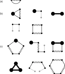
the contributions to the free energy, given in Eq. (18), of the terms that arise from the cumulant expansion can be written as dia-grams. A diagram consists of two types of elements: vertices and bonds. For the systems that we consider, there are three types of

Soft

Matter

Accepted

Manuscript

(5)

vertices:

• ρ-circles: These are represented by a large black circle and

are associated with the termz¯α(R)(orρα(R)).

• K-vertex: These are represented with a wavy line with

small black circles at either end and come with a factor

−1

2Kαα′(R,R′). The small circle on one side of the line is

associated with the particle type indexα and particle con-figurationRand the other circle is associated withα′ and

R′.

• iψ¯v−1-vertex: These are represented with a dashed line,

rep-resenting the functionv−_αα1′(R,R′), with a small gray circle on one end, representingiψ¯α(R), and a small black circle on the

other end. This vertex is associated with a factor−v−1_i_ψ_¯_.

The vertices are connected to each other by two types of bonds:

• vK-bond: These are represented by a straight, thin line with

two small black circles at either end. This represents the function−vK,αα′(R,R′), where one circle is associated with a particle of typeα in configurationRand the other circle with a particle of typeα′in configurationR′.

• f-bond: These are given by a thick line with a large black

circle on either end. This is associated with the function fαα′(R,R′).

The value associated with a diagram is a product of the integral over the functions associated with the elements and a numerical prefactor that is composed of two parts. The first part of the prefactor 1/(n1!n2!n3!), where n1 is the numberρ-circles, n2 is

the numberK-bonds, andn3is the number ofiψ¯v−1-vertices in

the diagram; this is related to the number of ways of selecting these elements. The second part is a combinatorial factor equal to the number of ways that the elements can be connect to yield the same diagram, topologically.

The diagrams that contribute to the free energy at first or-der, second oror-der, and third order of the cumulant expansion are shown in Figs. 1(a), (b), and (c), respectively. As example of evaluating a diagram, the value of the first diagram in Fig. 1(c) is

−1

2 Z

dRρα(R)[vKKvKKvK]αα(R,R)

For this diagram, there is one ρ-circle and two K-vertices; in addition, there are four distinct ways to bond theK_{-vertices to}

theρ-circle. Therefore, the numerical prefactor is4/(1!2!0!) =2. Finally, recall that eachK _{vertex carries a factor of}₋1/2, and eachvK-bond carries a factor of−1.

Fig. 1 Diagrams contributing to the (a) first-order, (b) second-order, and (c) third-order term in the cumulant expansion.

In terms of diagrams, the free energy can be written exactly as

F[ρ,Σ] =Fig[ρ] +1 2

∑

_α

Z

dRρα(R)∆vK(R,R)

+

∑

α

Z

dRρα(R)iψ¯α(R)

−1

2_αα

∑

_′ Z

dRdR′iψ¯α(R)v_αα−1′(R,R′)iψ¯α′(R′)

+1

2Tr ln(1+Kv)

−sum of all allowed diagrams.

(20)

The allowed diagrams obey the following restrictions

• The diagram must consist of one or more vertices (i.e.ρ

-circle,K_{-vertex, or}v−1_i_ψ_¯_{-vertex); the diagram consisting}

of a singleρ-circle is not allowed.

• The diagram must be connected. There must be a path from

every vertex to another.

• Twoρ-circles can be connected by at most one f-bond; f

-bonds can only be incident toρ-circles (i.e., they cannot di-rectly attach to av−1iψ¯-vertex or either end ofK ₋vertex.

ρ-circles can be incident to any number ofvK-bonds.

• Theρ-circles must not be nodal; that is, the diagram must

not become disconnected if aρ-circle is removed.

Soft

Matter

Accepted

Manuscript

[image:5.612.316.566.53.335.2]

(6)

• Both ends of aK-bond must be incident to avK-bond.

• Everyv−1iψ¯-vertex must be incident to avK-bond.

Note that whenK _{is set to zero, this representation will lead to}

the Mayer cluster expansion for a simple fluid.

This expression for the Helmholtz free energy functional is for-mally exact; the difficulty in evaluating it is the contribution of the infinite number of terms that is represented by the sum over allowed diagrams. In the following, we will discuss methods to approximate this term. The first method is the cumulant expan-sion, and the second is a summation of subsets of diagrams.

The cumulant expansions typically used in the field theory of electrolytes are typically truncated at first or second order, such as that presented in the previous section. Thenth order cumulant term only has diagrams composed ofn vertices. Only a finite set of diagrams are included at a given order of the expansion, and the contribution of all other diagrams are neglected. We can obtain a higher order approximation by summing over an infinite set of diagrams. In particular, we can exactly sum over all linear and ring diagrams (diagrams with at most one loop). We will consider this in later sections. In the following, we will discuss in more detail the issues involved in using approximate expressions for the free energy. In the next section, we begin our analysis with the first order cumulant expansion.

2.4 First order cumulant approximation

The first order cumulant approximation consists of just using the single diagram given in Fig. 1(a). The corresponding expression for the Helmholtz free energy is

F=Fig[ρ] +1 2

∑

_α

Z

+

_∑

α

Z

dRρα(R)iψ¯α(R)

−1

2_αα

∑

′

Z

dRdR′iψ¯α(R)vαα−1′(R,R′)iψ¯α′(R′)

+1

2Tr[ln(1+Kv)−KvK] +···

(21)

In order to complete the specification of the theory, we need some manner to determine the values of the arbitrary functions

¯

ψαandKαα′.. For the exact free energy, the choice ofψ¯ andK

(or equivalentlyvK) is completely arbitrary, and, consequently,

none of the physically observable properties of the system should depend on the values of these quantities. As all static equilibrium properties of the system can, in principle, be derived from the partition function, the exact partition function should be indepen-dent of the variablesψ¯ andK. This implies that the functional derivatives of the free energy with respect to these functions at all orders should vanish:

δm+n_F

δψ¯α1(r1)···δψ¯αm(rm)δKα₁′α₁′′(r′1,r′′1)···δKαn′αn′′(r′n,r′′n)

=0.

Although the exact free energy functional is independent of the choice ofψ¯ andK_{, an approximate free energy will, in general,}

have a dependence. There is then the question as to what is the optimal choice for these parameters.

One obvious criterion to determine the functions is to make the first order derivative of the free energy with respect to the func-tion equal to zero. In this case, the value of the mean interacfunc-tion potentialsψ¯α(R)are given by

δF

δiψ¯α(R)=0. (22)

For the first order cumulant approximation, this yields:

¯

ψα(R) =

∑

αα′

Z

dRvαα′(RR′)ρα′(R′). (23)

So we see thatψ¯α(R)can be identified with the interaction field

that a particle of typeα experiences in the system. The value of the screening function K _{is determined by making the free}

energy stationary:

δF

δK_αα_′_(R,R′₎=0. (24)

For the first order cumulant approximation, the screening func-tion is given by:

K_αα′(R,R′) =δαα′δd(R−R′)ρα(R). (25)

This criterion for selecting the mean field and screening func-tion has the addifunc-tional technical benefit that the first order deriva-tives of the free energy with respect to any of the properties of the system (e.g.,ραorvαα) only needs to be performed on terms

where these properties explicitly appear. That is, the implicit de-pendence ofψ¯ andK _{can be neglected.}

Interestingly, at first order, the cumulant expansion possesses a variational condition: the value of the free energy for any ar-bitrary value of ψ¯ and K will be greater than the exact value of the free energy. Consequently, it is natural to choose the val-ues of these functions such that the approximate free energy is minimized.

Imposing the stationary condition only removes the depen-dence of the approximation free energy functional onK at first order. Higher order functional derivative of the free energy will, in general, still be non-zero. The fact that for the first order cumu-lant approximation the stationary condition minimizes the system free energy relies on the second functional derivative of the free energy being positive.

For the exact free energy functional, this property should also hold for the higher order derivatives; however, it is not true for a general approximate free energy functional. Non-vanishing val-ues of the higher order derivatives will lead to inconsistencies in the theory that are related to higher order correlation functions computed through different routes. This will also lead to incon-sistencies in the evaluation of various thermodynamic properties (e.g., virial and compressibility routes of computing the pressure).

As an example, consider the total correlation functionh. This can be determined from the free energy through the relation1

δF

δvαα′(R,R′)=

1

2ρα(R)[1+hαα′(R,R ′_)]ρ

α′(R′) (26)

Soft

Matter

Accepted

Manuscript

(7)

The total correlation function for the first cumulant approxima-tion is given by

hαα′(R,R′) =−vK,αα′(R,R′). (27) This is the Debye-Hückel approximation for the total correlation function, which consists of “chains” of convolutions of the inter-actions between particles.

From the total correlation function, the direct correlation func-tion cαα′(R,R′) can be defined through the Ornstein-Zernike equation,

hαα′(R,R′) =cαα′(R,R′)

+

_∑

α′′

Z

dR′′cαα′(R,R′′)ρα′′(R′′)hαα′(R′′,R′).

With this, we find

cαα′(R,R′) =−vαα′(R,R′)

Within this approximation, the direct correlation function is just the bare interaction between particles. Note that is precisely the mean-spherical approximation, which has been used extensively to model electrolyte systems such as the primitive model, for sys-tems without a hard-core, excluded volume interaction (e.g., the ultrasolft electrolyte model26,26). This approximation yields the correct long range behavior.

The direct correlation function can also be determined from the second functional derivative of the free energy with respect to density:

δ2_F

δ ρα(R)δ ρα′(R′)=

δαα′

ρα(R)δ

d_(R

−R′)−cαα′(R,R′). (28)

This gives:

cαα′(R,R′) =v2K,αα′(R,R′)−vαα′(R,R′) +···

This expression for the direct correlation function is not consis-tent with the pair correlation function derived previously. This represents an inconsistency in the expression for the free energy functional.

The first order cumulant approximation can, in principle, be improved by including higher order terms. Unfortunately, the ac-curacy does not improve very quickly with the addition of these terms. In the next sections, we will consider adding the contribu-tion of infinite sets of diagrams.

2.5 Chain diagrams

The first infinite set of diagrams that we can exactly sum are chains. These are diagrams that consist of elements that are linked in a linear manner. Examples of diagrams in this set are shown in Fig. 2. The class of chain diagrams can be divided into three different categories, depending on the number ofρ-circles they contain. In the following, we separately describe each of these classes of diagrams and present their contributions to the free energy.

C0: The first class of chain diagrams that we consider are those with no ρ-circles. These diagrams all consist of terminal iψ¯v−1-vertices which are each directly connected to vK

-bonds, followed then by a series of alternatingK_{-bonds and}

vK-bonds. Examples of diagrams in this class are shown in

Fig. 2(C0).

The sum of all linear diagrams with noρ-circles leads to

−1

2_αα

∑

_′ Z

dRdR′iψ¯α(R)v_αα−1′(R,R′)iψ¯α′(R′).

The first term will exactly cancel the term that couplesiψ¯ to itself (see Eq. (20)), the second term cancels the coupling of the fixed charge distribution withiψ¯, and the third term is the electrostatic interaction energy of the fixed charge with itself.

C1: The next category of chain diagrams that we consider are those that contain exactly oneρ-circle. In these diagrams, theρ-circle appears on one end ot the chain and aniψ¯v−1 -vertex on the other side. These two elements are connected by an alternating series ofK_{-bonds and}_v_K_{-bonds. The first}

three of these diagrams are shown in Fig. 2(C1).

The sum of all linear diagrams with exactly one ρ-circle leads to

∑

α

Z

dRρα(R)iψ¯α(R).

The first term will cancel the term that couples the ions toiψ¯, and the second term is the electrostatic interaction energy between the mobile ions and the fixed charge.

C2: The final set of chain diagrams that we consider are those with precisely twoρ-circles. The ρ-circles appear on both ends of the diagrams and are connected to each other through a chain of alternatingvK-bonds andK-bonds.

Ex-amples of diagrams in this set are shown in Fig. 2(R2).

The sum of all linear diagrams with twoρ-circles contributes

1 2_αα

∑

′

Z

dRdR′ρα(R)Cαα′(R,R′)ρα′(R′)

where the functioncis a shifted f-bond and is given by

Cαα′(R,R′) =fαα′(R,R′) +∆vK(R,R′),

and∆vK =vK−v.

If we add the contribution of all the chain diagrams to the first cumulant approximation of the free energy, we get

F[ρ] =Fig[ρ] +1 2

∑

_α

Z

−1

2_αα

∑

_′ Z

+1

2Tr[ln(1+Kv)−KvK]− ···

Soft

Matter

Accepted

Manuscript

(8)

Fig. 2 Example of chain diagrams contributing to the free energy with (C0) noρ-circles, (C1) oneρ-circle, and (C2) twoρ-circles.

where the ellipses represent the contributions of all the allowed diagrams with one or more loops, with the exception of the dia-gram in Fig. 1(a).

Note that within this approximation, there is no dependence of the interaction fieldsψ¯α(R), so there is no need to compute

them. If we use the stationary condition to determine the screen-ing function, we get

K_αα_′_(R,_R′_{) =}_ρ_α_(R)δ_αα_′_δd_(R₋_R′₎

+ρα(R)fαα′(R,R′)ρα′(R′) +···.

(29)

Given this form for the screening function, the total correlation function (as determined by Eq. (26)) is given by

hαα′(R,R′) =fαα′(R,R′)

−

∑

α′′α′′′

Z

dR′′dR′′′(1+fρ)αα′′(R,R′′)

×vK,α′′α′′′(R′′,R′′′)(1+ρf)α′′′α′(R′′′,R′)

+···.

(30)

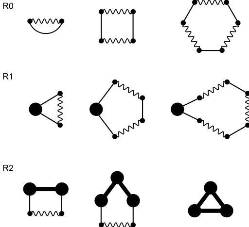
2.6 Ring diagrams

Another infinite set of diagrams that can be summed exactly are the rings, which are diagrams that consist of a single loop. Some examples of diagrams in this class are shown in Fig. 3. These dia-grams can be divided into three classes, according to the number ofρ-circles that they contain.

R0: The first class of ring diagrams that we consider are those with no ρ-circles. The simplest of these diagrams is that shown in Fig. 1(a), which is the contribution of the first or-der cumulant. All the other ring diagrams consist of alternat-ingvK-bonds andK bonds. First three of these diagrams is

Fig. 3 Example of ring diagrams contributing to the free energy with (R0) noρ-circles, (R1) oneρ-circle, and (R2) two or moreρ-circles.

shown in Fig. 3(R0). These represent the free energy of the freely fluctuating interaction fieldsψα.

The sum of all ring diagrams with noρ-circles is equal to

1

2Tr ln(1+Kv).

This term will precisely cancel the ratio of the normaliza-tion factors in the original free energy (the final term in Eq. (20)).

R1: The next class of diagrams that we consider are the ring di-agrams with exactly oneρ-circle. In these diagrams, there areρ-circle is directly connected to twovK-bonds. The

re-mainder of the diagram consists of alternatingK_{-bonds and}

vK-bonds. The first three of these diagrams are shown in

Fig. 3(R1).

The sum of all diagrams in this class contributes

1

2Trρ∆vK.

This term will exactly cancel with the self-energy terms in the free energy.

R2: The final class of diagrams are the ring diagrams with two or moreρ-circles. In these diagrams, theρ-circles must not be directly incident to aK-bond. Twoρ-circles can only be directly connected by an f-bond or by an alternating series ofvK-bonds andK-bonds. Examples of diagrams in this

class are shown in Fig. 3(R2). Note that the smallest of these diagrams is the first one shown in Fig. 3(R2).

Soft

Matter

Accepted

Manuscript

[image:8.612.39.314.48.255.2] [image:8.612.312.568.51.285.2]

(9)

The sum of all these ring diagrams gives

−1

4Tr(ρf) 2₋1

2TrρC− 1

2Tr ln(1−ρC).

Including the contribution of the chain and the ring diagrams leads to the following expression for the Helmholtz free energy functional

F[ρ] =Fig[ρ]−1

2_αα

∑

_′ Z

+1 4Tr(ρf)

2₊1

2Tr[ρC+ln(1−ρC)]

−all allowed diagrams with two or more loops,

(31)

The diagrams that appear in the final term do not depend onψ¯, so the free energy is completely independent ofψ¯.

By applying the stationary condition, the screening function is given by the solution of the integral equation

fαα′(R,R′) = [C(1−ρC)−1]αα′(R,R′) +··· (32)

where the ellipses denote contributions from functional deriva-tives of the diagrams with two or more loops. So, we see that the f-bond can be decomposed as a sum of convolutions of theC in-teractions, in the identical manner in which the total correlation function is related to the direct correlation function (i.e. through the Ornstein-Zernike equation).

By taking the functional derivative of the free energy with re-spect to the bare interaction potential (see Eq. (26)), we find that the total correlation function is given by

hαα′(R,R′) = [C(1−ρC)−1]αα′(R,R′) +···. (33)

Neglecting the contribution of diagrams with two and more loops and comparing this with the equation for the screening function, we find that thef-bond can be approximately identified with the total correlation functionh(i.e. fαα′(R,R′)≈hαα′(R,R′)), and, consequently,Ccan be identified with the direct correlation func-tion (i.e.Cαα′(R,R′)≈cαα′(R,R′)).

The definition of the f-bond, given in Eq. (13), can be written as

1+fαα′(R,R′) =e−vαα′(R,R′)+fαα′(R,R′)−Cαα′(R,R′)_. ₍₃₄₎

In approximating the total correlation function with the f-bond and the direct correlation withC, the above equation is exactly the hypernetted chain closure relation1_.

Interestingly, we have recovered hypernetted chain approxima-tion by only summing up to chain and one-loop diagrams. In the standard Mayer cluster analysis for classical fluids, the hy-pernetted chain approximation appears as the sum of diagrams with up to one loop, however, in this expansion, thef-bonds have been renormalized toh-bonds27–29. Using the stationary condi-tion with the variacondi-tional perturbacondi-tion method appears to have performed this renormalization.

3 Electrolyte systems

In this section, we examine the application of the variational per-turbation theory to electrolyte systems — specifically, multicom-ponent systems of mobile ions in the presence of a fixed charge distributionΣ(r)and dissolved in a spatially varying continuous dielectric mediumε(r). The ions can have an arbitrary internal charge distribution, such that the charge density due to an ion of typeαlocated at positionRisQα(r−R).

The electrostatic interaction energy of the system is given by

H=1 2 Z

drdr′

"

∑

k

Qα(r−Rαk) +Σ(r) #

×G0(r,r′)

"

∑

k′

Qα′(r−Rα′k′) +Σ(r′) #

−

∑

αk

eseα(Rαk)

(35)

whereRαkis the position of ion kof typeα,G0 is the Green’s

function of the Poisson equation for the system:

−_4π1 ∇_·ε(r)∇G0(r,r′) =δd(r−r′), (36)

ese_α(R)is the electrostatic self-energy of an ion of typeα

eseα(R) =

1 2 Z

drdr′Qα(R−r)Gfree(r,r′)Qα(r′−R), (37)

andGfree is the Green’s function for the Poisson equation with a

spatially uniform dielectric constant. The bare electrostatic inter-action energyvαα′(R,R′)between an ion of typeα and an ion of typeα′is

vαα′(R,R′) =

Z

drdr′Qα(R−r)Gfree(r,r′)Qα(r′−R′).

In order to simplify the presentation, we limit ourselves to the case where only electrostatic interactions are present. Non-electrostatic interactions can be included, however, this will com-plicate the vertices that appear in the diagrams. The grand parti-tion funcparti-tion for this type of system can be written as

lnZG[γ,Σ] =ln

D e−β δH[ψ]

E

0− 1 2Tr

G−₀1

G−_free1 (38)

whereh(···)i0is an average over the Hamiltonian

−βH0[ψ] =−_2β1

Z

drdr′ψ(r)G₀−1(r,r′)ψ(r′).

andδHis the Hamiltonian

−β δH[ψ] =

_∑

α

Z

dRΛ−d

α eγα(R)−

R

drQα(R−r)iψ(r)+βese

α(R)

−

Z

drΣ(r)iψ(r),

(39)

Unlike the case for the particle systems discussed in the previous section, there is only one fluctuating field, which is associated with the electrostatic potential generated by the charges in the

Soft

Matter

Accepted

Manuscript

(10)

system, both mobile and fixed. Also, the final term in the expres-sion for the grand partition function does not appear Eq. (6) for the particle system. This term captures the zero frequency disper-sion interactions in the system30,31, resulting from fluctuations in the electrostatic potential due to quantum effects. In the absence of charged particles, this leads to Lifshitz theory.

Applying the variational perturbation method, the average over the fluctuation fieldψ is is taken with respect to the Gaussian Hamiltonian

−HK =−

1 2β

Z

drdr′[ψ(r) +¯ δ ψ(r)]G_K−1(r,r′)[ψ¯(r′) +δ ψ(r′)]

where G−K1=G−

1

0 +K. The grand partition function then

be-comes

lnZG=lnhe−β δHK[δ ψ]iK −

1 2Tr ln

G−K1

G−_free1

− 1

2β Z

drdr′ψ(r)¯ G₀−1(r,r′)ψ¯(r′)−

Z

drΣ(r)iψ¯(r),

(40)

whereδHK is the Hamiltonian

−β δHK[δ ψ] =

∑

α

Z

dRΛ−_αdeγα(R)− R

drQα(R−r)[iψ¯(r)+iδ ψ(r)]+βese

α(R)

−

Z

drdr′iδ ψ(r)β−1G₀−1(r,r′)iψ(r¯ ′)

−

Z

drΣ(r)iδ ψ(r)

−1

2 Z

drdr′iδ ψ(r)K_(r,r′₎_i_{δ ψ(r}′_).

(41)

The grand partition function can be Legendre transformed to obtain the free energy functional, which is given by

F[ρ,Σ] =Fig[ρ]

+1 2

∑

_α

Z

dRdrdr′ρ(R)Qα(R−r)

×[∆GK(r,r′) +∆G0(r,r′)]Qα(r′−R)

+ Z

drQ_(r)_iψ¯(r)−_2β1

Z

drdr′iψ¯(r)G₀−1(r,r′)iψ(r¯ ′)

+1

2Tr ln(1+KG0) + 1 2Tr ln

G−₀1

G−_free1

−sum of all allowed diagrams

(42)

where∆GK =GK −G0,∆G0=G0−Gfree, andQ(r)is the total

charge density in the system, which is given by

Q(r) =

_∑

α

Z

dRρα(R)Qα(r−R) +Σ(r). (43)

The diagrams that appear in Eq. (42) are exactly the same as

those that appear in Eq. (20). The only difference is that the dot-ted lines represent(β−1_G−1

0 iψ¯−Σ)-vertices, and the thin straight

lines representGK-bonds. The f-bond is defined as in Eq. (13),

with the screened interaction potentialvK,αα′ between ions of typeαandα′given by

vK,αα′(R,R′) =

Z

drdr′Qα(R−r)βGK(r,r′)Qα′(r′−R′). (44) 3.1 Debye-Hückel theory

Taking the first order cumulant approximation to the average, which amounts to including only the single diagram in Fig. 1(a), we find

F[ρ,Σ]≈Fig[ρ]

+1 2

∑

_α

Z

dRdrdr′ρ(R)Qα(R−r)

×[∆GK(r,r′) +∆G0(r,r′)]Qα(r′−R)

+ Z

drQ_(r)_iψ(r)¯ −_2β1

Z

drdr′iψ(r)¯ G₀−1(r,r′)iψ(r¯ ′)

+1

2Tr[ln(1+KG0)−KGK] + 1 2Tr ln

G−₀1

G−_free1

(45)

where ∆GK =GK −G0. This approximation is related to the

mean spherical approximation.

The screening function can be determined through use of the stationary principle

K_(r,r′_{) =}_β

_∑

α

Z

dRQα(r−R)ρα(R)Qα(R−r′) (46)

Note that while the stationary principle ensures that the first func-tional derivative of the free energy vanishes (as required from physical considerations and the arbitrariness of the particular choice of the function), it does not guarantee that the higher or-der or-derivatives also vanish. In fact, the variational principle given by this approximation (where the optimal form of the screening function is the one which minimizes the free energy functional) is reliant on the fact that the second functional derivative of the free energy is positive.

The pair correlation function between ions is given by

hαα′(R,R′) =−

Z

drdr′Qα(R−r)βGK(r,r′)Qα′(r′−R′). (47) At sufficiently close particle distances, the pair correlation within this approximation will become negative, which is unphysical, be-tween ions with charges of the same sign. One manner to try to improve the theory is to restrict the allowed form that the screening function can sample in order to ensure that it leads to physically reasonable behavior (e.g., positive pair correlation functions).

Soft

Matter

Accepted

Manuscript

(11)

3.2 Chain diagrams

The first correction we can make is to add all the linear (chain) diagrams that contribute to the free energy to the first order cu-mulant approximation. This leads to:

F[ρ,Σ] =Fig[ρ]

+1 2

∑

_α

Z

dRdrdr′ρα(R)Qα(r−R)

×[β∆GK(r,r′) +β∆G0(r,r′)]Qα(r′−R)

+β 2 Z

drdr′Q(r)G0(r,r′)Q(r′)

−1

2

∑

_α Z

dRdR′drdr′ρα(R)Qα(r−R)

×βGK(r,r′)Qα′(r′−R′)ρα′(R′)

−1

2_αα

∑

′

Z

+1

G−₀1

G−_free1

− ···,

(48)

where the ellipses represent the contributions of the diagrams with one or more loops excluding the first cumulant.

If we use the stationary principle with the free energy, the screening function is given by

K(r,r′) =β

_∑

α

Z

dRQα(r−R)ρα(R)Qα(R−r′)

+β

∑

αα′

Z

dRdR′Qα(r−R)ρα(R)

×fαα′(R,R′)ρα′(R′)Qα′(R′−r′)

(49)

The first contribution to the screening is the same as found in the first order cumulant approximation, while the second term is due to interactions between the ions.

The total correlation function between ions is given (cf. Eq. (30)):

hαα′(R,R′) =fαα′(R,R′)

−

∑

α′′α′′′

Z

dR′′dR′′′dr′′dr′′′(1+fρ)αα′′(R,R′′)

×Qα′′(R′′−r′′)GK(r′′,r′′′)Qα′′′(r′′′−R′′′)

×(1+ρf)α′′′α′(R′′′,R′) +···.

(50)

3.2.1 Splitting theory

The standard Debye-Hückel theory works well only when the electrostatic interactions are relatively weak. In order to pro-duce an approximate free energy that would be accurate for

sys-tems also when the interactions become extremely strong, a split-ting approach was developed by Hatlo and Lue32,33. In this method, the electrostatic interactions are divided in to short-wavelengthGsand long-wavelengthGlcontributions by separat-ing the Green’s functionG0as

G0=Gs+Gl,

whereGl=P_G₀_{, and}P _{is a filter operator that depends on a}

length scaleσ that divides short wavelength phenomena (<σ) from long wavelength phenomena (>σ);σ is used as a varia-tional parameter to make the free energy stationary to first order.

The long range fluctuations associated withGl are approxi-mated using a field theoretic method (e.g., mean field theory or a variational perturbation expansion), and the interactions asso-ciated withGsare treated with a virial expansion. The resulting theory is found to be accurate for systems from the electrostatic interactions are weak all the way through to where the interac-tions are strong.

If we identifyGswithGK andGl with−∆GK, then the filter

operator is given by

P₌₁₋_G_K_G−1

0

By introducing the long range electrostatic potential ψ¯l(r) =

Pψ(r)¯ , the free energy can be written in a form that closely re-sembles the splitting theory

F[ρ,Σ] =Fig[ρ] +

_∑

α

Z

dRρα(R)βuα(R)

−1

2_αα

∑

_′ Z

+β 2 Z

drdr′Σ(r)GK(r,r′)Σ(r′)

−_2β1

Z

drdr′iψ¯l(r)Gl−1(r,r′)iψ¯l(r′) +

Z

drQ(r)iψ¯l(r)

+1

G−₀1

G−_free1 − ···, (51)

where the ellipses represent the contribution of diagrams with one or more loops excluding first cumulant, anduα(R)is a

one-body potential defined as

uα(R) =

Z

drdr′Qα(R−r)GK(r,r′)Σ(r′)

+1 2 Z

drdr′Qα(R−r)∆GK(r,r′)Qα(R−r′)

+1 2 Z

drdr′Qα(R−r)∆G0(r,r′)Qα(r′−R).

(52)

The first term in the one-body potential is the short-ranged inter-action of the ion charge with the fixed charge, the second term is related to the long-ranged self energy of the ion charge, and the final term is the image charge interaction of the ion with any

Soft

Matter

Accepted

Manuscript

(12)

dielectric inhomogeneities. This is essentially the form of the free energy given by the splitting theory at the second order cumulant expansion of the short wavelength fluctuating field. This theory has been successfully used to model the properties of systems in-teracting with the Yukawa potential34. The main exception is the presence of the next to final term in Eq. (51), which repre-sents the free fluctuations of the electrostatic potential. This term vanishes, however, if we also include the ring diagrams with no

ρ-circles (i.e. R0 diagrams).

In principle the free energy should be independent of the form selected for the filter function, however, in practice, different choices will lead to approximations with different accuracies. Us-ing the form proposed by Santangelo35,P_{= (1}₋_σ2_∇2₎_,

corre-sponds to choosing the screening function

K(r,r′) = 1

4πσ2δ

d_(r₋_r′_).

For the choice of the filter function P_{= (1}₋_σ2_∇2₊_σ4_∇4₎−1

(e.g., see Ref. 30), the corresponding expression for the screening function is

K(r,r′) = ε

4πσ2(1−σ

2_∇2₎−1_δd_(r₋_r′_).

3.2.2 Dressed ion theory

An important aspect of electrolyte systems is the long range cor-relations between charge objects. This dictates the potential of mean force between colloidal particles immersed within an elec-trolyte solution and, consequently, their aggregation behavior.

The dressed ion theory developed by Kjellander and Mitchell36 provides an exact formalism to directly analyze the long range behavior of the pair correlation function.

The direct correlation function decays exactly ascαα′(R,R′)→

−βvαα′(R−R′). We divide the direct correlation function into short-rangedcs and long-ranged contributionscl, such thatc= cs+cl, and define the short ranged direct correlation functioncs by subtracting the long-range asymptotic decay

cs,αα′(R,R′) =cαα′(R,R′)

+ Z

drdr′Qα(R−r)βG0(r,r′)Qα′(r′−R′). (53)

Similarly, we divide the total correlation function ash=hs+hl and define the short-range contribution of the total correlation functionhsthrough an Ornstein-Zernike relation

hs,αα′(R,R′) =cs,αα′(R,R′)

+

_∑

α′′

Z

dR′′cs,αα′(R,R′′)ρα′′(R′′)hs,αα′(R′′,R′).

(54)

The key result of dressed ion theory is that if the long range decay of the direct correlation function can be factorized, then the long range decay of the total correlation function also factorizes.

The long-range decay of the total correlation function is given

by a screened interaction with an effective charge.

hl,αα′(R,R′) =−

Z

drdr′Q∗α(R−r)G∗K(r,r′)Q∗α′(R′−r′), (55) whereQ∗αis the dressed charge ofαions

Q∗_α(R−r) =

_∑

α′

Z

dR′(1−csρ)−1

αα′(R,R′)Qα′(R′−r), ₍₅₆₎

G∗_K(r,r′)is a screening interaction, defined with respect to the the screening function

K∗(r,r′) =

_∑

αα′

Z

dRQα(r−R)ρα(R)Q∗α(R−r′),

through the relationG∗−K1=G−

1 0 +K∗.

If we identifyG∗K withGK, then comparing this expression

with that in Eq. (49), we find the following relationship between fandcs:

δab+fabρb= (1−csρ)−ab1.

This is just an Ornstein-Zernike relation, with f playing the role of the total correlation function, andcs playing the role of the direct correlation function. This implieshs=f.

4 One-component plasma

In order to gauge the relative accuracy of the various approxi-mations discussed in the previous section, we apply them to a one-component plasma of point charges. The charge density of the particles is given byQ(r) =qδd_(r)_{, and their charge is} neu-tralized by a uniform backgroundΣ=−ρq. The key parameter that characterizes the strength of the electrostatic interactions in the system is the coupling parameterΓ, which is defined as

Γ=

4π 3ρl

3

B 1/3

wherelB=βq2 is the Bjerrum length. For large values ofΓ, the ions are closely spaced compared to the rangelBof the Coulomb interactions, and the system is strongly coupled. For small values ofΓ, the electrostatic coupling is weak compared to the thermal motion of the ions.

4.1 Cumulant approximation

The first approximations we will consider are the first and second order cumulant expansions. At first order, the theory reduces to the Debye-Hückel approximation, where the Helmholtz free en-ergy is given by:

F V =

Fig V −

κ3

12π, (57)

with κ2₌_4πρ_lB₌₄_Γ3_/_l2

B, and κ is the inverse Debye screen-ing length. In this case, the stationary principle was used to determine the screening function, givingKˆ_{(p) =}_4πκ2_{, where}

theˆdenotes the Fourier transform of a function. The corre-sponding expression for the electrostatic interaction energy is

βU/N=√3Γ3/2_/2_{, where}_N_{is the number of ions in the system.}

Soft

Matter

Accepted

Manuscript

(13)

At second order in the cumulant expansion, the Helmholtz free energy is F V = Fig V + lB 2ρ Z p[

∆GˆK(p) +K(p)Gˆ2K(p)]

−lB

2ρ 2_ˆ

GK(0)−

1 2ρ 2_ˆ f(0) +1 2 Z p "

ln(1+Kˆ(p)_Gˆ₀_(p))

−Kˆ(p)_Gˆ_K_(p)₋1

2(Kˆ(p)GˆK(p)) 2

#

(58)

The stationary condition provides the following integral equation to be solved for the screening function:

ˆ

K_(p)_Gˆ_K_(p)Kˆ_{(p) =}_2ρ_lBKˆ_(p)_Gˆ_K_{(p) +ρ}_lB_fˆ_(p). ₍₅₉₎

The electrostatic interaction energyUis

βU N = lB 2 Z p

[∆_Gˆ_K_{(p) +}K_(p)_Gˆ2

K(p)] +

lB

2 Z

p

ˆ

GK(p)ρfˆ(p) (60)

4.2 Chain approximation

As mentioned in the previous section, including the chain dia-grams as well as the ring diadia-grams with noρ-circles leads to a theory very similar to the splitting theory. For the one-component plasma, this approximation leads to the free energy

F V ≈

Fig[ρ]

V +

lB

2ρ Z

p

∆_Gˆ_K_(p)₋lB

2ρ 2_G_ˆ

K(0)−

1 2ρ

2_f_ˆ_(0), ₍₆₁₎

The corresponding expression for the electrostatic interaction en-ergy is given by

βU N = lB 2 Z p

∆_Gˆ_K_{(p) +}lB 2 Z

p

ˆ

GK(p)ρfˆ(p). (62)

In the splitting theory, we restrict the form of the screening function to

ˆ

K_{(p) =} 1

4πσ2(1+p 2_σ2₎−1_,

whereσis used as a variational parameter.

GK(r) =

e− √ 3r 2σ r cos r 2σ+ √

3 sin r 2σ

This implies that_Gˆ_K_{(0) =}_4πσ2_and_∆_G

K(0) =−(

√

3σ)−1_{. The}

value of the parameterσis determined from the condition:

∂F

∂ σ =0. (63)

Finally, we note that adding both the chain and ring diagrams leads to the well-known hypernetted chain approximation.

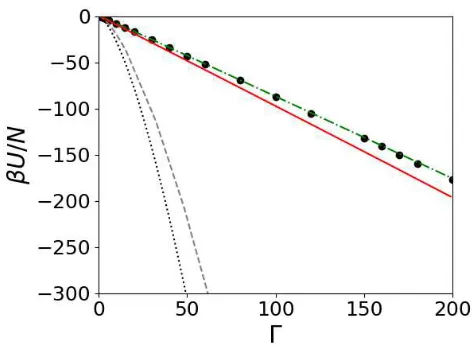
Fig. 4 Electrostatic interaction energy of a one-component plasma of point charges. The symbols are the Monte Carlo simulation data from Ref. 38, the black dotted line is the first order cumulant approximation (i.e. Debye-Hückel theory), and the black dotted line is the prediction of the second order cumulant approximation. The solid red line is the prediction of the chain + R0 approximation, and the green dashed-dotted line is the prediction of the hypernetted chain approximation.

4.3 Comparison with simulation data

In order to assess the accuracy of the various approximations, we compare their predictions with Monte Carlo37,38 and molecular dynamics simulation data for the residual electrostatic interaction energy per ion. The results are presented in Fig. 4. The symbols are the results of the simulation data.

The accuracy of the Debye-Hückel theory (black dotted line) degrades quite rapidly as the strength of the electrostatic interac-tions increases. Adding the second order correction (black dashed line) does improve the results of the theory, although not substan-tially. Both approximations severely overestimate the strength of the Coulomb interactions. This is due to the poor description of the short-wavelength fluctuations.

One method that has been used to improve the predictions of the Debye-Hückel theory is to modify the short lengthscale fea-tures of the theory by including an exclusion zone around the ions to keep the pair correlation function non-negative39,40_{or by} in-troducing a short-wavelength cutoff41–43. This approach has led to approximate theories that yield extremely good descriptions of the interaction energy.

Adding the chain and R0 diagrams (solid red line), along with restricting the form of the screening function, leads to significant improvement of the predictions. This might be expected, as this approximation is closely related to the splitting theory24. The hypernetted chain theory provides very good predictions for the interaction energy over the entire range of coupling parameters.

5 Conclusions

In this work, we have presented a diagrammatic representation of the variational perturbation method for classical particle systems interacting through pairwise additive potentials. Previously, this

Soft

Matter

Accepted

Manuscript

[image:13.612.323.559.57.232.2]

(14)

method has only been applied for low orders of the cumulant ex-pansion of the free energy functional, which leads to theories that are only accurate in the weak coupling limit. At first order in the expansion, this theory is related to the mean spherical approxi-mation. We discuss the role and choice of the screening function

K_αα′(R,R′)and consider the use of the criterion of making the free energy stationary at first order.

The diagrammatic representation of the free energy functional allow us to consider approximations involving an infinite number of terms in the cumulant expansion. In particular, we consider the corrections associated with the set of all chain diagrams and the set of all ring diagrams. We show that by including these corrections leads to the hypernetted chain approximation.

This diagrammatic approach was then applied specifically to electrolyte systems immersed in systems with a fixed background charge and (possibly) varying dielectric continuum. At first or-der, the approach reduces to the extended Debye-Hückel theory, which has been successfully to describe the influence of dielec-tric inhomogeneities on ion distribution and interactions, as well as the coupling between electrostatic and dispersion interactions. Including the chain diagrams in free energy leads to the splitting theory developed by Hatlo and Lue32,33_{, which has been very} suc-cessful in describing electrolyte systems from the weak to strong coupling limits. The link between the dressed ion theory and the splitting theory is analyzed.

The relatively simple structure of the theory is in large part due to the use of the ideal gas reference system. If another reference system is chosen, such as a hard sphere fluid, the diagrammatic structure of the theory will become more complicated. In partic-ular, there will be a variety of “particle” circles that will appear in the diagrammatic series, each corresponding to a different order direct correlation function (i.e. higher order functional deriva-tives of the free energy with respect to density). This extension will allow the application of the method to electrolyte systems that include non-electrostatic interactions.

One important factor in the variational perturbation method is the choice of the screening function. Typically, this is chosen by making the free energy functional stationary to first order. Al-though this choice provides substantial technical benefits, it does not always lead to physically reasonable results, as discussed pre-viously in the case of the pair correlation function at short dis-tances. One interesting manner that can be might be address this issue is to restrict the form that the screening function can take. This is what is done in the case of the splitting theory, when the form of the filter function is selected. This is also what is done in the hole corrected Debye-Hückel theory40for the one-component plasma, where a correlation hole is introduced in order to en-sure that the pair correlation function is positive. In the case of the variational perturbation theory, the connection between the screening function and the pair correlation will depend on the particular approximation made for the free energy functional.

Even if the stationary principle is used, the higher order func-tional derivatives of the free energy with respect to the screening function may still non-zero, which call lead to inconsistencies in the theory. This is due to the neglect of the contribution of the remaining diagrams to the free energy functional. As a result, the

value of a property will depend on the route by which it is calcu-lated (e.g., virial versus compressibility pressure). One way that this might be addressed is to add a term to the free energy func-tional that would compensate for these missing diagrams. This term could be adjusted to constrain certain higher order func-tional derivatives to zero in order to remove various inconsisten-cies which may arise.

The precise role of this term will depend on the level of ap-proximation of the free energy (i.e. the set of diagrams that are included in the approximation). In the case where the linear and ring diagrams are included, which leads to the HNC approxima-tion, the additional term will be related to the contribution of the bridge diagrams1_{, and its form will lead to different} approx-imations to the closure relation. A similar idea is taken in the development of self-consistent closure relations for integral equa-tion theories44–47. In these approaches, parameters are included in the closure relation which are then adjusted so that the certain self-consistency criteria are satisfied.

These are some of the directions we plan to pursue in future to develop an approximate theory for electrolyte systems that is ac-curate but simple enough that it can be readily applied to nonuni-form systems in complex geometries.

References

1 J.-P. Hansen and I. R. McDonald, Theory of Simple Liquids, Academic Press, 1986.

2 D. Henderson and L. Blum,J. Chem. Phys., 1978,69, 5441– 5449.

3 P. Attard, D. J. Mitchell and B. W. Ninham, J. Chem. Phys., 1988,88, 4987–4996.

4 P. Attard, D. J. Mitchell and B. W. Ninham, J. Chem. Phys., 1988,89, 4358–4367.

5 R. L. Stratonovich,Dokl. Akad. Nauk SSSR, 1957,115, 1097. 6 J. Hubbard,Phys. Rev. Lett., 1959,3, 77.

7 J. W. Negele and H. Orland,Quantum Many-Particle Systems, Addison-Wesley, Redwood City, CA, USA, 1988.

8 R. Netz and H. Orland,The European Physical Journal E, 2000, 1, 67–73.

9 R. R. Netz and H. Orland, The European Physical Journal E, 2003,11, 301–311.

10 N. V. Brilliantov,Phys. Rev. E, 1998,58, 2628–2631. 11 J.-M. Caillol,Molecular Physics, 2003,101, 1617–1634. 12 A. L. Kholodenko and A. L. Beyerlein,Phys. Rev. A, 1986,34,

3309–3324.

13 A. L. Kholodenko,J. Chem. Phys., 1989,91, 4849–4860. 14 R. D. Coalson and A. Duncan,J. Chem. Phys., 1992,97, 5653–

5661.

15 J. Ortner,Phys. Rev. E, 1999,59, 6312–6327. 16 R. R. Netz,Eur. Phys. J. E, 2001,5, 189–205.

17 D. S. Dean and R. R. Horgan,Phys. Rev. E, 2004,69, 061603. 18 D. S. Dean and R. R. Horgan,Phys. Rev. E, 2004,70, 011101. 19 H. Kleinert, Path Integrals in Quantum Mechanics, Statistics,

and Polymer Physics, World Scientific, Singapore, 2nd edn.,

1995.

Soft

Matter

Accepted

Manuscript

(15)

20 R. A. Curtis and L. Lue,J. Chem. Phys., 2005,123, 174702. 21 M. M. Hatlo, R. A. Curtis and L. Lue,J. Chem. Phys., 2008,

128, 164717.

22 S. Buyukdagli, M. Manghi and J. Palmeri, J. Chem. Phys., 2011,134, 074706.

23 L. Lue,Fluid Phase Equil., 2006,241, 236–247.

24 M. M. Hatlo, A. Karatrantos and L. Lue, Phys. Rev. E, 2009, 80, 061107.

25 J. Zinn-Justin,Quantum Field Theory and Critical Phenomena, Oxford Science, Oxford, 2002.

26 D. Coslovich, J.-P. Hansen and G. Kahl,Soft Matter, 2011,7, 1690.

27 T. Morita and K. Hiroike,Prog. Theor. Phys., 1960,23, 1003. 28 K. Hiroike,Prog. Theor. Phys., 1960,24, 317–330.

29 T. Morita and K. Hiroike,Prog. Theor. Phys., 1961,25, 537. 30 M. M. Hatlo and L. Lue,Soft Matter, 2008,4, 1582–1596. 31 R. A. Curtis and L. Lue,Curr. Opin. Colloid Interface Sci., 2015,

20, 19 – 23.

32 M. M. Hatlo and L. Lue,Soft Matter, 2009,5, 125–133. 33 M. M. Hatlo and L. Lue,Europhys. Lett., 2010,89, 25002. 34 M. M. Hatlo, P. Banerjee, J. Forsman and L. Lue, J. Chem.

Phys., 2012,137, 064115.

35 C. D. Santangelo,Phys. Rev. E, 2006,73, 041512.

36 R. Kjellander and D. J. Mitchell,J. Chem. Phys., 1994,101, 603–626.

37 S. G. Brush, H. L. Sahlin and E. Teller,J. Chem. Phys., 1966, 45, 2102.

38 W. L. Slattery, G. D. Doolen and H. E. DeWitt, Phys. Rev. A, 1982,26, 2255–2258.

39 M. J. Gillan,Journal of Physics C: Solid State Physics, 1974,7, L1.

40 N. S.,Chem Phys Lett, 1984,105, 302–307.

41 B. N. V.,Contributions to Plasma Physics, 1998,38, 489–499. 42 A. G. Moreira and R. R. Netz,Eur. Phys. J. D, 2000,8, 145–

149.

43 N. V. Brilliantov, V. V. Malinin and R. R. Netz,Eur. Phys. J. D, 2002,18, 339–345.

44 G. A. Martynov and G. N. Sarkisov, Mol. Phys., 1983, 49, 1495–1504.

45 F. J. Rogers and D. A. Young, Phys. Rev. A, 1984, 30, 999– 1007.

46 P. Ballone, G. Pastore, G. Galli and D. Gazzillo, Mol. Phys., 1986,59, 275–290.