Novel classification algorithm for ballistic target based on HRRP frame

Novel Classification Algorithm for Ballistic Target

based on HRRP frame

A.R. Persico, Student Member, IEEE and C.V. Ilioudis, Student Member, IEEE and C. Clemente, Member, IEEE, and J. J. Soraghan, Senior Member, IEEE

Abstract—Nowadays the identification of ballistic missile warheads in a cloud of decoys and debris is essential for defence systems in order to optimize the use of ammunition resources, avoiding to run out of all the available interceptors in vain. This paper introduces a novel solution for the classification of ballistic targets based on the computation of the inverse Radon transform of the target signatures, represented by a high resolution range profile frame acquired within an entire period of the main rotation of the target. Namely, the precession for warheads and the tumbling for decoys are taken into account. Following, the pseudo-Zernike moments of the resulting transformation are evaluated as the final feature vector for the classifier. The extracted features guarantee robustness against target’s dimensions and rotation velocity, and the initial phase of the target’s motion. The classification results on simulated data are shown for different polar-izations of the electromagnetic radar waveform and for various operational conditions, confirming the validity of the algorithm.

Keywords—Ballistic Missile Defence, High Resolution Range Profile, Inverse Radon Transform, Pseudo-Zernike Moments, Ballistic Target Classification

I. INTRODUCTION

Since the early stages of the development of InterContinental-range Ballistic Missiles (ICBMs) and Submarine-Launched Ballistic Missiles (SLBMs), many countries invest annually a significant budget into re-search and production of countermeasures in order to minimize the effectiveness of Ballistic Missile Defence (BMD) systems [1]. One of the most common practices is the use of a large number of decoys, or false targets, wich aim to confuse the defence systems. Currently, different decoy strategies are available, such as replica decoys, decoys using signature diversity and decoys using anti-simulation [2]. Specifically, the lightweight decoys are a very attractive option against exo-atmospheric defences, as the missile’s warhead size and range depend on the

A.R. Persico, C.V. Ilioudis, C. Clemente and J. J. Soraghan are with University of Strathclyde, Centre for Signal and Image Processing, EEE, 204, George Street, G1 1XW, Glasgow, UK. E-mail: [email protected], [email protected], [email protected], [email protected].

weight of the total carried payload. Hence, missiles can be equipped with a large number of lightweight decoys without affecting the maximum warhead range [1]. Long-range BM move on sub-orbital trajectories and their ranges typically depend on the altitude achieved by using one ore more boosters. The longer part of a BM flight takes place in the exo-atmosphere and it is commonly known as the mid-course phase. During this phase, the lightweight decoys are released as both the decoys and the much heavier warhead travel on similar trajectories due to the absence of atmospheric drag in the vacuum of space [3]. In addition to the inten-tional decoys, missiles also release incidental debris and deployment hardware, e.g. boosters for missile launch, which can pose an additional source of interference on radar returns. In absence of reliable target identification, the defence system has to intercept all the detected targets, including decoys, in order to prevent the warhead from reaching its aim. Since the anti-ballistic missile systems have a limited number of interceptors, the chal-lenge of Ballistic Targets (BTs) classification, identifying the warhead into a cloud of decoys and debris, is of fundamental importance. Specifically, the development of classification algorithms with high level of efficiency, low computational cost and short time decision is desirable not only for ground-based and sea-based defence station, but even for the On-Board Computer carried by the interceptor. The main reason for such a need is that the defence system may have to launch its interceptors before the lightweight decoys could be discriminated in order to intercept threats very far away from the interceptor deployment site [1]. Moreover, once the warhead has been identified, it is essential for the seeker on the interceptor to determine the aim point on the Re-enter Vehicle (RV) for terminal guidance and effective impact during engagement [4].

its relatively long duration and the absence of tactical manoeuvring of targets as they are in free-flight motion. The capability to distinguish between warheads and decoys during the mid-course phase is a topic widely investigated in the literature with the developed target identification algorithms being mainly based on the dif-ferent micro-motions exhibited by BTs. Specifically, the warheads are typically spin-stabilized to ensure that they do not deviate from the intended ballistic trajectories, while also exhibiting precession and nutation motion as effect of the Earth’s gravity [4]. By contrast, decoys tumble when released by the missiles due to the gravity and the absence of a spinning motor [5], [6].

Information regarding target’s micro-motions can be ex-tracted from both Doppler and range analysis of the radar returns. The effect in the Doppler domain has been firstly described by V. Chen in [7], and it is well known as micro-Doppler effect. The authors in [3] describe an adaptive framework for BM classification, demonstrating the capability to discriminate between warheads and decoys using the micro-Doppler information. In partic-ular, this framework is based on the evaluation of the spectrogram and the Cadence Velocity Diagram (CVD), which allows to extract the cadence of the micro-Doppler frequencies within the received echo. In order to perform classification, the CVD is used as the target’s signature from which a feature vector is extracted by using several approaches, which are different in terms of computational cost and feature vector dimension. On the other hand, in range analysis the micro-motions exhibited by the target lead to range migrations of its principal scattering points which are observable through a High Resolu-tion Range Profile (HRRP) frame obtained by a wide-band radar. In particular, the use of Stepped Frequency Waveforms (SFWs) for achieving a HRRP in a BMD scenario is thoroughly discussed in [8], highlighting the distortion introduced by target’s micro-motions. In the last decades the Frequency Stepped Chirp Radars (FSCR) have found application in missile terminal guidance [9]. The authors in [9] proposed a novel algorithm for the velocity estimation for missile-borne FSCR, with the aim

and a Time-Frequency Distribution (TFD).

second approach is based on the IRT computation of the TFD of the received echo. The authors in [15] describe a new approach for cleaning the ISAR image of a target from its rotating parts by applying the IRT on a frame of target range-profiles. The rotation period is firstly es-timated, then from the IRT of the range profile frame the contribution of rotating parts is detected and filtered out. In [16] a novel technique for the extraction of precession parameters of a conical target is presented. In particular, the proposed algorithm is based on the Doppler analysis of the radar echo: the precession parameter (angle and rate) are estimated by analysing the spread of echo spectrum and the echo autocorrelation. Finally a 2-D image of target is reconstructed by applying the IRT on the echo TFD.

In this paper the results and findings on an Automatic Target Recognition (ATR) algorithm proposed in [17] are presented, with the aim to classify targets in a BMD scenario from a sequence of HRRPs. The algorithm is based on the IRT of the HRRP frame, which leads to a 2-D target signature containing information on target mo-tions and the space distribution of its principal scattering points. Then from the target’s signature a feature vector is extracted, whose elements are the pseudo-Zernike (pZ) moments extracted from the 2-D target signature. The pZ moments are very attractive for image classification due to their useful properties, such as scale, translation and rotation invariance [18]. For this specific classification approach the rotation invariance is fundamental to en-sure robustness with respect to the initial phase of the target micro-motion. In this paper, the work presented in [17] is extended by introducing additional models for the radar return, investigating the effect of the micro-Doppler modulation and different acquisition scenario such as polarization diversity. Moreover, the algorithm is tested in the case of partial data frame available for the extraction of the target’s signature.

The remainder of the paper is organized as follows. Sec-tion II introduces the target model for BM warheads and decoys. Section III describes the classification framework proposed in [17], highlighting in details how the micro-Doppler effect due to target micro-motion affects the target signature. In Section IV the effectiveness of the proposed algorithm is demonstrated and the performance analysis obtained from simulated data is shown. Section V shows the performance analysis of the framework when partial data are used for extracting the target signature. Section VI concludes the paper. The appendix contains the mathematical expressions of complex scat-tering coefficients for the considered target model.

II. RADAR HIGHRESOLUTIONRANGEPROFILE FROMBTS

In radar surveillance applications the SFWs are gen-erally used in order to achieve the HRRP of a target by increasing the system’s bandwidth. In this section the signal model for rotationally symmetric BTs is presented, analysing the effect of different target micro-motions on a HRRP frame.

A. SFWs Radar based HRRP

The SFWs comprises a sequence of N narrowband sub-pulses, known as burst, which are integrated coher-ently into a single wideband signal. The carrier frequency of each sub-pulse increases pulse by pulse.

Let us consider the transmission ofM bursts with a fixed Pulse Repetition Frequency (PRF), the transmitted signal can be written as

stx(t) = M−1

X

m=0 N−1

X

n=0

p(t−nT −mN T)ej2πfnt ₍₁₎

where T is the Pulse Repetition Interval (PRI), fn the

carrier frequency of the n-th sub-pulse, and where

p(t) =

Aejπ∆τft

2

0< t < τ

0 otherwise (2)

with A, τ and ∆f being amplitude, time duration and bandwidth of the waveform sub-pulse, respectively. For a full-band SFW, ∆f is equal to the frequency step of the sub-carrier, such that fn = fc + n∆f, with

n = 0,· · · , N −1, and where fc is the fundamental

carrier frequency. Without loss of generality, in the following analysis a system using a full-band SFW is taken into consideration and A is set equal to 1. The received echo from a target at the radio frequency is expressed as the superimposition of the signals from each principal scattering point. After the de-chirping operation, during which the received signal is mixed with reference signal, the compensation of the Residual Video Phase (RVP) and the sideling term of the echo envelope (as explained in details in [19]), the received sample corresponding to n-th sub-pulse of m-th burst is given by:

s(n, m) = NP

X

i=1

σiejρie−j

4π

cfn∆R+w(n, m) (3)

with m= 0,· · · , M−1 and n= 0,· · · , N −1, σi and

ρi are the modulus and the phase of the electromagnetic

contribution of the i-th scattering point, and ∆R =

RM C−R0, with RM C the distance between the radar

(ε, m)-th element of the HRRP frame χ can be written as

χ(ε, m) =

1

N

N−1

X

n=0

$(n)s(n, m)ej2πnN ε

2

(4)

with ε= 1, ..., N and m = 1, ..., M, and where $(·) is the smoothing window.

B. BTs micro-motion model

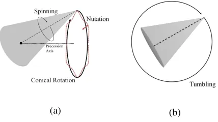
During the flight onto the exo-atmospheric part of their sub-orbits, the missile warheads exhibit precession and nutation motions as represented in Figure 1a. In partic-ular, the precession is composed by two micro-motions: the spinning of the target around its symmetry axis, and the conical movement, such that the symmetry axis rotates conically around the precession axis. The nutation is an oscillation of the symmetry axis perpendicular with respect to the precession axis. When the missile releases lightweight decoys, they starts to tumble due to the Earth gravity, as shown in Figure 1b.

(a) _(b)

Figure 1: Ballistic target micro-motions: (a) warhead; (b) decoy.

Let us consider the coordinate system ( ˆX,Y ,ˆ Zˆ) with origin in the centre of mass of the target, such that the

ˆ

Z-axis is direct along the angular velocity vector of the conical rotation (hence along the precession axis), wr,

Figure 2: Coordinate system( ˆX,Y ,ˆ Zˆ)

the direction of Line Of Sight (LOS) therefore expressed as:

n= [sin(β),0,cos(β)]T (5)

with β being the position angle with respect to the Z-ˆ axis.

It is worth noting that for a rotationally symmetric target the spinning does not change the radar view of the target. Moreover, in this paper the nutation is not taken into consideration for simplicity, since this oscillation movement does not produce significant range migration of the principal scatterers in the HRRP. Therefore, the unit vector ax, which identifies the direction of the

target’s axis of symmetry, varies on time due the conical rotation of the precession motion as follows:

c

ax(t)

=





cos(Ωrt+φ) −sin(Ωrt+φ) 0 sin(Ωrt+φ) cos(Ωrt+φ) 0

0 0 1



 



sin(θ) 0 cos(θ)





=





cos(Ωrt+φ) sin(θ) sin(Ωrt+φ) sin(θ)

cos(θ)





(6)

where Ωr = kwrk is the precession angular velocity, φ

is the initial phase of rotation and θ is the precession angle. The aspect angle α =α(t), defined as the angle between the LOS and the symmetric axis, is given by:

α(t) = cos−1(n·a_cx(t)) =

cos−1{sinβsinθcos(Ωrt+φ) + cosβcosθ}

(7)

The tumbling of decoys is defined as a rotation of the target such that the axis of symmetry is perpendicular to the rotation angular velocity vector. Hence, the aspect angle for decoys can be obtained from (7) for θ= 90◦, as follows

In the following analysis bothβandθare assumed being constant during the observation time so that the variations of the aspect angle are consequence only of the described target’s micro motions.

C. Radar Cross Section Model

According to the theory of diffraction at high fre-quency (short wavelength), the signal scattered by a target may be approximated by the sum of localized sources, represented by the principal scattering points on the object. Specifically the Radar Cross Section (RCS) of the target can be written as

σ2(f, α) =

Np

X

i=1

σi(f, α)ejρi(f,α)

2

(9)

whereNpis the total number of scatterers andσi(·)ejρi(·)

is the complex scattering coefficient of the i-th local source, which depends on both the carrier frequency f and the aspect angle α. The phase of the scattered field is [20]:

ρ(f, α) = tan−1

PNp

i=1σi(f, α) sin(ρi(f, α))

PP

i=1σi(f, α) cos(ρi(f, α))

!

(10)

The number of scattering points depends on the tar-get shape. Let us consider the local coordinate system

(ˆx,y,ˆ zˆ), defined so that the z-axis coincides with theˆ

symmetry axis of the target,cax, and the LOS belongs to the plane xˆz:ˆ

ˆ

x= ˆy×zˆ; yˆ=_cax×n; zˆ≡cax; (11)

The scattering points of the targets are located on the incident plane xˆz.ˆ

Figure 3: Local coordinate system (ˆx,y,ˆ zˆ)

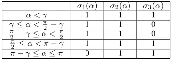
In this paper three target shapes are considered: cone, cylinder and cone plus cylinder (see Figure 4). For a conical target three principal scattering points are con-sidered: the first is in correspondence of the cone tip; the other two points are located on the intersection between

the circumference at cone bottom and the incident plane

(ˆxzˆ)(see Figure 4a). The cylindrical target is represented by four principal scattering points, two for each base, taken by intersecting the circumferences at the bases and the incident plane (see Figure 4b). Finally, for a target composed by a cone and a cylinder which share the base, five scattering points are considered. One represents the tip of the cone, while the other four are taken on the circumferences in correspondence of the cylinder bases on the incident plane (see Figure 4c).

In this work three mathematical models are considered for the complex coefficients of the target scattering points. The first is the Binary Scattering Coefficient (BSC) model, according to which the singular scattering properties of each scatterer are not taken into account for simplicity, considering the modulus of scattering coefficients as a binary function whose possible values are 0,1. Specifically, this function represents a mask which depends on the aspect angle α(t), such that its value is 1 when there is a LOS for the scattering points, and 0 otherwise.

Let us consider the possible variation ofα(t)into interval

[0, π]. For the cone, σi is 0 for the scattering point P1

(see Figure 4a) when α(t) ∈ [π−γ, π] and for P3

when α(t) ∈ [γ, π/2], with γ being the semi-angle of the cone; while for P2 the occlusion never occurs for

α(t)∈[0, π], e.g. σ2 = 1 with α(t)∈[0, π]. The values

of the coefficients modulus in different aspect angles for the cone scatterers are synthesized in Table I.

Table II shows the coefficients modulus for the cylinder scatterers for different aspect angles. Specifically,σi= 0

for P1 when α(t) = π; for P2 when α(t) = 0; for P3

when α(t)∈[0, π/2] and forP4 when α(t)∈[π/2, π].

Finally, for the cone plus cylinder, σi = 0 for P1 when

α(t) ∈ [π−γ, π]; for P2 with α(t) = π; for P3 when

α(t) = 0; for P4 when α(t) ∈ [0, π/2]; for P5 when

α(t) ∈[γ, π]. Table III synthesizes how the coefficients modulus for the cone plus cylinder vary on the aspect angle.

Table I: Modulus of the scattering coefficients for the three principal scattering points P1, P2, and P3 of the

cone, with respect to the aspect angles α.

σ1(α) σ2(α) σ3(α)

α < γ 1 1 1 γ≤α <π₂ −γ 1 1 0

π

2 −γ≤α <

π

2 1 1 0

π

2 ≤α < π−γ 1 1 1

π−γ≤α≤π 0 1 1

(a) (b) (c)

Figure 4: Target shape model: (a) Cone; (b) Cylinder; (c) Cone plus Cylinder.

Table II: Modulus of the scattering coefficients for the four principal scattering pointsP1,P2,P3 andP4 of the

cylinder, with respect to the aspect angles α.

σ1(α) σ2(α) σ3(α) σ4(α)

α= 0 1 0 0 1

0< α <π

2 1 1 0 1

α= π₂ 1 1 0 0

π

2 < α < π 1 1 1 0

α=π 0 1 1 0

Table III: Modulus of the scattering coefficients for the four principal scattering points P1,P2,P3,P4 andP5 of

the cone plus cylinder, with respect to the aspect angles α.

σ1(α) σ2(α) σ3(α) σ4(α) σ5(α)

α= 0 1 1 0 0 1

0< α < γ 1 1 1 0 1 γ≤α <π

2 1 1 1 0 0

α= π₂ 1 1 1 0 0

π

2 < α < π−γ 1 1 1 1 0

π−γ≤α < π 0 1 1 1 0

α=π 0 0 1 1 0

point projected onto the LOS. It is function of the carrier frequency of the signal, f, and of the aspect angle as follows

ρi =ρi(f, α(t))' 4πf

c [xisinα(t) +zicosα(t)] (12) where (xi, zi) are the coordinates of the i-th scattering

points onto the plane xˆz. The values of complex coeffi-ˆ

cients modulus for α(t)∈[π,2π]can be easily obtained thanks to the symmetry of the targets considered in this paper.

The other two mathematical models for the scatterer

complex coefficients refer to two different polarizations: vertical and horizontal polarization. The mathematical expressions of the coefficients are shown in the Appendix A. The phase of the complex coefficients for this two models is evaluated with respect to a reference phase centre, which can be different from the centre of mass. Since the centre of mass is stationary with respect to the micro motions, the electromagnetic field scattered by the target is generally calculated by considering the centre of mass as the phase reference centre. For this reason, (3) for both vertical and horizontal polarization RCS model is modified considering a corrective term for the phase, as follows:

s(n, m) = NP

X

i=1

σi(n, m)ejρi(n,m)e−j

4π

cfn[∆R+dM Pcos(αn,m)]

+w(n, m)

(13)

where αn,m =α(mT +nT r), σi(n, m) =σi(fn, αn,m)

and ρi(n, m) =ρi(fn, αn,m), dM P is the distance along

the symmetric axis between the centre of mass and the phase reference centre, represented respectively by the points MC and RP in Figures 4a, 4b and 4c.

such that αn,m = αm = α(mT). A SFWs radar with

a total bandwidth of 800 MHz between 2.6 and 3.4

GHz is considered, transmitting 128 sub-pulses with a PRF of 20 KHz. The range resolution guaranteed by the considered radar is 18.75 cm. For each value of aspect angle the received signal vector is zero-padded along the stepped frequency computing the IDFT over

512bins to obtain the HRRP. Moreover, a Hann window is used in order to emphasize the scatterers with lower coefficient modulus in the vertical and the horizontal polarization. Observing Figure 5b and Figure 5c it is noted that the contribution of the cone tip in the scattered field is generally lower than the contribution of the scatterers on the bottom, in both polarizations. However in a small interval of values of aspect angle (see from0◦

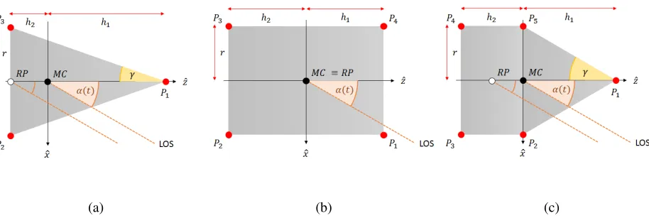
to around45◦), the tip of the cone is more visible in the vertical polarization than in the horizontal. Moreover, it is worth noting that the HRRP cannot be calculated for some values of the aspect angle with both vertical and horizontal polarization models due to the approximations considered in these RCS models (see vertical spikes in the HRRP frames shown in Figure 5b and Figure 5c). Let us consider as example the approximation for the cone which occurs for incidence nearly perpendicular to the base, specifically when α ∈ [π −αca, π], with

αca =αca(f) the axial crossover angle which varies on

the carrier frequency (see the Appendix). Figure 6 shows how the normalized RCS of the cone for α= 177◦ and the bound π −αca for the approximation vary on the

carrier frequency. It is noted that for frequencies smaller than 3 GHz the approximation occurs, while it does not for greater frequencies. This leads to a discontinuity in the RCS of simulated wide-band echo which does not allow to obtain a correct HRRP. All the details on the RCS models for both the two polarization are well described in [20].

Figure 7 shows the normalized HRRPs over 360◦, with

∆R = 0, from a cylinder whose height and diameter are 1 m and 0.7 m, respectively [17]. From Figure 7a it is noted that for each value of the aspect angle three scatterers are simultaneously visible at most. Moreover, while for the vertical polarization the scattering coef-ficients of some scatterers are higher then the others, with horizontal polarization the scattering contributions of visible scatterers are similar between each other (see Figure 7b and Figure 7c).

Figure 8 shows the normalized HRRPs over 360◦, with

∆R = 0, from a target composed by a cone plus a cylinder. The cone and cylinder heights are1.4m and0.7

m, respectively, while the diameter is 0.4 m [6]. Figure 8b and 8c show that the contribution from the cone tip is generally lower than the ones from the other scatterers.

However, even in this case the tip of the cone is more visible in the vertical polarization than in the horizontal one.

Finally it is pointed out that even for the RCS model of cylinder and cone plus cylinder for both the analysed po-larizations, some approximations are considered leading to errors in the HRRP evaluation for some values of the aspect angle, as described for the cone.

Although many models for predicting the RCS for several targets are present in the literature, it is worth noting that the scattering phenomenon depends on a large number of factors e.g. the target geometry, aspect angle and altitude with respect to radar antenna, and atmospheric factors, which lead to uncontrolled scintil-lation of the RCS. In order to take into account these fluctuation in the signal modelling, the target RCS is usually expressed as a random variable [21]. Through some experimental analysis it has been shown in [22] that the RCS of missiles shows fluctuation which can be well represented by a log-normal random variable [23]. Hence, the received signal sample s(n, m) is written as:

s(n, m) =

p

g(n, m) NP

X

i=1

σi(n, m)ejρi(n,m)

!

×

e−j4cπfn(∆R+dM Pcos[αn,m)]

+w(n, m)

(14)

where g(n, m) is a statistical sample from log-normal distribution.

III. HRRP FRAME BASEDCLASSIFICATION ALGORITHM FORBTS

In this section the classification algorithm presented in [17] which is able to extract reliable feature from the HRRP frame based on the micro-motions exhibited by BTs is described. Figure 9 represents a scheme block of the presented algorithm.

HRRP Frame Acquisition

(a) (b) (c)

Figure 5: Normalized HRRP from the cone for α ∈ [0,2π]: (a) BSC; (b) Vertical Polarization; (c) Horizontal Polarization.

Figure 6: The bound for the cone approximation for incidence nearly perpendicular to the base; the normal-ized RCS of the cone when α = 177◦ on varying the frequency.

estimated rotation rate value Ωc_r and the SFWs radar parameters. Specifically it follows:

c

M =

& c

Ωr 2πBRF

'

(15)

where BRF is the Burst Repetition Frequency, which is the number of the entire sub-pulses sequences transmitted in a second. It is worth noting that an approximation error may occur due to the fact that the number of bursts to cover an entire rotation period is not an integer.

Figure 10 represents the HRRP frame acquisition scheme, where two possible configuration are illustrated. In the first configuration (red lines in Figure 10) the estimation of the rotation rate, and consequently of the number Mc of bursts making up the HRRP frame, is computed by using primary observations of the target by cooperative system. Then the SFWs radar will transmit

c

M bursts for generating the frame for the classification

algorithm. In the second configuration (green lines in Figure 10), data acquired directly by the SFWs radar are used for the estimation of Mc. Then the selection data block will extract the sequence of bursts for the classification directly from the available data.

The received signals from each bursts are processed as described in Section II-A in order to obtain a HRRP frame from the target. The output of the first block is the matrix, χ, whose each column contains the HRRP from a single burst.

A. Signature Extraction

The signature extraction block is composed of two sub-blocks, namely the pre-processing and the IRT block, as shown in Figure 9. The pre-processing block consists of two steps. The first is the normalization of each HRRP which makes up the frame with respect to its own maximum value:

¯

χ(ε, m) = χ(ε, m) max

ε χ(ε, m)

(16)

The second step consists of resizing the normalized frame

¯

χ around the range of centre of mass, RM C, such that

the interval of considered ranges is greater than the maximum dimension of the targets of interest. Following, the target signature I is obtained normalizing byMˆ the IRT of the output of the pre-processing block, χ˜, as follows:

I = IRT{χ˜} ˆ

M (17)

(a) (b) (c)

Figure 7: Normalized HRRP from the cylinder for α ∈ [0,2π]: (a) BSC; (b) Vertical Polarization; (c) Horizontal Polarization.

(a) (b) (c)

Figure 8: Normalized HRRP from the cone plus cylinder for α ∈ [0,2π]: (a) BSC; (b) Vertical Polarization; (c) Horizontal Polarization.

Figure 9: Algorithm block scheme.

line L defined inR2, the RT of f is [10]: Rf =

Z

L

f(x, y)dl (18)

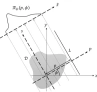
where x, y are coordinates of points on the plane, and, dl is the increment of length alongL. In order to better define the integral in (18), let us consider the definition of an arbitrary line in the normal form with respect to

the coordinate system (x, y), given by

p=xcos(φ) +ysin(φ) (19)

with φ being the inclination angle with respect to the x-axis (see Figure 11). It follows that Rf depends onp

Figure 10: HRRP frame generation block scheme.

rotating the system (x, y) by the angle φsuch that

x=pcos(φ) +ssin(φ)

y=psin(φ) +scos(φ)

the RT of f can be written as:

Rf =Rf(p, φ) =

Z ∞

−∞

f(pcos(φ) +ssin(φ), psin(φ) +scos(φ))ds

(20)

where the limits may be finite if the function f is zero outside its domain D.

Figure 11: Example of function f(x, y) domain D and a generic line L (black line) in the original (continuous lines) e rotated (dashed lines) reference coordinate sys-tem.

Let us consider the easier case in which the 2-D function is given by a delta function located at the point (x0, y0)

as follows

f(x, y) =δ(x−x0)δ(y−y0) (21)

Then its RT onto the line in (19) is

Rf(p, φ) =

Z

L

δ(x−x0)δ(y−y0)ds=

Z ∞

−∞

δ(p−p0)δ(s−s0)ds=

δ(p−x0cos(φ)−y0sin(φ))

(22)

0 0

φ0 = tan−1

x0

y0

For this reason the data obtained by the RT is known as

sinogram[27]. By contrast the IRT allows to reconstruct a 2-D function from its projections converting any sinu-soidal pattern into a point.

The space distribution function of principal target scat-terers is a 2-D function defined on the plane xˆzˆ given by the superimposition of delta functions as follows:

F = Np

X

i=1

δ(x−xi)δ(z−zi) (24)

where (xi, zi) are the coordinates of the i-th scattering

points onto the plane xˆz. In the hypothesis that theˆ

principal motion of the target is compensated, the range of each scatters Ri in the HRRP frame depends on the

aspect angle as follows:

Ri(t)

= ∆R−xisinα(t)−zicosα(t)

= ∆R−

q

x2_i +z_i2sin

α(t) + tan−1

xi

yi

(25)

Figure 12 shows the range maps and their IRT for the three scatterers of a cone considering an entire rotation period, Tr, for different couple of values of (β, θ).

The micro-motions exhibited by target leads to periodic tracks in the range-slow time domain. Specifically each scattering point generates a sinusoidal path centred at

∆R in the HRRP frame when α(t) varies into [0, π]. Then, applying the IRT, all the energy recovered from the path of a single scatterer is concentrated into a point obtaining an image which represents the profile of the object with the exact relative distances between scatterers onto planexˆzˆ(ISAR image of the object). However, from (7) it is clear that α(t) generally varies sinusoidally into

line, e.g. circumference or ellipse. For example, Figure 12e shows the IRT of the range map from a tumbling cone with (β, θ) = (60◦,90◦), where the contribution from the cone tip is concentrated in a point and the points on the base generate an ellipse, while Figure 12f shows the IRT of the range map from a precessing cone with(β, θ) = (60◦,10◦), in which each scatterer leads to a different circumference. Therefore, the IRT of HRRP frame can represent the target signature since the close lines are strictly related to the coordinates of scattering points onto the plane xˆz.ˆ

B. Feature Extraction

The pZ moments are geometrical moments with sev-eral properties, among which is that their modulus is rotational invariant. Therefore, in this work the pZ mo-ments of the target signatureI are computed in order to extract the feature vector.

Introduced in [28], the pZ moments of order o and repetition l of a 2-D image I(x, y) are calculated by projecting the image on a basis of 2-D polynomials which are defined on the unit circle as follows:

ζo,l =

o+ 1

π

2π

Z

0 1

Z

0

W_o,l∗ (ρ, θ)I(ρcosθ, ρsinθ)ρdρdθ (26)

where

Wo,l(ρ, θ) =

o−|l|

X

i=0

ρr−i(−1)i(2o+ 1−i)!

i! (o+|l|+ 1−i)! (o− |l| −i)!e jlθ

with ρ≤1.

(27)

The presented algorithm computes (O+ 1)2 pZ mo-ments, where O is the maximum order by projecting Iˆ

on the pZ polynomials, and obtaining a feature vector whose z-th element is:

Fz =|ζo,l| (28)

whereo=l= 0,· · · , O−1andz= 0,· · · ,(O+1)2−1. Since the pZ moments are defined on the unit circle, the signature I˜ is inscribed in the unit circle [18]. Finally, the feature vector given by

F = [F0F1· · ·FZ−1]. (29)

withZ = (O+ 1)2, is statistically normalised in order to avoid that polarized vector may affect the classification process. Hence, the final vector input to the classifier is:

˜

F = F −ηF

ς_F (30)

where η_F and ς_F are the statistical mean and the standard deviation of the vector F, respectively.

C. Classifier

Classifiers are mathematical techniques designed to compare the extracted features within a database, which contain the information of all the targets of interest. In this paper, the classification performances of the ex-tracted feature vectors are evaluated using the k-Nearest Neighbour (kNN) classifier. The kNN classifier is chosen as it is based on the evaluation of the Euclidean distances between the vector under test and the vectors compos-ing the traincompos-ing set of each class in order to estimate the target class. Hence, the classification performance evaluated with kNN classifier are not polarized by the properties of the classifier, and it depends only on the characteristic of features to occupy multidimensional spaces for each class sufficiently separated. However, in general other classifiers with similar characteristics could be also selected. The selection of the best classifier is outside the scope of this paper.

IV. MICRO-MOTIONVELOCITYEFFECT ONTARGET SIGNATURE

In presence of a target which moves with a radial velocity vr along the LOS, the target range varies of

about 2N vrT within the burst acquisition. The bulk

motion velocity of the target introduces a phase term, which is the major cause of distortion for the HRRP, leading to a reduced peak response and the occurrence of side-lobes. In the same way, the variation of aspect angle during the acquisition of each burst, which depends on the velocity of scatterers motion with respect to the centre of mass, represents an additional distortion factor. Let us assume that the target is tracked and the main Doppler shift due to the bulk motion is compensated perfectly, such that ∆R =RM C(t)−R0(t) = 0. From

these assumption follows that the HRRP frame shows how the distance between the radar and each principal scattering point of the target changes with time due to the micro-motions. The peak value of the range profile for each scatterer of the target locates at:

4π

c ∆fRˆi=−

4π

c ∆f Ri−

4π c

f0viT

∆f (31)

where Ri is the projection of the distance between the

i-th scatterer and the centre of mass along the LOS, and vi is the velocity of the i-th scatterer due to the

micro-motion. It is worth noting that the micro-motion of a target leads to a multi-targets (scatterers) scenario, in which each of them has a different velocity profile, given by

vi =vi(t) = (xisinα(t) −zicosα(t))

dα(t)

(a) (b) (c)

(d) (e) (f)

Figure 12: Range map and its IRT for the three points of cone considering a whole rotation period, Tr, for different

couple of values of (β, θ): (a) range map for a complete rotation of cone with (β, θ) = (90◦,90◦), (b) range map tumbling cone with (β, θ) = (60◦,90◦), (c) range map for precessing cone with (β, θ) = (60◦,10◦); (d),(e) and (f) are the IRT of the range maps (a),(b) and (c), respectively.

with

dα(t)

dt =

Ωrsin(β) sin(θ) cos(Ωrt+φ)

p

1−(sin(β) sin(θ) cos(Ωrt+φ) + cos(β) cos(θ))2

(33)

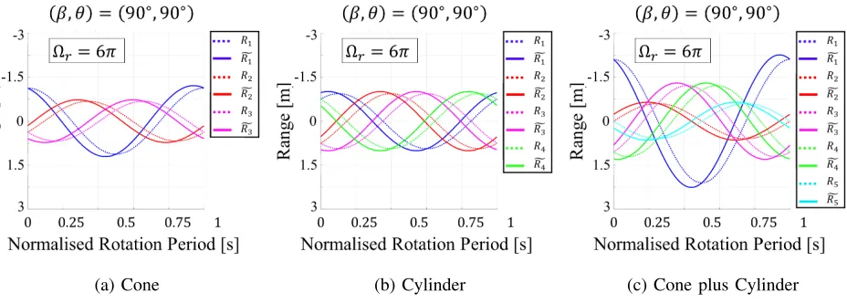
Hence, the displacement from the effective range for each scatterer is different according to its position on target surface, the target motion and the radar position. Figure 13 shows an example of how HRRP frame from the three considered shapes varies considering the stop-and-go hypothesis (dash line) and the continuous motion during the burst acquisition (continuous line). In the example shown, (β, θ) = (90◦,90◦) and

Ωr = 6π. Moreover, the occlusion and the polarization

scattering properties of the scatterers are not taken

(a) Cone (b) Cylinder (c) Cone plus Cylinder

Figure 13: Example of HRRP frame from the three considered shapes considering the stop-and-go hypothesis (dashed line) and continuous motion during the burst acquisition (continuous line), for (β, θ) = (90◦,90◦) andΩr= 6π.

The pZ moments based features guarantee robustness against rotational and scale effects on the target signature. However, in order to reduce the deforming effect due to the micro-motion and to improve the classification capabilities, the radar SFW may be adaptive to the estimated rotation rate.

V. PERFORMANCEANALYSIS

In this section the performance of the proposed clas-sification algorithm is evaluated with simulated data. The selected parameters (targets’ sizes, carrier frequency, bandwidth, etc.) have been selected in agreement to what is available in the literature [4], [6], [17], [29], [30] and on the experience of the author’s in the field being involved in research projects on the topic in the past.

The algorithm is tested considering three possible shapes for the BTs which are the cone, the cylinder and the cone plus cylinder. The cone and the cylinder have the same height and radius which are 1m and 0.375m, respectively [17]. The third shape is obtained by joining a cone whose height and radius are 1.4 m and 0.2 m, respectively, and a cylinder with a height of 0.7 m and radius 0.2m [6]. Table IV synthesizes the dimensions of the targets of interest.

Table IV: Target Dimensions.

h1[m] h2 [m] r[m]

Cone 0.750 0.250 0.375

Cylinder 0.500 0.500 0.375

Cone plus Cylinder 1.400 0.700 0.200

Six classes are considered, each of them corresponding to a particular shape and motion:

1) precessing cone; 2) tumbling cone; 3) precessing cylinder; 4) tumbling cylinder;

5) precessing cone plus cylinder; 6) tumbling cone plus cylinder;

Generally the precession angle of warheads with a con-ical shape is relatively small compared to the half cone angle [4] and its value is generally within [4◦,12◦][29]. In this work the precessing classes for each shape are obtained by fixing the precession angle θ equal to 10◦, while for the tumbling classes θ= 90◦.

Both the training and testing sets are simulated con-sidering a SFWs radar transmitting bursts composed by

128 sub-pulses with a total bandwidth of 800MHz and a PRF of 20 kHz. All the SFWs radar parameters are synthesized in Table V.

Table V: SFWs radar system parameters.

Carrier frequency [GHz] 2.600 Total bandwidth [MHz] 800 Number of sub-pulses N 128 Waveform bandwidth [MHz] 6.25 Pulse Repetition Interval [kHz] 20 Burst Repetition Interval [Hz] 156.25

The training set for each class is realized for different values of the radar position angle βu as follows

βu=u5◦ with u= 1,2,· · ·,18. (34)

the angular rotation velocities considered are

Ωrv = 2π

1 4 +

v

8

rad

s with v= 0,· · ·,22 (35)

From (15) it is pointed out that the HRRP frame length decreases as the rotation rate increases. Figure 14 shows how the number of bursts of the frame varies with the rotation rate for the SFWs radar described above. The

Figure 14: Number of bursts to obtain the HRRP frame on varying the angular rotation velocity and for the SFWs radar described in Table V

testing set for each class and for a fixed noise power and rotation rate is composed by 180samples. Each set is obtained by simulating 20 acquisitions for each value of β = 10◦ with = 1,2,· · · ,9, which are different

for the noise observation and for the initial phase of the micro-motions. The initial phase is drawn randomly from a uniform distribution [0,2π].

The performance of the proposed algorithm is evalu-ated in terms of: Probability of correct Motion identifica-tion (PM), which represents the capability to distinguish

between precessing and tumbling targets; Probability of correct Shape identification (PS), which represents the

capability to distinguish between the different shapes of targets; Probability of correct Classification (PC), the

capability to identify the motion and the actual shape of the target.

(a) (b)

Figure 15: Example of the effect of RCS logarithm fluctuation on a sequence of HRRPs from a cone for α ∈ [0,2π], simulated using the BSC model without AWGN: (a) no fluctuation; (b) RCS logarithm fluctua-tion.

three probabilities for each couple of values of SNR and rotation rate is evaluated with a Monte Carlo approach over 104 _{different runs in which 100 samples for each}

class are randomly taken from the testing dataset and classified. The k value of the k-NN classifier is chosen equal to 1.

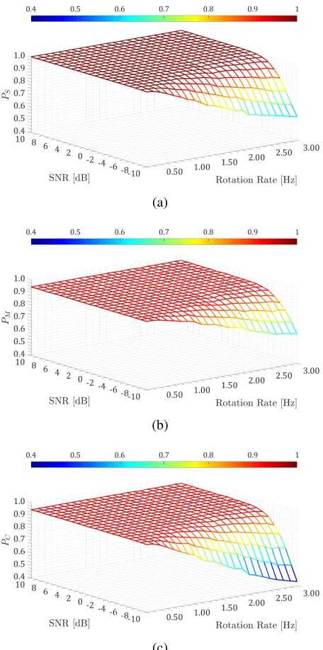
Figure 16 shows the performance obtained on varying the SNR and the angular rotation rate, considering the BSC model. In order to reduce the distortion in the HRRP due to the variation of the aspect angle within the burst interval a Hann window is used. It is observed that the performance in terms of the three probabilities increases as the SNR increases and decreases as the rotation velocity increases. The main reason is that the IRT integrates incoherently the HRRPs of the frame, increasing the SNR of the final image. The incoher-ent processing gain depends on the frame dimension: longer is the HRRP frame, higher is the processing gain. However, Figure 16a shows that PS ≥ 0.99 for SNR

greater than −5 dB for all the considered rotation rates. PC and PM are very similar for SNR greater than −5

dB since PS is close to 1. Specifically, for these SNR

values PC and PM varies within [0.93,0.95] for all the

(a)

(b)

(c)

Figure 16: Performance in terms of PS (a), PM (b) and

PC (c) by using the BSC model for the RCS.

in terms of motion recognition and correct classification are affected by the fact that the aspect angle varies in the same way when the values of the angles β and θ are switched. In this analysis there is a case in which precession and tumbling lead to the same variation of aspect angle: since the training set for each class is composed by 18 feature vectors, the ambiguity in the motion classification is around1/18≈5.5%. Hence, the maximum value reachable for PM is close to 0.95.

Figure 17 shows the performance obtained on varying SNR and angular rotation rate, considering the vertical

polarization RCS model. Similar to the previous case, Hann window is used to reduce the distortions due to the variation of the aspect angle within the burst interval and to increase the capability to observe scatterers with lower coefficients. From the results, it is observed that

(a)

(b)

(c)

Figure 17: Performance in terms of PS (a), PM (b) and

PC (c) by using the RCS model for vertical polarization.

the performance obtained with the vertical polarization model confirms the trend observed in Figure 16 for the BSC model. Figure 17a shows that PS > 0.97

for all the considered rotation rates when the SNR is greater than−5dB, reaching a maximum value of about

processing of data, especially with very low SNR values. Figure 18 shows the performance obtained on varying SNR and angular rotation rate, considering the RCS model for the horizontal polarization. Even in this case a Hann window is used to emphasize the scatterers with lower coefficients. From Figure 18a it is observed that the capability to discriminate between the different target shapes decreases lightly by using horizontal polarization rather than the vertical polarization. The main reason is due the scattering properties of points in proximity of the sharpest parts of the object. In particular, the tips of the cone and the cone plus cylinder are more visible using the vertical polarization rather than the horizontal, in agreement with the mathematical model in [20]. However, PS varies within[0.94,0.96]when the

SNR is greater than −2 dB, for all the considered values of the rotation rate. The performance in terms of PM

are similar for both the polarization models (observing Figure 17b and Figure 18b), varying within [0.92,0.95]

for all the considered rotation rates when the SNR is greater than−5dB. The loss in the performance in terms of PS using horizontal polarization leads to a loss in

PC, which varied within [0.875,0.905] when the SNR

is greater than −3 dB. Finally, it is pointed out that using the RCS model for horizontal polarization results to better performance than the ones using the BSC model for lower values of SNR and higher rotation rates. The rotation rates of precession and tumbling are gener-ally different. In fact while the warhead spinning and the decoy tumbling frequency may be similar, the precession frequency is typically an order of magnitude smaller with respect to the spinning [4]. Therefore, the system capa-bility in terms of motion recognition may be improved considering also the estimated rotation velocity. For this reason the capability to recognize the target shape is considered the most relevant in this analysis. In fact the identification of the shape may be discriminant between warheads and decoys allowing also to understand which kind of warheads the target can be (cone plus cylinder can represent a warheads with an additional booster for manoeuvring).

(b)

(c)

Figure 18: Performance in terms of PS (a), PM (b)

and PC (c) by using the RCS model for horizontal

polarization.

Finally it is important to point out that the classification algorithm is independent on initial phase of micro-motion and robust with respect to the receiver noise, the RCS scintillation and the approximation error on the HRRP frame dimension.

A. Random Burst Repetition Frequency

distribution with partial data available. In fact, using the IRT as a back-projection method, it is necessary to know the angular step computed by the target between two sequentially acquisitions. For this reason, once the rotation rate of the target is estimated and, knowing the transmission time instants of each burst, it is possible to apply the algorithm proposed in the Section III, by using a subset of HRRPs which compose the frame covering the rotation period. It is worth noting that the use of a subset of HRRPs does not require any modification in the proposed classification framework, but will only effect the set of angles in which the IRT is applied. Figure 19a shows a HRRP frame of 180 bursts con-sidering a whole rotation period of a cone obtained for (β, θ) = (90◦,90◦) considering the BSC model. Moreover, the SNR of the received signal is set equal to

10 dB. The SFW radar parameters used for simulating the acquisition are shown above, in Table V. Figure 19b emphasizes 36 bursts randomly taken from the original frame in Figure 19a, while Figure 19c and Figure 19d shows the target signatures obtained by applying the IRT on the frame in Figure 19a and Figure 19b, respectively. It is worth noting that the signature obtained from the 36

(a) (b)

(c) (d)

Figure 19: HRRP frame (a) and its IRT (b) of the three points of cone for BSC model obtained from a whole rotation period and(β, θ) = (90◦,90◦); HRRP frame (c) and its IRT (d) composed by 36 HRRPs taken randomly from the frame in (a).

bursts can properly represent the target, when the SNR on the data is sufficiently high. Nevertheless, the SNR on the final image is lower with respect to the signature obtained from the original frame, due to the incoherent integration of a smaller number of HRRPs.

This property of the algorithm is very important, since it is possible to apply the algorithm on a subset of the frame which covers the rotation period of the target, avoiding to use HRRPs affected by high level of noise or interference (e.g. jamming); on the other hand, it is possible to cre-ate simultaneously partial frames from different targets, jumping randomly from a target to another during the radar acquisitions in a multi-target scenario, computing a simultaneous classification of different objects. For the analysis of target classification performance using partial data, the BSC model is taken into account. The training set for each class is the same described above. As in the previous analysis, even in this case the testing set in this analysis is realized considering noisy observations and continuously moving targets, with the SNR of data before the signature extraction processing varying within 0 and 10 dB, and the rotation rate varying within[0.25,3]

Hz. Moreover, the RCS oscillations are represented by a lognormal distribution with unit mean and variance equal to 0.4.

Figure 20 shows the performance in terms of PS, PM

and PC, when 50% of the possible bursts are used,

randomly taken from the entire HRRP frame within a rotation period of target. It is pointed out that in this case the number of bursts composing the frame varies with the rotation rate, as shown in Figure 14. Observing Figure 20a, Figure 20b and Figure 20c it is noted that the PS, PM and PC do not change by using half of the

available bursts instead of the entire frame (shown in Figure 16) when the rotation rate is smaller than 1.50 Hz. For rotation rate greater than 1.50 Hz the algorithm performance is affected by using half of the HRRP frame, as consequence of significant decrement of Mcfor faster rotating targets. Specifically, for rotation rate of 3 Hz,PS

andPM are about 0.80, whilePC is about 0.70. Finally,

it is worth noting that the performance for each value of rotation rate does not change increasing the value of SNR from 0 to 10 dB.

Figure 22 shows the performance in terms ofPS,PM and

PC, when 36 of the potential bursts are used, randomly

taken from the entire HRRP frame within a rotation period of target. In this case, the percentage of bursts used for the algorithm varies on the angular rotation velocity, as shown in Figure 21. Moreover, the signal processing gain of the proposed algorithm is constant with respect to the target rotation rate.

(b)

(c)

Figure 20: Performance in terms of PS (a), PM (b) and

PC (c) by using 50% of the possible bursts randomly

taken from the entire HRRP frame within a rotation period of target; the BSC model is used for the RCS.

PS and PM greater than 0.90 for almost all the

con-sidered rotation rate. In particular, it is pointed out that PS increases linearly with the rotation rate, going from

about 0.90 when the rotation rate is 0.25 Hz, up to about 0.95 when it is 3 Hz, while the performance does not change for the considered values of SNR. This trend is due to completely random choice of bursts to synthesize the target signature. In fact, the entire HRRP frame for slower rotation rates contains a higher number of HRRPs, each of them corresponding to a different value

with respect to the total number of available HRRPs on varying the angular rotation velocity when 36 bursts are used for the classification algorithm.

of the aspect angle. Hence, some subsets of 36 bursts picked from the original frame may be concentrated in small regions of the frame, loosing information from a wider set of angles. On the other hand, for faster rotation rates the frame dimension decreases up to 52 bursts for rotation rate of 3 Hz. Therefore, in this case it is easier that the 36 bursts cover the observation of rotation motion over better distributed angles, leading to better extraction of target signature. In the same way, from Figure 22b and Figure 22c it is observed that PM

andPC increase linearly in[0.88,0.925]and[0.80,0.86],

respectively, when the rotation rate increases from 0.25 Hz to 3 Hz.

Therefore, it is possible to use pseudo-random burst repetition intervals to reconstruct properly the target sig-nature for the presented algorithm, obtaining satisfactory classification performance. The number of bursts and the cadence with which they may be acquired depend on the rotation rate of the target, and have to be designed in order to observe the rotated target from a suitable set of angles.

VI. CONCLUSION

In this paper a novel framework for the radar clas-sification of BTs has been presented with the aim to distinguish between warheads and decoys. The presented algorithm employs the information relative to the range migrations of the principal target scatterers and the micro-motions, which are directly observable from a HRRP frame.

(a)

(b)

(c)

Figure 22: Performance in terms of PS (a), PM (b) and

PC (c) by using 36 random bursts from the entire HRRP

frame within a rotation period of target; the BSC model is used for the RCS.

The presented algorithm is based on the use of RT applied on the HRRP frame received from the target in order to extract a 2-D target signature. A feature vector for the final classification is evaluated by computing the pZ-moments from the 2-D target signature, guaranteeing classification being independent on the initial phase of the target micro-motions (no synchronization required). The effectiveness of the proposed approach is tested on simulated SFWs radar data, obtained by considering three models for the RCS of the targets of interest:

BSC model, vertical and horizontal polarization models. The dataset for testing the algorithm has been realized for different values of the micro-motion parameters (e.g rotation velocities and precession angle), radar position angle and noise power.

The results have shown that the framework allows to discriminate between warheads and decoys with a satis-factory degree of correct shape and motion classification. In particular, the use of vertical polarization guarantees better performance than the horizontal polarization in terms of capability of shape identification and, conse-quently, of target classification. The reason is due to the higher scattering properties of points in proximity of the sharpest parts of the objects (e.g. cone tip) in the vertical polarization. The features are robust with respect to the SNR, the RCS oscillation and the HRRP distortions due to micro-movements. Specifically, this algorithm performs well in noise because the IRT has a high accumulation gain to sinusoidal curves in the target signature.

Lastly, the performance of the proposed classification algorithm was also evaluated in a random BRF scenario. Such target acquisition scenarios can occur in multi-task systems where for example the radar would be able to switch between observing different targets in a pseudo-random manner. Simulation analysis showed that the algorithm is able to obtain satisfactory classification performance when the target is observed from a suitable set of angles.

The aspects of the designed radar waveform affects the target signature and the performance of the classification algorithm. In particular, the effect on the HRRP due to the target micro-motion velocity, in terms of radar range displacement from the real distance of the scattering point from the radar, depends on the number of sub-pulses used to synthesize the assigned total bandwidth and on the PRF. These parameters also have a signif-icant impact on the final SNR of the target signature. Therefore, a further research on possible adaptable SFWs based on the estimated target micro-motion velocity could be conducted in the context of cognitive radar, improving the performance in presence of faster rotating object in lower SNR scenarios. Moreover, the design of a suitable model in agreement with to the target of interest (in terms of shape and dimension) and radar system pa-rameters (e.g. polarization and bandwidth) can also lead to a model based classification algorithm guaranteeing high performance.

APPENDIX

by the symmetric axis and the LOS, as shown in Figure 4a.

Considering the cone semi-angle,γ, and the base radius, r (see Figure 4a), the modulus of scattering coefficients are expressed in (A.1), (A.2) and (A.3), where

A= sin( π n2)

n2

r

rcsc(α)

k (A.4)

with

n1 = 2− 2γ

π (A.5)

n2 =n3= 3 2 −

γ

π (A.6)

and k = 2π_λ the propagation factor, where λ is the wavelength.

The phase of the coefficients are given by

ρ1 =

π

4 −2k(h1+h2) cos(α) (A.7)

ρ2 =

π

4 −2krsin(α) (A.8)

ρ3 =−

π

4 + 2krsin(α) (A.9)

where h1 andh2 are the distance of the tip and the base

centre with respect to the centre of mass, respectively. The choice of the sign in (A.2) and (A.3) depends on the polarization, specifically, the upper sign is associated to the vertical polarization for the incident electric field, while the lower to the horizontal polarization. Then, the scattered field from a conical target can be evaluated through (9) and (10).

The expressions of coefficients for α in proximity of values 0 and π have been updated in [20] since singu-larities arise in (A.2) and (A.3). In particular in order to evaluate the total scattered field by a conical target for incidence at near tail-on, the polarization-independent contribution from (A.2) and (A.3) is substituted by

σ2ejρ1 +σ2ejρ3

pol−ind=

2√πkr2J1(2krsin(α))

(2krsin(α)) e −jπ

2

(A.10)

J0(2krsin(α)) cos

π n2

−cos 3π

n2

−J1(2krsin(α))

2jtan(α) n2 sin

3π n2

cos_nπ

2

−cos3π_n

2

2

∓J2(2krsin(α))

cos

π n2

−1

−1#

(A.12)

where Ji(·), with i = 0,1,2, is the Bessel function of

i-th order. It is worth noting that (A.10) is independent on polarization.

Cylinder

For a cylindrical target, four principal scattering points, specifically two for each base taken by intersecting the circumferences at the bases and the plane given by the symmetric axis and the LOS, as shown in Figure 4b.

Due to the object symmetry along both the two axis of the cylinder (see Figure 4b), the expressions of the scattering coefficients are written for α ∈

0,π₂. In particular, considering the axial crossover angle, αca,

and the broadside crossover angle, αcb, defined such

that [20]

2krsin(αca) = 2.44 (A.13)

2khcos(αcb) = 2.25 (A.14)

with r the base radius and h = h1 = h2 is the

distance between the base centre and the phase reference centre, the modulus of the scattering coefficients for

α ∈

αca,π₂ −αcb

are expressed in (A.15), (A.16), (A.17) and (A.18), where

B= 2 3sin(

2π

3 )

r

rcsc(α)

k (A.19)

σ1 =







sin(π n1)

4k√2π n1

q

rcsc(α) k

n

cos_nπ

1

−cos2(π−_nγ−α)

1

o−1

0

α < π−γ

π−γ ≤α≤π (A.1)

σ2 = A

n cos π n2 −cos

3π−2α n2

o−1

∓ncos

π n2

−1

o−1

0≤α≤π (A.2)

σ3 =

   A n

cos_nπ

3

−cos3π+2α_n

3

o−1

∓ncos_nπ

3

−1o −1

0

0≤α < γ∪π

2 < α≤π

γ ≤α≤ π 2

(A.3)

σ1= B

n

cos 2π₃ −cos

π+2α 3/2

o−1

∓

cos 2π₃ −1 −1

(A.15)

σ2= B

h

cos 2π₃ −cos 4α₃ −1∓

cos 2π₃ −1 −1i (A.16)

σ3= B

n

cos 2π₃ −cos

π−2α 3/2

o−1

∓

cos 2π₃ −1 −1

(A.17)

σ4= 0 (A.18)

The phase of the coefficients are given by

ρ1=

π

4 −2k[rsin(α) +hcos(α)] (A.20)

ρ2=

π

4 −2k[rsin(α)−hcos(α)] (A.21)

ρ3=−

π

4 + 2k[rsin(α)−hcos(α)] (A.22)

ρ4=−

π

4 + 2k[rsin(α) +hcos(α)] (A.23)

For α ∈ ]0, αca] the polarization-independent

contribu-tion due to diffraccontribu-tion interjeccontribu-tion between scatters P1

and P3 (see Figure 4b) is given by

σ1ejρ1+σ3ejρ3

pol−ind=

2kr2√πJ1(2krsin(α))

2krsin(α) e −jπ

2−j2khcos(α)

(A.24)

Then, in the evaluation of the scatter field, the polarization-independent contribution from (A.15) and (A.17) is substituted by (A.24). For LOS in the axial direction (α= 0) the expression of the target RCS is

σ(α= 0) = 4πa 4

λ2 (A.25)

while the phase is

ρ(α= 0) =−π

2 −2kh (A.26)

Considering the interval α ∈ _π

2 −αcb, π 2

, the polarization-independent contribution from (A.15) and

(A.16) is substituted by

σ1ejρ1+σ2ejρ2

pol−ind=

−2h

√

rksin(2krsin(α))

2krsin(α) e jπ

4−j2krsin(α)

(A.27)

In the broadside direction (α= π₂) follows σ(α= π

2) =ka(2h)

2 _(A.28)

ρ(α= π 2) =

π

4 −2kr (A.29)

The scattered field from the cylinder for the other values of α can be evaluated thanks to the symmetry proprieties of the target.

Cylinder plus cone

Considering a target composed by a cone and a cylinder which share the base (see Figure 4c) the modulus of scattering coefficients are expressed in (A.30), (A.31), (A.32), (A.33) and (A.34), where, coherently to the other target shapes, the upper sign is associated to the vertical polarization and the lower to the horizontal polarization, and where

C₁ = sin( 2π n2)

n2

r

rcsc(α)

k (A.35)

C2 = sin(2π_n

3)

n3

r

rcsc(α)

ρ1 =

4 −2k rsin(α) + h1+ 2 cos(α) (A.40)

ρ2 =

π

4 −2k

rsin(α) + h2 2 cos(α)

(A.41)

ρ3 =

π

4 −2k

rsin(α)− h2 2 cos(α)

(A.42)

ρ4 =−

π

4 + 2k

rsin(α)−h2 2 cos(α)

(A.43)

ρ5 =−

π

4 + 2k

rsin(α) +h2 2 cos(α)

(A.44)

considering that the phase reference centre is on the symmetric axis at the same distance from the cylinder bases centres.

As done for the conical target when incidence is at and near the nose-on axial aspect, even for target composed by a cone and a cylinder (A.31) and (A.33) for 0≤α≤

γ are substituted by

σ2ejρ2 +σ4ejρ4

=

2r√πsin

π n2

n2

e−j2kh2cos(α)_×

"

J0(2krsin(α))

cos π n2 −cos 2π n2 −1

−J1(2krsin(α))

2jtan(α) n2 sin

2π n2 cos π n2 −cos 2π n2 2

∓J2(2krsin(α))

cos π n2 −1

−1#

×

(A.45)

Defining the cross over aspect angle αca as

2krsin(αca) = 2.44 (A.46)

for π − αca ≤ α ≤ π, the polarization-independent

contribution from (A.32) and (A.34) is substituted by

σ3ejρ3+σ5ejρ5

pol−ind=

2√πkr2J1(2krsin(α))

(2krsin(α)) e −jπ

2+j2kh2cos(α)

(A.47)

All other contributions to the total return from the target are well behaved in this angular region [20].

ACKNOWLEDGMENT

This work was supported by the Engineering and Phys-ical Sciences Research Council (EPSRC) Grant number EP/K014307/1; and the MOD University Defence Re-search Collaboration (UDRC) in Signal Processing

REFERENCES

[1] A.M. Sessler, J.M. Cornwall, B. Dietz, S. Fetter, S. Frankel, R.L. Garwin, K. Gottfried, L. Gronlund, G.N. Lewis, T.A. Postol, and D.C. Wright, “Countermeasure: A technical evalu-ation of the operevalu-ational effectiveness of the planned us nevalu-ational missile defense system,” Tech. Rep., Union of Concerned Scientists MIT Security Studies Program, April 2000. [2] Stephen D. Weiner and Sol M. Rocklin, “Discrimination

performance requirements for ballistic missile defense,” The Lincoln Laboratory Journal, vol. 7, no. 1, pp. 63–88, 1994. [3] A. R. Persico, C. Clemente, D. Gaglione, C. V. Ilioudis, J. Cao,

L. Pallotta, A. De Maio, I. Proudler, and J. J. Soraghan, “On model, algorithms, and experiment for micro-doppler-based recognition of ballistic targets,” IEEE Transactions on Aerospace and Electronic Systems, vol. 53, no. 3, pp. 1088– 1108, June 2017.

[4] Isaac Bankman, Eric Rogala, and Richard Pavek, “Laser radar in ballistic missile defense,” Johns Hopkins APL Technical Digest, vol. 22, no. 3, pp. 379–393, 2001.

[5] H. Gao, L. Xie, S. Wen, and Y. Kuang, “Micro-doppler signature extraction from ballistic target with micro-motions,”

IEEE Transactions on Aerospace and Electronic Systems, vol. 46, no. 4, pp. 1969–1982, Oct 2010.

[6] P. Lei, K. l. Li, and Y. x. Liu, “Feature extraction and target recognition of missile targets based on micro-motion,” in Signal Processing (ICSP), 2012 IEEE 11th International Conference on, Oct 2012, vol. 3, pp. 1914–1919.

[7] V.C. Chen, F. Li, S.S. Ho, and H. Wechsler, “Micro-Doppler effect in radar: Phenomenon, model, and simulation study,”

IEEE Transactions on Aerospace and Electronic Systems, vol. 42, no. 1, pp. 2–21, Jan 2006.

[8] M.E. Clark, “High range resolution techniques for ballistic missile targets,” Tech. Rep., British Aerospace Land and Sea Systems, Newport Road, Cowes, Isle of Wight, PO3 1 8PF, United Kingdom, 1999 British Aerospace pic.

σ1=







sin(π n1)

4k√2π n1

q

rcsc(α) k

n

cos_nπ

1

−cos2(π−_nγ−α)

1

o−1

0

α < π−γ

π−γ ≤α≤π (A.30)

σ2=

   C1 n

cos 2π₃ −cos

π+2α 3/2

o−1

∓

cos 2π₃ −1 −1

0

0≤α < π

α=π (A.31)

σ3=

(

C₂h

cos 2π₃

−cos 4α₃ −1∓

cos 2π₃

−1 −1i 0

0< α≤π

α= 0 (A.32)

σ4=

   C1 n

cos 2π₃ −cos

π−2α 3/2

o−1

∓

cos 2π₃ −1 −1

0

0≤α < γ

γ ≤α≤π (A.33)

σ5=

   C₂ n

cos 2π₃

−cosπ+2α_3/2 o −1

∓

cos 2π₃

−cos 4π₃ −1

0

π

2 < α≤π 0≤α≤ π 2

(A.34)

[10] S.R. Deans, The Radon Transform and Some of Its Applica-tions, Dover Books on Mathematics Series. Dover Publications, 2007.

[11] J. C. Wood and D. T. Barry, “Radon transformation of time-frequency distributions for analysis of multicomponent signals,” IEEE Transactions on Signal Processing, vol. 42, no. 11, pp. 3166–3177, Nov 1994.

[12] S. Stankovic, I. Djurovic, and I. Pitas, “Watermarking in the space/spatial-frequency domain using two-dimensional radon-wigner distribution,” IEEE Transactions on Image Processing, vol. 10, no. 4, pp. 650–658, Apr 2001.

[13] X. Bai, F. Zhou, M. Xing, and Z. Bao, “High resolution isar imaging of targets with rotating parts,” IEEE Transactions on Aerospace and Electronic Systems, vol. 47, no. 4, pp. 2530– 2543, OCTOBER 2011.

[14] T. Thayaparan, “Separation of target rigid body and micro-doppler effects in sar/isar imaging,” Technical memorandum, drdc ottawa tm 2006-187, Defence R&D Canada, Ottawa, 2006.

[15] Y. Hua, J. Guo, and H. Zhao, “The usage of inverse-radon transformation in isar imaging,” in 2014 IEEE International Conference on Control Science and Systems Engineering, Dec 2014, pp. 167–170.

[16] Li Kangle, Jiang Weidong, Liu Yongxiang, and Li Xiang, “Feature extraction of cone with precession based on micro-doppler,” in2009 IET International Radar Conference, April 2009, pp. 1–5.

[17] A. R. Persico, C. Ilioudis, C. Clemente, and J. Soraghan, “Novel approach for ballistic targets classification from hrrp frame,” in2017 Sensor Signal Processing for Defence Confer-ence (SSPD), Dec 2017, pp. 1–5.

[18] C. Clemente, L. Pallotta, I. Proudler, A. De Maio, J.J. Sor-aghan, and A. Farina, “Pseudo-zernike-based multi-pass auto-matic target recognition from multi-channel synthetic aperture radar,” Radar, Sonar Navigation, IET, vol. 9, no. 4, pp. 457– 466, 2015.

[19] Zhang Qun, Luo Ying, and Chen Yong-an, Eds.,

Micro-Doppler Characteristics of Radar Targets, Butterworth-Heinemann, 2017.

[20] R.A. Ross, Investigation of Scattering Principles. Volume 3. Analytical Investigation, Defense Technical Information Center, 1969.

[21] A. De Maio, A. Farina, and G. Foglia, “Target fluctuation models and their application to radar performance prediction,”

IEE Proceedings - Radar, Sonar and Navigation, vol. 151, no. 5, pp. 261–269, Oct 2004.

[22] P. Swerling, “Radar probability of detection for some additional fluctuating target cases,”IEEE Transactions on Aerospace and Electronic Systems, vol. 33, no. 2, pp. 698–709, April 1997. [23] L. Liu, M. Ghogho, D. McLernon, and W. Hu, “Pseudo

maximum likelihood estimations of ballistic missile precession frequency,” in2011 IEEE International Conference on Acous-tics, Speech and Signal Processing (ICASSP), May 2011, pp. 3796–3799.

[24] L. Liu, M. Ghogho, D. McLernon, and W. Hu, “Ballistic missile precessing frequency extraction based on maximum likelihood estimation,” in 2010 18th European Signal Pro-cessing Conference, Aug 2010, pp. 1562–1566.

[25] X. Bai and Z. Bao, “High-resolution 3d imaging of precession cone-shaped targets,” IEEE Transactions on Antennas and Propagation, vol. 62, no. 8, pp. 4209–4219, Aug 2014. [26] Honghua Yan, Xiongjun Fu, Xuehui Lei, Ping Li, and Meiguo

Gao, “Parametric estimation of micro-doppler on spatial pre-cession cone,” inProceedings of 2011 IEEE CIE International Conference on Radar, Oct 2011, vol. 1, pp. 613–616. [27] G. Kert´esz, S. Sz´en´asi, and Z. V´amossy, “Application and

prop-erties of the radon transform for object image matching,” in

2017 IEEE 15th International Symposium on Applied Machine Intelligence and Informatics (SAMI), Jan 2017, pp. 000353– 000358.