The conditional value of information of SHM : what if the manager is not the owner?

The conditional Value of Information of SHM:

what if the manager is not the owner?

Daniel Tonelli*

_{, Andrea Verzobio}

_{, Denise Bolognani}

_{, Carlo Cappello}

_{, Branko Glisic}

_,

Daniele Zonta

_{, John Quigley}

a

_{University of Trento, Via Mesiano 77, 38123 Trento, Italy;}

_{Princeton University, 59 Olden St, Princeton, NJ 08544, USA;}

c

_{University of Strathclyde, 75 Montrose Street, Glasgow, G1 1XJ, United Kingdom.}

ABSTRACT

Only very recently our community has acknowledged that the benefit of Structural Health Monitoring (SHM) can be properly quantified using the concept of Value of Information (VoI). The VoI is the difference between the utilities of operating the structure with and without the monitoring system, usually referred to as preposterior utility and prior utility. In calculating the VoI, a commonly understood assumption is that all the decisions to concerning system installation and operation are taken by the same rational agent. In the real world, the individual who decides on buying a monitoring system (the owner) is often not the same individual (the manager) who will actually use it. Even if both agents are rational and exposed to the same background information, they may behave differently because of their different risk aversion. We propose a formulation to evaluate the VoI from the owner’s perspective, in the case where the manager differs from the owner with respect to their risk prioritisation. Moreover, we apply the results on a real-life case study concerning the Streicker Bridge, a pedestrian bridge on Princeton University campus, in USA. This framework aims to help the owner in quantifying the money saved by entrusting the evaluation of the state of the structure to the monitoring system, even if the manager’s behaviour toward risk is different from the owner’s own, and so are his or her management decisions. The results of the case study confirm the difference in the two ways to quantify the VoI of a monitoring system.

Keywords: Value of Information; Bayesian Inference; Expected Utility Theory; Decision-making; Bridge Management; Fiber Optic Sensors.

1.

INTRODUCTION

Although the utility of structural health monitoring (SHM) has never been questioned in our community, only very recently a few published papers [1] [2] have clarified the way that the benefit of monitoring can be properly quantified. Indeed, seen from a mere structural engineering perspective, the utility of monitoring may not be immediately evident. Wear for a minute the hat of the manager of a Department of Transportation (DoT), responsible for the safety of a bridge: would you invest your limited budget on a reinforcing work or on a monitoring system? A retrofit work will increase the bridge load-carrying capacity and therefore its safety. On the contrary, sensors don’t change the bridge capacity, nor reduce the external loads. So how can monitoring affect the safety of the bridge? The solution to this paradox goes roughly along these lines: monitoring does not provide structural capacity, rather better information on the state of a structure; based on this information, the manager can make better decisions on the management of the structure, minimizing the chances of wrong choices, and eventually increasing the safety of the bridge over its lifespan. Therefore, to appreciate the benefit of SHM, we need to account for how the structure is expected to be operated and eventually recast the monitoring problem into a formal economic decision framework.

The basis of the rational decision making is encoded in axiomatic Expected Utility Theory (EUT), first introduced by Von Neumann and Morgenstern [3] in 1944, and later developed in the form that we currently know by Raiffa and Schlaifer [4] in 1961. EUT is largely covered by a number of modern textbooks (among the many, we recommend Parmigiani [5] to the Reader of SHM who is approaching the topic for the first time).

Within the framework of EUT, the benefit of information, such as that coming from a monitoring system, is formally quantified by the so-called Value of Information (VoI). The concept of VoI is anything but new: it was first introduced by Lindley [6] in 1956, as a measure of the information provided by an experiment, and later formalized by Raiffa and Schlaifer [4] and DeGroot [7]. Since its introduction, it has been continuously applied in manifold fields, including statistics, reliability and operational research [8] [9] [10] [11]. Its first appearance in the SHM community, however, is much more recent and dates back, in our best knowledge, to a paper published in the proceedings of SPIE by Bernal et al. in 2009 [12], followed by Pozzi et al. [13], Pozzi and Der Kiureghian [14], Thöns & Faber [1], Zonta et al. [2], - a recent state of the art can be find in Thöns [15]. In the last few years, quantifying the value of SHM has known a renewed popularity thanks to the activity of the EU-funded COST action TU1402 [16].

Broadly speaking, the value of a SHM system can be simply defined as the difference between the benefit, or expected utility u*, of operating the structure with the monitoring system and the benefit, or expect utility u, of operating the structure without the system. Both u* and u are expected utilities calculated a priori, i.e. before actually receiving any information from the monitoring system. While in u we assume the knowledge of the manager is his a priori knowledge, u* is calculated assuming the decision maker has access to the monitoring information and is sometimes referred as to preposterior utility. The difference between these values measures the value of the information to the decision maker.

Typically, it is assumed that there is one decision maker for all decisions, i.e. wheter to invest in the monitoring system as well day to day operations. This individual could be for example an idealized manager of a DoT, as the fictitious character ‘Tom’ who appears in [2]. We must recognize that in the real world the process whereby a DoT makes decision over its stock is typically more complex, with more individuals involved in the decision chain. Even oversimplifying, we always have at least two different decision stages. First a decision is made on whether or not to buy and install the monitoring system on the structure; this is a problem of long-term planning and investment of financial resources. This decision is typically carried out by a high-level manager, that in this paper we will conventionally refer to as owner, whose rationale is warranty the return on investment. The second stage is to decide on the day-to-day operation on the structure which may include, maintenance, repair, retrofit or enforcing traffic limitations, once the monitoring system is installed (or after deciding not to install it), a day to day decision. Most of the time, the manager and the owner of the structure are different individuals. Even though their choices are based on the same monitoring data and costs, they usually make different decisions, due to their different risk aversions. This means that, when the owner has to choose whether to install a monitoring system, he or she should consider that the manager could take different decisions respect to the owner’s own. The aim of this work is to formalize a rational method for quantifying the Value of Information when two different actors are involved in the decision chain: the manager, who makes decisions regarding the structure, based on monitoring data; and the owner, who chooses whether to install the monitoring system or not, before having access to these data. We start explaining why and how two different individuals, both rational and provided with the same background information, can end up with different decisions. Next, we review the basis of the VoI, which illustrates a method for evaluating the VoI in SHM-based decision-problems, and revise the framework of Zonta et al. [2], to include the difference between the manager and the owner. To illustrate how this framework works we apply it to the same decision problem reported in [2]: the Streicker Bridge case study. This is a pedestrian bridge at Princeton University campus, which is equipped with a continuous monitoring system. Some concluding remarks are reported at the end of the paper.

2.

SHM-BASED DECISION

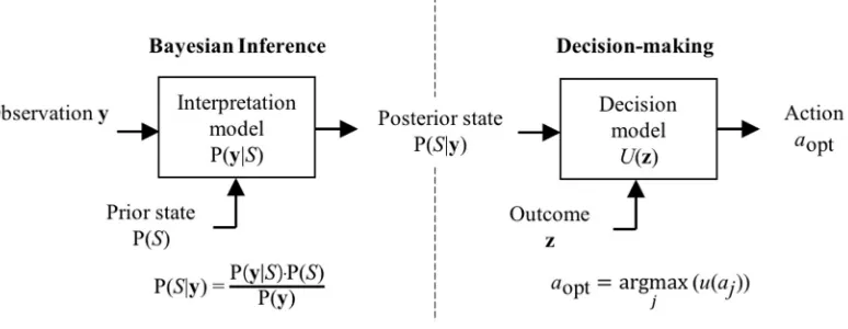
In this section, we review the concepts of Bayesian judgment, expected utility and value of information, as applied to SHM problems, following a similar path as in Cappello et al. [17] and Zonta et al. [2]. The Reader can find further examples of SHM-based decision problems in Flynn and Todd [18] [19], Flynn et al. [20] and Tonelli et al [21]. As observed in [17], SHM-based decision making (i.e., deciding based on the information from a SHM system) is properly a two-step process, which includes a judgement and a decision, as depicted in Figure 1: first, based on the information from the sensors y, we infer the state S of the structure; next, based on our knowledge of the state S we choose the optimal action aopt to take. Before proceeding with the mathematical formalization of this process let us confine the complexity of our problem through the following assumptions:

- the monitoring system provides a dataset that can be represented by a vector y;

- the structure (e.g.: one bridge) can be in a one out of N mutually exclusive and exhaustive states S1, S2, …, SN

(e.g.: S1 = ’severely damaged’, S2 = ’moderately damaged’, S3 = ’not damaged’, …);

- the decision maker can choose between a set of M alternative actions a1, a2, …, aM (for example, a1 = ‘do nothing’,

a2 = ‘limit traffic’, a3 = ‘close the bridge to traffic’, …);

- taking an action produces measurable consequences (e.g.: a monetary gain or loss, a temporary downtime of the structure, in some case causalities); the consequences of an action can be mathematically described by several parameters (e.g.: the amount of money lost, the number of day of downtime, the number of casualties), encoded in an outcome vector z;

- the outcome z of an action depends on the state of the structure, thus it is a function of both action a and state S: z(a,S); when the state is certain the consequence of an action is also deterministically known; therefore, the only uncertainty in the decision process is the state of the structure S;

- for simplicity and clarity, we refer here to the case of ‘single shot’ interrogation, which is the case when the interrogation occurs only following an event which has a single chance to happen during the lifespan; an extension to the case of multiple interrogations is also found in [2].

Figure 1. The process of SHM-based decision making.

Judgment is about understanding the state of the structure based on the observation, which is exactly what SHM is about from a logical standpoint. In the presence of uncertainty, the state of the structure after observing the sensors data y is probabilistically described by the posterior information P(S|y), and the logical inference process followed by a rational agent is mathematically encoded in Bayes’ rule [22], which reads:

P(𝑆|y) = p(𝐲|𝑆 )P(𝑆 )

p(𝐲) , (1)

where P(∙) indicates a probability and p(∙) a probability density function. Equation (1) basically says that the posterior

knowledge of the ith structural state P(Si|y) depends on the prior knowledge P(𝑆) (i.e., what I expect the state of the

structure to be before reading any monitoring data) [23] and the likelihood p(y|Si) (i.e., the probability of observing the

data given the state of the structure). Distribution p(y) is a normalization constant, referred to as evidence, calculated as:

p(𝐲) = p(𝐲|𝑆 )P(𝑆 ). (2)

Decision is about choosing the ‘best’ action based on the knowledge of the state. When the state of the system Si is

deterministically known, the rational decision-maker ranks an action based on the consequences z through a utility function

U(z). Mathematically, the utility function is a transformation that converts the vector z, which describes the outcome of an action in its entire complexity, into a scalar U, which indicates the agent’s order of subjective preference for any possible outcome.

When the state of the system is uncertain, and therefore the consequences of an action are only probabilistically known, the axioms of expected utility theory (EUT) state that the decision maker ranks their preferences based on the expected

utility u, defined as:

where ES is the expected value operator of random variable S, which we have assumed is the only uncertainty into the

problem. To prevent confusion, note that in this paper capital U indicates the utility function, while lowercase u denotes an expected utility.

Start from the case of a structure not equipped with a monitoring system, where the manager decides without accessing any SHM data. In this case the manager’s prior expected utility u(aj) of a particular action aj, depends on their prior

probabilistic knowledge P(Si) of each possible state Si:

u(aj) =∑Ni=1U z aj,Si P(Si), (4)

and consistently with EUT, the rational manager will choose that actions aopt which carries the maximum expected utility payoff u:

u=max

j u aj , aopt=argmaxj u aj . (5a,b)

In contrast, if a monitoring system is installed, and data are accessible by the agent, the monitoring observation y affects the state knowledge, and therefore indirectly their decision. This time, the posterior expected utility u(aj,y) of actions aj

depends on the posterior probabilities P(Si|y), which are now functions of the observation y:

u(𝑎, y) =∑Ni=1U z aj,Si P(Si|y) . (6)

Because the posterior probability depends on the particular observation y, in the posterior situation the expected utility is a function of y as well, and so are the maximum expected utility and the optimal choice:

u(y)=max

j u 𝑎, y , aopt=argmaxj u 𝑎, y . (7a,b)

Equation (5a) and (7a) are the utilities calculates before and after a monitoring system is interrogated. Note that, in order to evaluate the posterior utility of an action u(aj,y), we need to know the particular realization of observation y, so we

cannot evaluate the posterior utility until the monitoring system is installed and its readings are available.

How does the utility change if we have decided to install a monitoring system, but we have still to observe the sensors’ readings? Technically, what we should do is to evaluate a priori (i.e., now that the system is not installed yet) the expected value of the utility a posteriori (i.e., at the time when the system will be installed and operating). We denote this quantity

preposterior utility, u*, to separate it both from the prior and posterior utilities introduced above. The preposterior utility

u* is independent on the particular realization and can be derived from the posterior expected utility u(y) by marginalizing out the variable y, [2] [17]:

u* = E𝐲 max

j u aj,y = _Dymaxj u aj,y · p(y) dy , (8)

where distribution p(y) is the same evidence defined by Equation (2). The preposterior expected utility encodes the total expected utility of a decision process, based on the information provided by the monitoring system, but evaluated before the monitoring system is actually installed.

Finally, the Value of Information of the monitoring system is simply the difference between the expected utility with the monitoring system (preposterior utility u*) and the corresponding utility without the monitoring system (prior utility 𝑢):

VoI = u*− u = max

j u aj,y · p(y) Dy

dy−max

j u aj . (9)

In other words, the VoI is the difference between the expected maximum utility and the maximum expected utility. It is easily mathematically verified that u* is always greater or equal than u, and therefore the VoI as formulated above can only be positive. This is to say that under the assumption above SHM is always useful, consistently with the principle that “information can’t hurt” [24] as reported in Pozzi [25].

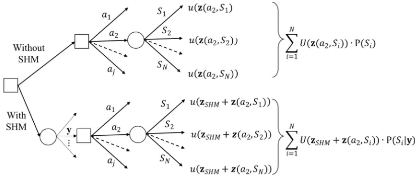
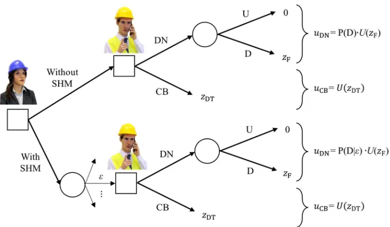
The process of deciding on the monitoring system installation can be graphically represented as a two-stage decision tree, as shown in Figure 2. At the first stage the agent decides on whether to go or not with the SHM system, while at the second stage he decides on the action a1, …, aj to undertake on the structure. The realization of the state occurs at the following

action is decided based on the information y from the monitoring system and the final outcome includes the cost zSHM of

the monitoring system. The best choice of stage one is the one that provides maximum utility, and this can be calculated by solving the two-stage tree by backward induction [5].

Figure 2. Graphical representation of the decision problem of whether or not to install a monitoring system (SHM).

3.

TWO INDIVIDUALS, TWO DECISIONS

In the classical formulation of the VoI stated above, we have implicitly assumed that the decision is taken at any stage by the same rational individual, characterized by a defined background information and utility function. We address now the problem of quantifying the VoI when two separate individuals are involved in the decision chain. We conventionally denote

manager (M) the one who makes decisions on the day-to-day operation of the structure, and owner (O), the one who is in charge of the strategic investments on the asset and decide on whether to install the monitoring system or not. Referring to Figure 2, the manager is the one who takes decisions at stage two, while the owner decides at stage one. We will refer to the classical formulation of VoI, as stated in the previous section, as to unconditional - in contrast with the conditionalVoI

which we are about to introduce.

A common misunderstanding, not only in our community, is that two individuals, if both rational and exposed to the same observation, should always end up with the same decision. In the real world, there are a number of components in the SHM-based decision process that are inherently subjective, so different decisions by different individuals should not be necessarily be seen as an inconsistency. This concept needs a deeper explanation: with reference to Figure 1, the reasons whereby two individuals, both rational, can take a different decision based on the same observation include:

- the two have a different prior knowledge of the problem – i.e. they use different priors P(S);

- they interpret differently the observation – i.e. they use different interpretation models, which are encoded in the likelihood function P(y|S);

- they have a different expectation or knowledge of the possible outcome of an action – i.e. they assume different outcome vectors z;

- they weight differently the importance of an outcome - i.e. they use different utility functions U(z).

Differences in (a) (b) and (c) are merely about background knowledge and may actually occur in the real world; however, we expect that two individuals with similar experience and education should generally agree on any of that. For example, two structural engineers with common background will probably agree on the limited importance of a bending crack visible on an unprestressed reinforced concrete beam, while a non-expert could be over-concerned. In this paper, we will assume that the two agents fully agree on (a), (b) and (c), while they only differ in the way how they weight outcomes (d), through their utility function. The utility function is not a matter of background knowledge, rather it reflects the value of the individual as to the consequence of an action.

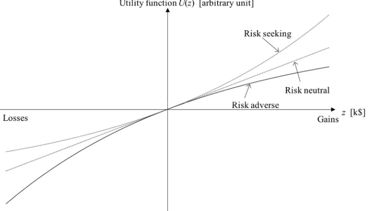
Even limiting our discussion to the case where the outcome z is just a monetary loss or gain, the utility function adopted by different people can be very different based on their particular individual risk aversion [26] [27]. For instance, an agent is risk neutral if his or her utility function U is linear with the loss or gain z, as shown in Figure 3. Since the expected utility is proportional to the probability of realization, as shown in Equation (4), risk neutrality implies indifference to a gamble with an expected value of zero. So, for example, to a risk neutral agent a 1% probability of losing $100 is equivalent to a certain loss of $1.

In practice it is commonly observed that individuals tend to reject gambles with a neutral expected payoff: in the example above individuals often prefer to pay $1 off the pocket rather than taking the risk of losing $100. This condition is referred to as risk aversion and can be graphically represented with a utility function with a concave (i.e., with negative second derivative) utility function, as shown in Figure 3. The condition of risk aversion is consistent with the observation that the marginal utility of most goods, including money, diminish with the amount of goods, or the wealth of the decision maker, as observed since Bernoulli [26].

Figure 3. Utility function for risk seeking, risk neutral and risk adverse agents.

As explained above, the risk aversion respect to a loss depends on the amount of the loss with respect to the decision maker’s own wealth or the extent of his or her own asset: when the loss is much smaller than the whole value of the asset, the agent tends to be risk neutral, while they became risk averse when the loss is a significant fraction of their asset. In our situation, the owner, who is in charge of the strategic development of the agency, typically manages a large stock of structures, and the loss corresponding to an individual structure is a much smaller than the overall asset value. In this case, it is likely that the owner is risk neutral with respect to the loss compared to the value of a single structure. In contrast the manager is responsible for the safety of a single structure: in this case the value of the structure corresponds to the value of the asset, and their behaviour is likely to be risk adverse respect to the loss of that particular structure.

To proceed with the mathematical formulation, we have to acknowledge that the two agents involved in the decision chain, the owner and the manager, may have different utility functions. We’re going to use indices (M) _or (O) _{to indicate that a}

quantity is intended from one of the other perspective. The expected utility of the manager is calculated as:

𝑢 (M)

(𝑎)= (M)𝑈 𝐳 𝑎 , 𝑆 P(𝑆 )

N

, (10)

and we may calculate the optimal action and the maximum utility from the manager perspective as in the following:

u (M)

=max

j u aj

(M)

,(M)a

opt=argmaxj u aj .

(M)

If the owner was in charge of the entire decision chain, we would end up with analogues expression of optimal action

a (O)

opt and maximum expected utility u

(O)

max, this time from the owner perspective. Observe that the optimal choice of the owner does not necessarily coincide with that of the manager, meaning that if the owner was in charge of the full decision chain they would behave differently respect to the manager. Continuing on this rationale, we can reformulate the expression of posterior utilities, preposterior utilities and VoI from the owner or the manager perspective.

However, the situation we are discussing here is different: the owner is the one who decides on the monitoring system installation, but the manager is the one who decides which is the optimal action at the second stage. Therefore, all utilities are from the owner perspective, but should be evaluated accounting for the action that the manager, not the owner, is expected to choose. In other words, the utility of the owner is conditional to the action chosen by the manager (M)a_opt. For example, the prior utility of the owner conditional to the decision expected by the manager reads:

u (O|M)

=(O)u (M)a_opt =(O)u argmax

j u aj

(M)

, (12)

where the index (O|M) _{on the utility} (O|M)_{u indicates that this utility is conditional to the manager’s choice, in opposition to}

the unconditional utility (O)u _{calculated assuming the owner in charge of the full decision chain. We can proceed}

accordingly to formulate the posterior conditional utility (the utility of the owner after the manager has observed the monitoring response):

u (O|M)

= (O)u (M)_a

opt( y) = u

(O) _argmax

j u aj,y

(M)

, (13)

and similarly the preposterior conditional utility (the utility of the owner in the expectation of what the manager would decide if a monitoring system was installed):

u* (O|M)

= (O)u argmax

j u aj,y

(M)

· p(y) dy

Dy

. ₍₁₄₎

Eventually the conditional VoI is the difference between the preposterior and the prior conditional utilities:

VoI =(O|M)u*–(O|M) u =

= (O)u argmax

j u aj,y

(M)

· p(y) dy

Dy

–(O)u argmax

j u aj

(M) (15)

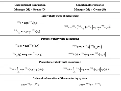
The unconditional and conditional formulations are summarized and compared in Table 1. At this point, it’s interesting to compare the unconditional and the conditional utilities, and also the value of information. The unconditional utility, prior or preposterior, is basically the owner’s utility of their favourite choice, while the conditional utility is the owner’s utility of the choice of someone else. If the two choices coincide, the conditional utility is equal to the unconditional prior utility. If they do not coincide, the manager’s choice can only be suboptimal from the owner’s perspective, and therefore the conditional utility must be equal or lower than the unconditional. Therefore, the following relationships must hold:

u (O|M)

≤(O)u , (O|M)u*_≤(O)_u*_{. (16)}

This may result in a bigger or smaller conditional VoI. In addition, contrary to the unconditional case, there is no necessity for the conditional preposterior ( | )𝑢∗ _{to be greater than the conditional posterior} ( )_𝑢∗

Table 1. Value of Information of a monitoring system in the unconditional and conditional formulation.

Unconditional formulation

Manager (M) = Owner (O)

Conditional formulation

Manager (M)

≠

Owner (O)

Prior utility without monitoring

u (O)

= max

j u aj

(O)

u (O|M)

= (O)u (M)_a

opt = u

(O) _argmax

j u aj

(M)

a (O)

opt = argmaxj u aj

(O)

Posterior utility with monitoring

u (O)

(y) =max

j u aj,y

(O)

u (O|M)

(y) = (O)u (M)_a

opt(y)

u (O|M)

(y) = (O)u argmax

j u aj,y

(M) a

(O)

opt(y) =argmaxj u aj,y

(O)

Preposterior utility with monitoring

u* (O)

= max

j u aj,y

(O)

· p(y) dy

Dy

u* (O|M)

= (O)u _argmax

j u aj,y

(M)

· p(y) dy

Dy

Value of information of the monitoring system

VoI = u(O) * – u(O) VoI =(O|M)u* – (O|M)u

4.

THE STREICKER BRIDGE CASE STUDY

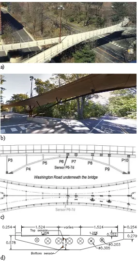
Figure 4. The Streicker bridge: view of the bridge (a)(b), location of sensors in the main span (c), main cross section (d).

a)

b)

c)

4.1 Agents

To make the case study easier to understand, we imagine the bridge managed by two agents with distinct roles:

- Susan (S) is the owner responsible for Princeton’s estate; she is Tom’s supervisor and decides on whether to install the monitoring system or not.

- Tom (T) is the manager responsible for the bridge operation and maintenance, graduated in civil engineering and registered as a professional engineer, who has to take decisions on the state of the bridge based on monitoring data, exactly as in Zonta et al. [2].

We assume that Susan and Tom are both rational individuals and that have the same knowledge background as for possible damage scenarios S of the bridge, prior information, and they have the same knowledge of the consequence of a bridge failure. They only differ in the way how to weight the seriousness of the consequences of a failure. It is probably unnecessary to remind that, while the Streicker Bridge is a real structure, the two characters, Susan and Tom, are merely fictitious and do not reflect in any instance the way how asset maintenance and operation is performed at Princeton University.

4.2 States and likelihoods

As part of this fictitious story, we suppose that both Susan and Tom are concerned by a single specific scenario: a truck, maneuvering or driving along Washington road, could collide with the steel arch supporting the concrete deck of the bridge. In this oversimplified example, we will assume that after an incident the bridge will be in one of the following two states: - No Damage (U): the structure has either no damage or some minor damage, with negligible loss of structural

capacity.

- Damage (D): the bridge is still standing but has suffered major damage; consequently, Tom estimates that there is a chance of collapse of the entire bridge.

Similar to the assumptions in [1], we assume Tom (and similarly Susan) focuses on the sensor installed at the bottom of the middle cross-section between P6 and P7 (called Sensor P6-7d, see Figure 4(c)).

We understand that for both Susan and Tom the two states represent a set of mutually exclusive and exhaustive possibilities, which is to say that P(D) + P(U) = 1. On the basis of their experience, they both agree that scenario U is more likely than scenario D, with prior pro Nobabilities P(D) = 30% and P(U) = 70%, respectively.

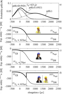
We can also assume that both use the same interpretation model, i.e. they interpret identically the data from the monitoring system. As Tom will pay attention only to the changes at the midspan sensor (labelled P6-7d in Figure 4(c)), we presume that he expects the bridge to be undamaged if the change in strain will be close to zero. However, he is also aware of the natural fluctuation of the strain, due to thermal effects, and to a certain extent due to creep and shrinkage: he estimates this fluctuation to be in the order of ±300 με. We can represent this quantity with a probability density function pdf(ε|U), with zero mean value and standard deviation σ = 300 με, which describes Tom’s expectation of the system response in the undamaged (U) state, i.e. this is the likelihood of no damage. On the other hand, if the bridge is heavily damaged (D) but still standing. Tom expects a significant change in strain; we can model the likelihood of damage pdf(ε|D) as a distribution with mean value 1000 με and standard deviation of 𝜎 = 600 με, which reflects Tom’s uncertainty of expectation.

Before the data are available, he can also predict the distribution of 𝜀, which is practically the so-called evidence in classical Bayesian theory, through the following formula:

pdf(ε) = pdf(ε|D)∙P(D) + pdf(ε|U)∙P(U) . (17)

When the measurement  is available, both update their estimation of the probability of damage consistently with Bayes’ theorem:

pdf(D|ε) = pdf(ε|D)∙P(D)

pdf(ε) , (18)

4.3 Decision model

After he assesses the state of the bridge, we assume that Tom can decide between the two following actions:

- Do nothing (DN): no special restriction is applied to the pedestrian traffic over the bridge or to road traffic under the bridge.

- Close Bridge (CB): both Streicker Bridge and Washington Road are closed to pedestrians and road traffic, respectively; access to the nearby area is restricted for the time needed for a thorough inspection, which both Susan and Tom estimates to be 1 month.

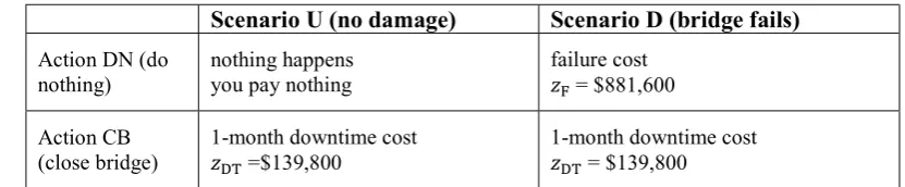
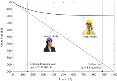
Susan and Tom agree that the costs related to each action, for each scenario, are the same as estimated in Glisic and Adriaenssens [28], and reported in Table 2.

Table 2. Costs per action and state.

Scenario U (no damage)

Scenario D (bridge fails)

nothing) nothing happens you pay nothing

failure cost

𝑧 = $881,600

Action CB

(close bridge) 1-month downtime cost 𝑧 =$139,800

1-month downtime cost

𝑧 = $139,800

However, Susan and Tom differ in their utility functions, which is the weight they apply to the possible economic losses. Susan is risk neutral, meaning that according to her a negative utility is linear with the incurred loss, as illustrated in Figure 5. Strictly speaking, a utility function is defined except for a multiplicative factor, therefore it should be expressed in an arbitrary unit sometime referred to as util [33]. Since Susan’s utility is linear with loss, for the sake of clarity we will deliberately confuse negative utility with loss, and therefore we will measure Susan’s utility in k$.

Unlike Susan, Tom is likely to behave risk adversely, i.e. his negative utility increases more than proportionally with the loss. We can describe mathematically the risk aversion classically defined in Arrow-Pratt theory [34] [35], where the level of risk aversion of an agent is encoded in the coefficient of Absolute Risk Aversion (ARA), defined as the rate of the second derivative (curvature) to the fist derivative (slope):

A(z) = U"(z)

U'(z)

.

To state Tom’s utility function, we can make the following assumptions:

- Tom’s and Susan’s reaction are virtually identical for a small amount of loss, while their way of weighting the losses departs for bigger losses.

- For small losses, therefore, the two-utility function may be confused, and we will adopt for Tom’s the same conventional unit (call it equivalent k$) for measuring utility. Tom’s utility function derivative for zero loss is equal to 1.

- We assume that Tom’s utility has constant ARA; it is easily demonstrated that a function with constant ARA and unitary derivative at zero [36] takes the form of an exponential:

U

(T) _(z)=1–e–z·θ

θ , (20)

where θ is the constant ARA coefficient: A(z) = 

- To calibrate , we assume that for a loss equal to the failure cost, Tom’s negative utility is twice that of Susan’s. This results in a constant ARA coefficient θ= -1.4249 M$-1_.

Using these assumptions, the resulting Tom’s utility function is plotted in Figure 5.

Figure 5. Representation of Susan’s and Tom’s utility functions.

4.4 Prior utility

Consider the case where Tom has no monitoring information. Based on his utility, Tom estimates the utilities involved in each action. Action CB depends only on the downtime cost zDT, while action DN depends also on his estimate of the state

of the bridge:

u (T)

DN = 𝑈

(T) _(z

F) ∙ P(D) = –528.883 k$ , (T)u_CB = (T)𝑈(zDT) = –154.940 k$ . (21)

Since the utility of action CB is clearly bigger than the utility of action DN, Tom would always choose to close the bridge after an incident if he has no better information from the monitoring system. Therefore, Tom’s maximum expected utility without the monitoring system is (T)u =(T)u_CB = -154.940 k$.

Now imagine Susan in charge of the decision: her prior utilities are different from Tom’s and their values are somewhat closer:

u (S)

DN = 𝑈

(S) _(z

F)∙P(D) = –264.480 k$ , (S)u_CB = (S)𝑈(zDT) = –139.800 k$ , (22)

but in the end, in this particular case, her optimal action would be again ‘close the bridge’. 4.5 Posterior utility

Now imagine that the monitoring system is installed and let’s go back to Tom. Since now Tom can rely on the monitoring reading, in this case the expected utility of an action is calculated using the posterior probability of damage pdf(D|ε) rather than the prior:

uCB|ε

(T) _{= u(z}

DT) , (T) uDN|ε= u(zF)∙ pdf(D|ε) (23a,b)

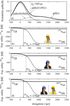
Note that since the cost of closing the bridge is independent on the bridge state, the monitoring observation  does not affect the posterior utility of closing the bridge (CB), which is always equal to -154.940 k$ as in the prior case. On the contrary, the expected utility of doing nothing (DN) does depend on the probability of having the bridge damaged, and this probability, in turn, depends on the monitoring observation through Equation (23b). Tom’s posterior expected utilities for actions DN and CB are plotted in the graph of Figure 7(b) as functions of the observation . As a rational agent, Tom will always take the decision that maximizes his utility. For very small values of , suggesting a small probability of collapse, Tom’s utility of DN is bigger than the utility of CB, and therefore Tom will keep the bridge open. Tom’s utility of closing the bridge starts exceeding the utility of doing nothing above a threshold of strain of (T)ε̅u= 170 με, and therefore Tom will always close the bridge above this threshold.

Note that this threshold is much smaller than the threshold ε̅p whereby Tom would judge the damage more likely, so there is a range of values whereby Tom, in consideration of the possible consequences, will still prefer to close the bridge even if it is more likely the bridge is not damaged. Tom’s maximum expected utility is plotted in bold in the graph of Figure 7(b).

Assume now that Susan is in charge of the decision. Since she weights the losses differently, her utility curves as functions of  are different from Tom’s, and are plotted in the graph of Figure 7(c). For the same reason, the threshold above which she would close the bridge, (S)ε̅u= 310 με, is different and much higher than Tom’s, reflecting Susan’s risk neutrality in contrast to Tom’s risk aversion. Therefore, there is a range of values of measurements, from 170  to 310 , where the two decision makers, both rational, behave differently under the same information, simply because of their different level of risk aversion.

4.6 Preposterior utility and Value of Information

Before attacking this problem, let’s first see what happens if the decision chain was in the hands of a single individual. Let us start, for example, with Tom. His preposterior utility (i.e., the prior utility of operating the bridge with the monitoring system) can be calculated with the equation:

u (T) *

= u argmax

j u(aj,ε)

(T) _{· p(ε) dε}

(T)

= – Dε

88.504 k$ , (24)

where the index (T) indicates that all the utilities are calculated from Tom’s perspective. Tom’s VoI is simply the difference between the preposterior utility and the prior utility:

VoI = (T) ∗u –(T)u = – 88.505 k$ +154.940 k$ = 66.435 k$ . (25)

Note that the VoI is a utility, not an actual amount of money, and is measured in Tom’s utility unit, which in our case is Tom’s dollar-equivalent as defined above.

Now let’s calculate the VoI from Susan’s perspective, assuming that is Susan who takes decisions at any stage of the decision chain. In this case being Susan less risk adverse than Tom, her utilities will be (S) ∗u = -84.600 k$ and (S)u* = -139.800 k$, so eventually Susan’s VoI would be:

VoI = (S) ∗u –(S)u = – 84,600 k$ + 139,800 k$ = 55.200 k$ . (26)

This practically means that, if Susan was in charge of all the decisions, she would be willing to spend up to 55.200 k$ for the information from the monitoring system.

In reality, Susan is only in charge of the purchase of the monitoring system, while the one who is going to use it is her colleague Tom. So, in taking her decision, Susan has to figure out how Tom is going to behave both with and without the monitoring system. In other words, we have to calculate the prior and preposterior utility from Susan’s perspective, but conditional to the action that Tom will undertake.

For example, to calculate the prior (without the monitoring system) conditional utility, Susan thinks: what will Tom do after an accident if no monitoring system is installed? I know Tom, and I know he will close the bridge right away (I would do the same, but that’s irrelevant). My utility, if he closes the bridge, is:

u (S|T)

= u argmax j u(aj)

(T)

(S)

= u(S)

CB = –139.800 k$ , (27)

which in this case is the same as the unconditional. And what – Susan continues to think – would Tom do if a monitoring system was installed. I know that he would look at the strain ε and he would close the bridge if ε >170  and keep the bridge open otherwise. I personally would NOT do the same, but that’s it, I have to live with Tom’s decision!

The way Susan evaluates the utility on Tom’s decisions is explained in Figure 7(d): her utilities for each possible Tom’s choice are calculated using her utility function, hence all individual curves are identical to those of Figure 7(c), However, the threshold whereby she expects the bridge is closed is Tom’s threshold, i.e. the same as in Figure 7(d). Susan’s utility of Tom’s choice is, for any value of ε:

a (S)

opt= u

( )

argmax

j u(aj,ε)

(T) _{= – 154.94 k$ , (28)}

and therefore the preposterior utility conditional to Tom is:

u (S|T) *

= u argmax

j u(aj,ε)

(T) _{· p(ε) dε}

(S)

=

Dε

–88.504 k$ (29)

Eventually, Susan’s VoI, conditional on Tom’s decision, is:

VoI (S|T)

= (S|T)u*–(S|T)u = – 88.505 k$ + 139.800 k$ = 51.295 k$ . (30)

Therefore, the conditional prior and pre-posteriors are always smaller than the corresponding unconditional: (S|T)u≤(S)u,

u*

(S|T)

≤(S)u*. In the present example, Susan and Tom agree on what to do a priori (S|T)u=(S)u, the conditional (S|T)VoI

is necessarily smaller than the conditional (S)VoI. In simple words, Susan’s rationale goes along these lines: I can exploit the monitoring system better than Tom, therefore the benefit of the monitoring system would be greater if it was me using it rather than Tom.

However, this is not the most general case. Assume for example the prior probability of damage P(D) is 10%: Susan’s prior utility of action DN (S)u_DN= -88.160 k$, small enough for Susan to keep the bridge open; on the contrary Tom’s prior utility(T)u_DN = -176.294 k$, is still big enough for Tom to close it. In this case the unconditional prior is much bigger than the conditional one, since Susan doesn’t agree with Tom’s choice, and the conditional (S|T)VoI = 103.670 k$ is much bigger than the unconditional (S)VoI= 53.217 k$, meaning that monitoring is much more useful in this case. We can almost hear Susan commenting: This Tom can’t make the right decision alone, hopefully some monitoring will help him! For sure a monitoring system is more useful to him rather than me!

5.

CONCLUDING REMARKS

The benefit of SHM can be quantified using the concept of VoI, which is the difference between the utilities of operating the structure with and without the monitoring system, commonly referred to as preposterior utility and prior utility. Being the VoI a utility, its quantification is inherently subjective and changes with the decision maker. In calculating the VoI, a commonly understood assumption is that all the decisions concerning installation of the system and operating the structure are taken by the same rational agent. In the real world, the individual who decides on buying a monitoring system (call them owner) is often not the same individual who later is going to use it (call them manager). The two, even if both rational and exposed to the same background information, may still behave differently because of their different appetites for risk. We developed a formulation to properly evaluate the VoI from the owner perspective, in the case where the manager is a different individual who differs in the way how he ranks priorities. The logic is that the owner, in evaluating the utility of the perspective monitoring system, must understand how the manager will behave downstream in response to damaging events and monitoring observations. The calculation requires the definition of the owner’s prior and preposterior utilities

conditional to the manager expected behavior.

Seen from the owner perspective, the choices of the manager are always suboptimal, in the sense that the manager’s choices don’t necessarily reflect the choices the owner would have made in the same situation. Consequently, both conditional prior and conditional preposterior utilities are always smaller than the corresponding unconditional utilities. This may result in bigger or smaller value of information, and even negative (meaning that the owner is willing to pay in order to prevent the manager to use the monitoring system). When both owner and manager agree on the optimal actions a priori (i.e., without the monitoring system), the conditionalVoI can only be smaller than the corresponding unconditional. To illustrate how this framework works, we have evaluated a hypothetical VoI for the Streicker Bridge, a pedestrian bridge in Princeton University campus equipped with a fiber optic sensing system, assuming that two fictional characters, Susan the owner and Tom the manager, are involved in the decision chain. In this case, the VoI can be seen as the maximum price that Susan, the owner, is willing to afford for the monitoring system. The resulting conditional VoI (51.495 k$) is lower than the unconditional (55.200 k$) that Susan would estimate in the assumption that she could also act as a manager instead of Tom. Clearly this shows that disagreement in the decision chain might result in a reduced benefit from the monitoring system. Finally, although the VoI could be seen as the maximum price a rational agent is willing to spend, its evaluation is inherently subjective and bounded to the individual who buys it and to their prediction of its future use in the structural operation.

6.

OBSERVATIONS ABOUT NEGATIVE VALUE OF INFORMATION

As already explained, the VoI is the difference between the expected maximum utility and the maximum expected utility. Is the VoI always positive? Can information hurt? In this section we demonstrate that, considering the conditions assumed in Susan and Tom’s example, the VoI can also be negative.

We consider now the case in which Tom is risk seeking, i.e. he has preference for risk and his marginal utility of most goods, including money, increases with the amount of goods, or the wealth of the decision maker. This can be graphically represented with a utility function with a convex (i.e., with positive second derivative) utility function, as shown in Figure 8. Tom’s ARA utility function changes in:

𝑈 ( )

(𝑧) =1 − 𝑒 ∙

𝜃 , (31)

Figure 8. Representation of Susan’s and Tom’s utility functions.

We overturn also the prior state condition. Reminding that for both Susan and Tom the two states represent a set of mutually exclusive and exhaustive possibilities, which is to say that P(D) + P(U) = 1, this time, based on their experience, they both agree that scenario D is more likely than scenario U, with prior probabilities P(D) = 55% and P(U) = 45%, respectively. As consequence, Susan’s prior do nothing (DN) and close the bridge (CB) utilities become (S)u

DN= -48.488 k$ and u (S)

CB= -13.900 k$ respectively, while Tom’s prior utilities are (T)u

DN = -108.660 k$ and u (T)

CB = -100.680 k$. Then, a priori, i.e. before acquiring information from the monitoring system, they both agree on closing the bridge.

After verifying the agreement a priori, we can calculate the preposterior utility and the VoI of Susan conditional to Tom’s decision, as explained in Section 4.6:

VoI (S|T)

= (S|T)u*–(S|T)u = – 150.362 k$ + 139.800 k$ = – 10.562 k$ . (32)

Figure 9. Representation of Tom’s estimation of the state of the bridge a priori (a), Tom’s decision model with monitoring data (b), Susan’s decision model with monitoring data (c), Susan’s decision model based on Tom’s own (d).

ACKNOWLEDGMENTS

REFERENCES

[1] Thons, S. and Faber, M. H., "Assessing the Value of Structural Health Monitoring," 11th International Conference on Structural Safety & Reliability (ICOSSAR 2013), New York, USA, (2013).

[2] Zonta, D., Glisic, B. and Adriaenssens, S., "Value of information: impact of monitoring on decision-making," Structural Control and Health Monitoring, 21, 1043-1056, (2014).

[3] Von Neumann, J. and Morgenstern, O., [Theory of Games and Economic Behavior], Princeton, NJ, USA: Princeton University Press, (1944).

[4] Raiffa, H. and Schlaifer, R., [Applied Statistical Decision Theory], Boston: Clinton Press, (1961). [5] Parmigiani, G. and Inoue, L., [Decision Theory: Principles and Approaches], Baltimore: John Wiley &

Sons, Ltd, (2009).

[6] Lindley, D. V., "On a measure of the information provided by an experiment," Ann. Math. Statist, 27(4), 986-1005, (1956).

[7] DeGroot, M. H., "Changes in utility as information," Theory and Decision, 17(3), 287-303, (1984). [8] Wagner, H. M., [Principles of operations research], NJ.: Prentice-Hall Inc., (1969).

[9] Sahin, F. and Robinson, E. P., "Flow coordination and information sharing in supply chains: Review, implications, and directions for future research," Decision Sciences, 334(4), 505-536, (2002).

[10] Ketzenberg, M. E., Rosenzweig, E. D., Marucheck, A. E. and Matters, R. D., "A framework for the value of information in inventory replenishment," European Journal of Operational Research, 1230-1250, (2007).

[11] Quigley, J., Walls, L., Demirel, G., MaccCarthy, B. L. and Parsa, M., "Supplier quality improvement: The value of information under uncertainty," European Journal of Operational Research, (2017).

[12] Bernal, D., Zonta, D. and Pozzi, M., "An examination of the ARX as a residual generator for damage detection," in Proceedings of SPIE - The International Society for Optical Engineering, (2009). [13] Pozzi, M., Zonta, D., Wang, W. and Chen, G., "A framework for evaluating the impact of structural

health monitoring on bridge management," Proc. of 5th International Conf. on Bridge Maintenance, Safety and Management (IABMAS2010), Philadelphia, (2010).

[14] Pozzi, M. and Der Kiureghian, A., "Assessing the value of information for long-term structural health monitoring," in Proc. of SPIE 7984, San Diego, CA, USA, (2011).

[15] Thons, S., "On the Value of Monitoring Information for the Structural Integrity and Risk Management," Computer-Aided Civil and Infrastructure Engineering, (2017).

[16] Thons, S., Limongelli, M. P., Ivankovic, A. M., Val, D., Chryssanthopoulos, M., Lombaert, G., Dohler, M., Straub, D., Chatzi, E., Kohler, J., Wenzel, H. and Sorensen, J. D., "Progress of the COST Action TU1402 on the Quantification of the Value of Structural Health Monitoring," Proceedings of the 11th International Workshop on Structural Health Monitoring (IWSHM 2017), Stanford, USA, (2017). [17] Cappello, C., Zonta, D. and Glisic, B., "Expected utility theory for monitoring-based decision making,"

Proceedings of the IEEE, Trento, (2016).

[18] Flynn, E. and Todd, M., "A Bayesian approach to optimal sensor placement for structural health monitoring with application to active sensing," Mech. Syst. Signal. Pr., 24(4), 891-903, (2010).

[20] Flynn, E., Todd, M., Croxford, A., Drinkwater, B. and Wilcox, P., "Enhanced detection through low-order stochastic modeling for guided-wave structural health monitoring," Struct. Health Monit., 11(2), 149-160, (2011).

[21] Tonelli, D., Verzobio, A., Cappello, C., Bolognani, D., Zonta, D., Bursi, O. S. and Costa, C., "Expected utility theory for monitoring-based decision support system," Proceedings of the 11th International Workshop on Structural Health Monitoring, Stanford, USA, (2017).

[22] Sivia, D. and Skilling, J., [Data analysis: A Bayesian Tutorial], Oxford: Oxford University Press, (2006). [23] Cappello, C., Zonta, D., Pozzi, M., Glisic, B. and Zandonini, R., "Impact of prior perception on bridge

health diagnosis," Journal of Civil Structural Health Monitoring, 5(4), 509-525, (2015). [24] Cover, T. M. and Thomas, J. A., [Elements of information theory], John Wiley & Sons, (2012). [25] Pozzi, M., Malings, C. and Minca, A. C., "Negative value of information in systems' maintenance," in

12th Int. Conf. on Structural Safety and Reliability, Vienna, Austria, (2017).

[26] Bernoulli, D., "Exposition of a new theory on the measurement of risk," Econometria, 22(1), 23-36, (1954).

[27] Kahneman, D. and Twersky, A., "Choices, values and frames," American Psychologist, 39(4), 341-350, (1984).

[28] Glisic, B, and Adriaenssens, S., "Streicker Bridge: initial evaluation of life-cycle cost benefits of various structural health monitoring approaches," in Proceedings of the 5th International Conference on Bridge Maintenance, Safety and Management, (2010).

[29] Glisic, B. and Inaudi, D., "Development of method for in-service crack detection based on distributed fiber optic sensors," Structural Health Monitoring, 11(2), 696-711, (2012).

[30] Glisic, B., Chen, J. and Hubbell, D., "Streicker Bridge: a comparison between Bragg-gratings long-gauge strain and temperature sensors and Brillouin scattering-based distributed strain and temperature sensors," in Proceedings of SPIE - The International Society for Optical Engineering, (2011).

[31] Kang, D. H., Park, S.O., Hong, C. S. and Kim. C. G., "Mechanical strength characteristics of fiber bragg gratings considering fabrication process and reflectivity," in Journal of Intelligent Material Systems and Structures, (2007).

[32] Nikles, M., Thevenaz, L. and Robert, P., "Simple distributed fiber sensor based on Brillouin gain spectrum analysis," in Optics Letters, (1996).

[33] McConnell, C. R., [Economics: Principles, Problems, and Policies - 3rd Edition], New York: McGraw-Hill Book Company, (1966).

[34] Pratt, J. W., "Risk Aversion in the Small and in the Large," Econometrica, 32(1-2), 122-136, (1964). [35] Arrow, K. J., [Aspects of the Theory of Risk Bearing], Helsinki: Yrjo Jahnssonin Saatio, (1965). [36] Wakker, P. P., [Prospect Theory for Risk and Ambiguity], Cambridge University Press, (2008). View publication stats