Prediction of wind turbine generator bearing failure through analysis of high frequency vibration data and the application of support vector machine algorithms

Prediction of wind turbine generator bearing failure through

analysis of high frequency vibration data and the application of

support vector machine algorithms

A Turnbull*, J Carroll*, S Koukoura*, A McDonald*

*Electrical and Electronic Engineering, University of Strathclyde, Glasgow, UK email: [email protected]

Keywords: wind turbine, generator, failure, bearing, condition monitoring.

Abstract

Reducing wind turbine downtime through innovations surrounding asset management has the potential to greatly influence the overall levelised cost of energy of large onshore and offshore developments. This research paper uses multiple examples of the same generator bearing failure to provide insight into how condition monitoring systems can be used in to train machine learning algorithms with the ultimate goal of predicting failure and remaining useful life. Results show that by analysing high frequency vibration data and extracting key features to train support vector machine algorithms, an accuracy of 67% can be achieved in successfully predicting failure 1-2 months before occurrence. This paper reflects on the limitations surrounding a generalised training approach, taking advantage of all available data, showing that if too many different examples are considered of different wind turbines and operating conditions the overall accuracy can be diminished.

1 Introduction

In order for wind energy to compete with traditional methods of generating electricity such as fossil fuels, the levelised cost of energy (LCOE) must be further reduced in the coming years. Costs associated with the operation and maintenance (O&M) of a wind farm makes up a significant proportion of total lifetime costs. In fact, up to 30% of the total energy cost can be spent on O&M for some large offshore developments [1]. With wind farms moving into harsher environments further offshore, this value is only expected to increase in the future. As more money is spent on O&M, innovations surrounding asset management have the potential to greatly influence the overall LCOE. According to a study found in [2], innovations associated with operations, maintenance and service are anticipated to reduce the LCOE by approximately 2% between 2014 and 2025.

One of the areas in which significant improvement can be made is through the introduction of turbine condition-based maintenance [2]. By measuring vibrations throughout the nacelle, it is possible to gain insight into the dynamic

performance of a particular system, and in turn identify any potential issues or faults. Generator faults can contribute significantly to the overall downtime experienced by a wind farm due to component failure, with around 1 failure per year in state of the art offshore wind turbines [3,4,5].

The research presented in this paper draws upon synchronised databases of generator bearing vibration time series and failure events from a turbine OEM. This allows multiple vibration signal examples of the same failure mode at a number of time intervals leading up to failure to be analysed and compared. This approach provides insight into the key features which can be extracted and to what extent examples differ, using these to train and test machine learning algorithms for future fault prognosis.

2 Generator Bearing Failure

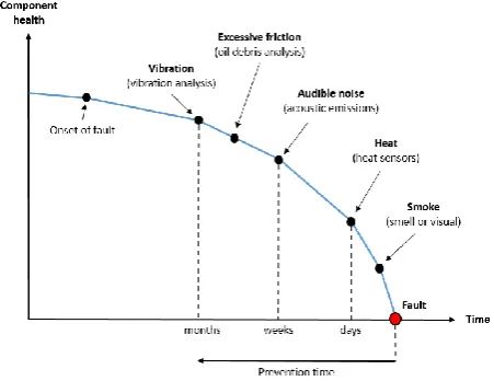
Faults in the generator can be both mechanical or electrical in nature, with the most common types of mechanical failure being due to mechanical looseness, misalignment and rotor imbalances within the system [6]. This investigation concentrates on a specific generator bearing failure, a mechanical looseness issue within the internal assembly. Mechanical faults all follow a similar path to failure regardless of the failure mode or root cause (see Figure 1). Once a fault has been introduced into the bearing the dynamic response of the system will change. This means that vibration analysis can sometimes be used to detect faults months before component failure, which allows for longer periods of time for wind farm operators to take preventative measures. Once a component gets closer to failure, excessive friction will be evident through oil debris analysis, before audible noise can detected either by ear or through acoustic emissions. The days leading up to failure heat and/or smoke will be detected indicating a serious incident could be imminent [7].

growth resulting in the bearing inner ring spinning on the generator rotor shaft at the drive end.

Figure 1: Diagram showing methods of detecting fault indicators over time as fault progresses towards failure. Adapted from [7].

3 Approach

In order to track and compare the component’s condition, vibration data was sought at different points in time leading up to generator bearing failure. To achieve this, events associated with generator bearing failure from a wind turbine OEM were analysed until 10-20 examples of the same failure mode were identified. This was then cross checked with SCADA data to ensure dates of wind turbine downtime were correlated. To guarantee a fair comparison, all examples were from an identical generator and drivetrain configuration; a doubly fed induction generator (DFIG) with a rated power of between 2-4 MW. Each turbine utilised a variable speed, pitch regulated control strategy. Generator rotor speed at rated power was determined by grid frequency, where examples were found for both 50 and 60 Hz.

Once the failure mode had been identified, the data gathered prior to occurrence was classified. Both a three and two class system were trialled, each divided into a number of categories based on health condition. Results from the two class system approach will be presented in this paper, which can be described as follows:

 Class 1: healthy - at least 5 months before failure

 Class 2: 1-2 months before failure

A total of 15 different wind turbines from eight wind farms were used in the study, in each of which the same failure mode was identified. Vibration data gathered consisted of at least six samples a week apart at 1 year, 5-6 months and 1-2 months before failure, with each turbine having data from at least two of the three classes. Each sample consisted of approximately 10 seconds of data taken with a sampling frequency of

approximately 25kHz at both the drive-end and non-drive end generator bearing (see Figure 2 for clarification).

Figure 2: Diagram showing rough accelerometer position used on generator bearings to measure vibration.

Once features were successfully identified and verified, machine learning algorithms were then trained and tested, with the most accurate chosen and applied to the set of features specific to the failure mode, classifying the condition according to whether it is healthy or not, and the time before failure. The algorithm was then tested against similar, unseen vibration data from wind turbines omitted from the training process. The prognostic process was evaluated, using a confusion matrix giving correct/incorrect classification and the likelihood of false positives/ negatives.

4 Vibration Analysis Techniques

Most of the experience to draw upon to analyse vibration in generators and other rotating machinery comes from industries which utilise large fixed speed machines. Modern wind turbines employ variable speed control strategies and, along with the stochastic nature of the wind, produce load patterns that are far more varied than traditional generators. The analysis of such vibration signals are therefore more complex and as such, makes diagnosing faults in wind turbine generators more difficult.

4.1 Time domain

Feature No.

Feature Formula

1 Maximum 𝑥𝑚𝑎𝑥 = max{x(t)}

2 Minimum 𝑥𝑚𝑖𝑛= min{x(t)}

3 Mean

𝑢𝑥=

1

𝑇∫ x(t)𝑑𝑡

𝑇

0

4 RMS

𝑢𝑟𝑚𝑠= [

1

𝑇∫ x

2_(t)𝑑𝑡

𝑇

0

] 1/2

5 Standard

Deviation 𝜎𝑥= [1

𝑇∫ [𝑥(t) − 𝑢𝑥]

2_𝑑𝑡 𝑇

0

] 1/2

6 Kurtosis

𝛽 =1

𝑇∫ [𝑥(t) − 𝑢𝑥]

4_𝑑𝑡 𝑇

0

Table 1: Time-domain features

4.2 Frequency domain

The frequency domain is one of the most commonly used methoda to analyse vibration in rotating equipment. Fourier analysis is a technique widely used to convert an input signal in the time domain to an output in the frequency domain using a fast Fourier transform (FFT) algorithm. The FFT algorithm samples a signal over a specific time period and divides it into its frequency components, with each sinusoidal component having a unique frequency with its own amplitude and phase. It is important to focus on the range of frequencies which are associated with the mechanical rotation of the generator shaft, which will allow any indicators of a fault to be detected. In general, this frequency range will be the mean generator shaft rotational frequency and associated harmonics.

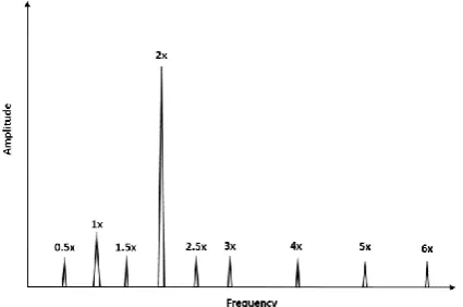
Figure 3: Expected harmonics and sub-harmonics introduced to the spectrum due to mechanical looseness within the internal generator assembly [6]

Consider a FFT spectrum of a vibration signal measured from an accelerometer located at a generator bearing with mechanical looseness in the internal assembly. Many harmonics are introduced into the spectrum due to the non-linear response of the loose parts to the exciting forces from the rotor, with the largest amplitude occurring twice per rotation (or 2× the shaft frequency). Sub-harmonics are often also caused at frequencies in multiples of 1/2 or 1/3 times the shaft

rpm (see Figure 3) [6]. The features extracted in the frequency domain are shown in Table 2.

Feature No.

Feature Description

1 1P Amplitude Amplitude of peak closest to mean shaft rotation

2 2P Amplitude Amplitude of peak closest to two times mean shaft rotation

3 1P Energy Energy in signal surrounding 1P

4 2P Energy Energy in signal surrounding 2P

Table 2: Frequency-domain features

4.3 Order domain

During each vibration sample the generator shaft speed varies, often significantly, meaning that the signal is not stationary. This produces a smearing effect on the FFT spectrum somewhat proportional to the range of shaft speeds experienced over the sample. One option available to try and negate these effects and gain a clearer picture of the signal is to perform order analysis. This is a resampling technique which takes a signal from the time domain, of constant sample rate at variable rotational speed, to the order domain, of variable sample rate at constant rotational speed.

Instead of frequency being represented along the x-axis (as with the FFT spectrum), the order domain uses order numbers, where the first order is a reference shaft speed. The order power spectrum is computed using a short-time Fourier transform of the resampled signal. Table 3 shows the features extracted from the order domain.

Feature No.

Feature Description

1 1st _order amplitude

Amplitude of peak at order number 1

2 2nd _order amplitude

Amplitude of peak at order number 2

Table 3: Order-domain features

5 Application of Fourier Analysis

understand which features can be extracted and more generally applied across any wind turbine.

Figure 4: Comparison of FFT spectra: same turbine, same health classification, similar operating points. Overlaid with frequencies of expected amplitude gains due to fault for clarity.

5.1 Comparison of similar operating conditions in the same wind turbine

The simplest comparison between spectra that can be made is by considering two different vibration samples of a single wind turbine when exposed to similar operating conditions within the same health classification. Figure 4 shows samples taken a week apart at similar wind speeds.

The first obvious observation is that the spectra are very similar in both peak amplitude and noise levels. The peak of the lower spectrum at 2× the rotational speed of the shaft is slightly lower and spread out, which can be attributed to higher variation in generator speed throughout the sample.

5.2 Comparison of different operating conditions in the same wind turbine

To show the influence that operating conditions have on the power spectrum, consider the same wind turbine (in the same health classification) but this time operating under significantly different external conditions. The first working in a region well below rated wind speed and the other considerably above. This comparison is shown in Figure 5.

The first notable observation is that the vibration signal measured when the turbine was operating above rated power has considerably more noise present. It also has a much lower and broader peak at 2× the rotational speed of the generator. This can be partly attributed to large variation in rpm of the high speed shaft. It is clear however that the energy contained in the signal surrounding this frequency is greater, meaning the peak in itself is not sufficient to determine if a fault is present.

Figure 5: Comparison of FFT spectra: same turbine, same health classification, different operating points. Below rated operating conditions (above) and above rated operating conditions (below). Overlaid with frequencies of expected amplitude gains due to fault for clarity.

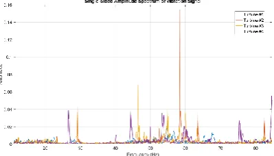
5.3 Comparison of different wind turbines in similar operating conditions.

Even with identical drivetrain configuration and performance specifications, the FFT power spectrum can change significantly between turbines. Figure 6 shows four examples, each taken from turbines with healthy generators in similar operating conditions. It should be noted that these turbines differ in design when it comes to the power output frequency, which would be 50Hz or 60Hz depending on the wind farm location globally. This will shift the operational speed of the high speed generator shaft, therefore shifting the frequency of any associated peaks in the FFT spectrum. It is clear that there is little coherence with regards to peak amplitude between turbines. This change in dynamics could be due to a range of factors: the manufacture and assembly of the drivetrain and wider structure, differences in fatigue and ageing of components due to structural and thermal loads, corrosion, faults and replacements elsewhere in the assembly, different wind profiles (shear and turbulence intensity) at a particular site, or even weather conditions at the time of measuring the vibration sample. Whatever the reasons, it is obvious that feature ranges or limits cannot be assumed equal for all turbines.

5.4 Comparison of spectra using the same turbine leading up to failure.

In order to determine whether features change as a generator bearing fault develops in a drivetrain, the FFT spectrum can be compared over time leading up to failure. Section 4 explains what should change in theory by introducing a fault associated with mechanical looseness, and by looking at multiple examples a sense of which features are actually observable in real wind turbine applications can be gained. Finding out to what extent these features are measurable (and in what time frame leading up to failure) is a useful exercise. Figure 7 shows examples of spectra for a wind turbine, with each classification presented leading up to failure.

The largest increase in amplitude occurs at approximately 58Hz (or 2× the rotational speed of the shaft), which is expected for a fault of this nature. It should be noted that the FFT amplitude in this example 1-2 months before failure is still lower than one of the healthy examples above, further proving that the dynamics are not the same for all turbines, even if identical machines.

The other expected gains in amplitude occur at shaft speed, and sub-harmonics at frequencies in multiples of 1/2 or 1/3 times the shaft rpm. In practise these gains are very hard to measure, and often not detectable.

Figure 7: Comparison of FFT spectra: same turbine, different health classification leading up to failure.

6 Application of Order Analysis

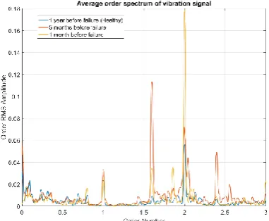
Figure 8 shows the same example used in Figure 7, but this time in the order domain as opposed to the frequency domain. When computing the frequency-RPM map it is important that a sensible resolution bandwidth is chosen to capture all the desired features of the signal therefore losing as little information as possible.

By applying order analysis techniques, the peaks at both 1x and 2× the shaft speed align, allowing for more clarity in the amplitude measurement. As the fault worsens and moves closer to absolute failure, the amplitude at 2× the shaft speed shows the most noticeable gain.

Figure 8: Comparison of order spectra: same turbine, different health classification leading up to failure.

7 Application of Support Vector Machine

Algorithms using Supervised Learning

Support vector machines (SVM) are adaptable algorithms widely used for both classification and regression problems. They work by plotting each data point in n-dimensional space, with n being the number of features used to train the model. Classification is achieved by finding the hyper-plane that differentiates the classes of coordinates (also known as support vectors). A simple example is shown in Figure 9. The margin is a measure of the distance between the hyper-plane and nearest support vector of each classification. A large margin indicates that the support vector machine is stable and will be less susceptible to misclassifying data [8].

Figure 9: Example of how support vector machines classify data.

There are two main stages when applying machine learning to vibration data for classification; a training phase followed by a validation phase. This process was repeated with different permutations of features to discover which could best be used to produce the greatest overall accuracy.

taken. Using a two class system, a total of 306 support vectors were established consisting of 204 in class A (healthy) and 102 in class B (1-2 months before failure). To ensure the algorithm is trained in a balanced manner, 100 random co-ordinates were chosen from each class.

Cross-validation was used to determine the overall accuracy of the algorithm. This method involves partitioning the data into subsets of a predetermined ratio, one of which is then omitted from training and used to test the algorithm. For this example, 20% of the data was used for validation purposes. The process is then repeated using different sup-populations and an average error calculated to use as a performance indicator.

8 Results

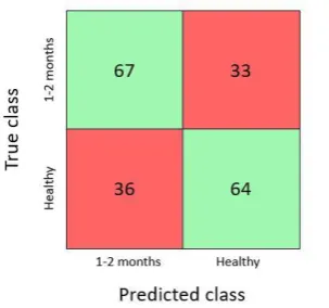
The accuracy of algorithm will depend on the random set of data which was taken for training and validation. By repeating this process, a mean accuracy can be determined along with associated standard deviation (see Figure 10). This will give a good indication of how sensitive and robust the algorithm is to the data used. A confusion matrix can be useful to visualise the algorithm accuracy by representing the true class and predicted class of each support vector, as shown in Figure 11.

Figure 10: Mean accuracy and standard deviation of algorithm variations using 7 random datasets.

Figure 11: Example confusion matrix using all features from a random set of training variables with 5-fold cross validation.

9 Conclusion

Predictive maintenance strategies that use previous failures to learn and predict failure and remaining useful life of different wind turbines have the potential to make substantial savings to costs associated with O&M. This research indicates that machine learning algorithms can be applied to specific features

to successfully predict generator bearing failure 1-2 months before occurrence with an overall accuracy of 67%. The example shown in Section 8 finds a balance between false-positives and false-negatives. From commercial perspective however, it may be worth refining the model to either minimise or maximise false-positives, which could be further explored through cost-benefit analysis.

Although the results shown in this paper seem reasonable, the accuracy is not great enough to effectively aid decision making. To further increase the accuracy beyond 70%, this generalised approach (training the model from any data within each health class) will need to be revised. Section 5 shows the differences which can occur in FFT spectra for different turbines, environmental conditions and operating points. A more specific training regime using sub-populations of data based on these factors could be one way to try and improve accuracy. In this case the methodology shown in this report could act as a starting point from with to refine as more information is learned about a specific wind turbine.

Acknowledgements

This work has been funded by the EPSRC, project reference number EP/L016680/1.

References

[1] C. Crabtree, D. Zappala, S. Hogg, Wind Energy: Uk experiences and offshore operational challenges, Power and Energy 2015, Vol. 229(7) 727746 IMechE 2015 [2] Bruce Valpy, Philip English, Future renewable energy

costs: offshore wind, KIC InnoEnergy, 2014

[3] F. Spinato, P. J. Tavner, G.J.W van Bussel and E. Koutoulakos, Reliability of wind turbine subassemblies, IET Renew. Power Generation, vol. 3, no. 4, pp. 1–15, Sep. 2009.

[4] James Carroll, Alasdair McDonald, David McMillan, Reliability study of wind turbines with DFIG and PMG drivetrains

[5] M. Wilkinson, K. Harman, F. Spinato, B. Hendriks, and T. Van Delft, Measuring Wind Turbine Reliability - Results of the Reliawind Project, in Proc. Eur. Wind Energy Conf., Brussels, Belgium, Mar. 14–17, 2011. [6] P. Girdhar and C. Scheffer, Practical Machinery

Vibration Analysis and Predictive Maintenance, Burlington, MA: Newnes, 2004.

[7] Pierre Tchakoua, etal, Wind Turbine Condition Monitoring: State-of-the-Art Review, New Trends, and Future Challenges, Energies 2014, 7, 2595-2630; doi:10.3390/en7042595