On the Existence and Uniqueness of the Eigenvalue
Decomposition of a Parahermitian Matrix
Stephan Weiss
, Senior Member, IEEE, Jennifer Pestana
, and Ian K. Proudler
Abstract—This paper addresses the extension of the factoriza-tion of a Hermitian matrix by an eigenvalue decomposifactoriza-tion (EVD) to the case of a parahermitian matrix that is analytic at least on an annulus containing the unit circle. Such parahermitian matrices contain polynomials or rational functions in the complex variable
zand arise, e.g., as cross spectral density matrices in broadband ar-ray problems. Specifically, conditions for the existence and unique-ness of eigenvalues and eigenvectors of a parahermitian matrix EVD are given, such that these can be represented by a power or Laurent series that is absolutely convergent, at least on the unit cir-cle, permitting a direct realization in the time domain. Based on an analysis of the unit circle, we prove that eigenvalues exist as unique and convergent but likely infinite-length Laurent series. The eigen-vectors can have an arbitrary phase response and are shown to exist as convergent Laurent series if eigenvalues are selected as analytic functions on the unit circle, and if the phase response is selected such that the eigenvectors are H¨older continuous withα > 12 on the unit circle. In the case of a discontinuous phase response or if spectral majorisation is enforced for intersecting eigenvalues, an absolutely convergent Laurent series solution for the eigenvectors of a parahermitian EVD does not exist. We provide some examples, comment on the approximation of a parahermitian matrix EVD by Laurent polynomial factors, and compare our findings to the solutions provided by polynomial matrix EVD algorithms.
I. INTRODUCTION
F
OR a multi-channel signal x[n]∈CM the instantaneous covariance matrix isR=Ex[n]xH[n], whereE{·} de-notes the expectation operator andxHrepresents the Hermitian transpose ofx. It captures the correlation and phase informa-tion on which rests the optimal soluinforma-tion of many narrowband array processing problems. For broadband signals, explicit de-lays must be considered instead of phase shifts, and capturingManuscript received August 31, 2017; revised December 31, 2017 and Febru-ary 16, 2018; accepted FebruFebru-ary 20, 2018. Date of publication March 6, 2018; date of current version April 17, 2018. The associate Editor coordinating the re-view of this manuscript and approving it for publication was Dr. Xavier Mestre. This work was supported in part by the Engineering and Physical Sciences Re-search Council, under Grant EP/K014307/1 and the MOD University Defence Research Collaboration in Signal Processing. (Corresponding author: Stephan
Weiss.)
S. Weiss is with the Centre for Signal and Image Processing, Department of Electronic and Electrical Engineering, University of Strathclyde, Glasgow G1 1XW, U.K. (e-mail: [email protected]).
J. Pestana is with the Department of Mathematics and Statistics, University of Strathclyde, Glasgow G1 1XW, U.K. (e-mail: [email protected]).
I. K. Proudler is with the Centre for Signal and Image Processing, Department of Electronic and Electrical Engineering, University of Strathclyde, Glasgow G1 1XW, U.K., and also with the School for Mechanical, Electrical and Man-ufacturing Engineering, Loughborough University, Leicestershire LE11 3TU, U.K. (e-mail: [email protected]).
Color versions of one or more of the figures in this paper are available online at http://ieeexplore.ieee.org.
Digital Object Identifier 10.1109/TSP.2018.2812747
the second order statistics can be accomplished via the space-time covariance matrix R[τ] =Ex[n]xH[n−τ] with a discrete lag parameterτ. SinceR[τ]contains auto- and cross-correlation terms ofx[n]it follows thatR[τ] =RH[−τ]. Tak-ing the z-transform leads to the cross spectral density (CSD) matrix1R(z) =
τR[τ]z−τ, which is a function of the com-plex variable z. The CSD matrix satisfies the parahermitian property R(z) =RP(z), where the parahermitian operation RP(z) =RH(1/z∗)involves Hermitian transposition and time reversal [1]. We call anyR(z)satisfying the parahermitian prop-erty a parahermitian matrix.
In the narrowband case, many optimal and robust solutions to signal processing problems rely on matrix decompositions [2], [3], particularly on the eigenvalue decomposition (EVD) ofR. To extend the utility of the EVD to the broadband case re-quires an equivalent factorisation of the parahermitian matrix R(z). Under the restriction ofR(z)having Laurent polynomial entries, a number of algorithms have been reported in the litera-ture over the past decade [4]–[12] that calculate an approximate polynomial EVDR(z)≈Uˆ(z)ˆΓ(z) ˆUP(z)consisting of Lau-rent polynomial factors, where Uˆ(z)is a paraunitary matrix, that is,Uˆ(z)satisfiesUˆ−1(z) = ˆUP(z)[1] andΓ(ˆ z)is a diago-nal polynomial matrix containing power spectral density (PSD) terms.
The above polynomial matrix EVD algorithms have proved useful in a number of applications, for example in denoising-type [13] or decorrelating array preprocessors [14], transmit and receive beamforming across broadband MIMO channels [15]– [17], broadband angle of arrival estimation [18], [19], optimum subband partitioning of beamformers [20], filter bank-based channel coding [21], fixed [22] and adaptive (i.e. minimum variance distortionless response) broadband beamforming [23], and blind source separation [24]. The polynomial approach can enable solutions that otherwise have been unobtainable: e.g. the design of optimal compaction filter banks beyond the two chan-nel case [8], the coherent estimation of broadband sources [19] without side-information, or the decoupling of dimensions and hence reduction of computational complexities of the quiescent beamformer, the blocking matrix and the adaptive noise can-celler in a polynomial generalised sidelobe cancan-celler [23].
1In our notation, boldface upper and lower case font refers to matrices and
vectors, respectively. A boldAgenerally refers to a time domain quantity, while A(z)is a transform domain quantity, withA(ejΩ)typically its evaluation on the unit circle,z= ejΩ.
Despite the numerous algorithms2and a number of success-ful applications, the theoretical foundations of the existence and uniqueness of a polynomial EVD have received little attention. The book by Gohberg et al. [25] considers the related factori-sation of a self-adjoint matrixA(x) =AH(x),x∈R, which can be applied to a parahermitian matrixR(z)on the unit circle via the reparameterisationz= ejΩ. Decompositions such as the Smith and Smith-MacMillan forms for matrices of polynomials and rational functions, respectively, are proven to exist [1], [25], but do not involve paraunitary and parahermitian factors as re-quired for the polynomial EVD in [4], [6]. Significantly, Icart and Comon [26] prove, based on known decompositions and the Stone-Weierstrass theorem, that the decomposition factors of a positive semi-definite parahermitian matrix can be approx-imated by Laurent polynomials. For the polynomial EVD in [9] and the related problem of a Laurent-polynomial QR decom-position [27], [28], the authors show that the factor matrices generally cannot exist as Laurent polynomials because the re-quired solutions involve divisions and square root operations of polynomials.
This paper aims to extend the work in [26] and to clarify the existence and uniqueness of factorising a parahermitianR(z) into paraunitary and diagonal parahermitian matrices. We gen-eraliseR(z)to include not just polynomials but rational func-tions inz∈C. Since the EVD even for a polynomialR(z)is not guaranteed to exist with Laurent polynomial factors [26], we refer to the decompositionR(z) =U(z)Γ(z)UP(z), with absolutely convergent Laurent series3U(z)andΓ(z)as a
para-hermitian matrix EVD (PhEVD). If it exists, the matrix of
eigen-values,Γ(z), is parahermitian and a Laurent series; the eigen-vectors inU(z)may exist as Laurent series, and, if causal, may even be power series. Absolute convergence—in some cases analyticity—of these factors will ensure that these Laurent or power series permit a direct time domain realisation. Our proof of existence and uniqueness proceeds in two stages. First, we characterize the PhEVD ofR(z)on the unit circle, i.e. in terms of the normalised angular frequencyΩ∈R. We next state the conditions that must be satisfied for the PhEVD factors to be representable as Laurent or power series. The main thrust of our analysis rests (i) on the analyticity ofR(z)[29] to guarantee that the CSD matrix is entirely characterised by its evaluation on the unit circle, (ii) on matrix perturbation theory [30], [31] to demonstrate the smooth evolution of EVD factors as functions ofΩ, and (iii) on complex function analysis [32] to extract con-vergent Laurent or power series. Throughout we assume that any eigenvalues of R(z)are non-negative for all |z|= 1and thatR(z)is analytic at least on an annulus containing the unit circle.
The paper is organised as follows. Section II provides back-ground on the existence and uniqueness of the EVD of a
2Many of these algorithms have convergence proofs, even though it is not
clear to which matrices they converge. 3The infinite sum
ncnz−n is a power series forn∈N, while for a Laurent seriesn∈Z. It does not need to converge to be called a series, but con-vergence criteria will be discussed later. Polynomials and Laurent polynomials are power and Laurent series, respectively, with a finite number of non-zero coefficientscn.
Hermitian matrix, and properties of and decomposition algorithms for parahermitian matrices. The parahermitian EVD problem is then mapped to the unit circle, i.e. |z|= 1, in Section III where we look at the conditions under which a func-tion of frequency admits a time series representafunc-tion. We then apply these results to the frequency domain EVD. This is first addressed in Section IV for the easier case thatR(z)has eigen-values of algebraic multiplicity one for all|z|= 1, i.e. when the eigenvalues are viewed in the Fourier domain as PSDs that do not overlap. Section V considers the case thatR(z)has, at least for somez on the unit circle, eigenvalues of algebraic multi-plicity greater than one. It generalises the findings of Section IV and contains the main results of this paper. A numerical example and a comparison with results obtained by iterative polynomial EVD algorithms are provided in Section VI, with concluding remarks in Section VII.
II. BACKGROUND
A. Eigenvalue Decomposition
We restrictR∈CM×M to be positive semi-definite—a prop-erty guaranteed ifRis e.g. a covariance matrix or emerges from a productR=AAH, with an arbitraryA∈CM×L. For any Hermitian matrixR=RH, its eigenvalue decomposition
R=QΛQH (1) exists, with the diagonal matrixΛcontaining the real-valued, non-negative eigenvaluesλm ∈R,m= 1. . . M, and the eigen-vectorsqm ∈CM, which we constrain to be orthonormal so that they form the columns of a unitary matrixQ.
While the EVD in (1) has unique eigenvalues, their sequence along the diagonal ofΛcan be arbitrary. This ambiguity w.r.t. a permutation can be removed by ordering eigenvalues inΛ in descending sequence,
λ1 ≥λ2 ≥ · · · ≥λM ≥0. (2) In the case ofM distinct eigenvalues, the eigenvectors ofRare unique except for a phase rotation. Ifqm is the eigenvector that corresponds to themth eigenvalueλm ofR, then
R qmejϕ =λmqmejϕ (3) holds for an arbitrary phase shiftϕ. Therefore, ifqm is anmth eigenvector, then so isqm =qmejϕ.
Ambiguity w.r.t. the eigenvectors also arises if eigenval-ues have an algebraic multiplicity greater than one, i.e. when the eigenvalues are no longer distinct. If λm =λm+1 =
. . . λm+C−1, these eigenvalues possess an algebraic multiplic-ity ofC and only theC-dimensional subspace containing the eigenvectors corresponding to this eigenvalue is uniquely de-fined, within which the eigenvectorsqm,qm+1, . . . qm+C−1 can form an arbitrary orthonormal basis: ifqm, . . . qm+C−1 are eigenvectors ofR, then so areqm, . . . qm+C−1,
[q
B. Parahermitian Space-Time Covariance Matrix
To understand how a parahermitian matrix may be obtained, we consider a scenario whereLindependent sources with non-negative, real power spectral densities (PSD)S(z),= 1. . . L, contribute toM sensor measurementsxm[n],m= 1. . . M. If these are organised in a vectorx[n] = [x1[n]. . . xM[n]]T, then the space-time covariance matrix is
R[τ] =Ex[n]xH[n−τ]. (5) If the PSD of theth source is generated by a stable and causal innovation filterF(z)[33], andHm (z)describes the transfer function of the causal and stable system between theth source and themth sensor, then
R(z) =H(z) ⎡ ⎢ ⎣
S1(z) . ..
SL(z) ⎤ ⎥
⎦HP(z) (6)
with the element in the mth row andth column of H(z) :
C→CM×L given by H
m (z), andS(z) =F(z)FP(z)the th element of the diagonal matrix of source PSDs.
The factorisation (6) can include the source model matrix F(z) =diag{F1(z), . . . , FL(z)}:C→CL×L, such that
R(z) =H(z)F(z)FP(z)HP(z). (7)
The components ofH(z)and the source modelF(z)are as-sumed to be causal and stable, and their entries can be either polynomials or rational functions inz. For the more general lat-ter case, let the maximum modulus of a pole of any component of eitherH(z)orF(z)beρ, where0< ρ <1. Thus the region of convergence forH(z)F(z)is |z|> ρ, while for the anti-causal termFP(z)HP(z)it is|z|< ρ−1. Overall, therefore, the CSD matrixR(z)in (7) can be represented as a Laurent series whose convergence regionDis the annulusρ <|z|< ρ−1[29], [34]. Hence, within this region, all entries ofR(z)are analytic and are therefore continuous and infinitely differentiable [29].
Since the PSDs satisfyS(z) =SP
(z), it is evident from both (6) and (7) that R(z) =RP(z) and so is parahermitian. The EVD of Section II-A can only diagonaliseR[τ]for one particu-lar lag valueτ, typically the Hermitian (narrowband) covariance matrix R[0]. The next section reviews efforts to diagonalise R(z)or, equivalently, diagonaliseR[τ]for all lagsτ.
C. Polynomial EVD
A self-adjoint matrix A(x), with x∈R, which satisfies A(x) =AH(x), has an EVD [30], [35] or spectral factorisa-tion [25], which can therefore describe the EVD ofR(z) evalu-ated on the unit circle, but not an EVD ofR(z)itself. The first mention of a polynomial EVD is in [4], which also proposed the second order sequential best rotation (SBR2) algorithm for its iterative approximation using Laurent polynomials. Over the past decade a number of algorithms have emerged [4], [6]–[12], [36], which share the restriction of considering the EVD of a parahermitian matrixR(z)whose elements are Laurent poly-nomials. In cases where the support is unknown or the source model in (7) contains rational functions, the auto- and
cross-correlation sequences in (5) may be estimated or approximated over a finite window of lags [8].
The polynomial EVD or McWhirter decomposition in [6] is stated as4
R(z)≈Uˆ(z)ˆΓ(z) ˆUP(z), (8) where the elements of the matrices on the r.h.s. are Laurent polynomials, Uˆ(z) is paraunitary and Γ(ˆ z) is diagonal and spectrally majorised, such that for the PSDs along the main diagonal,
ˆ
γm(ejΩ)≥γˆm+1(ejΩ) ∀Ω,
for m= 1. . .(M−1). Even though the term ‘polynomial EVD’ is not mentioned in [37], diagonalisation and spectral majorisation were introduced there in the context of optimising filter banks w.r.t. subband coding gain.
The approximation sign in the McWhirter decomposition (8) has been included in all subsequent algorithm designs over the past decade. Even though many algorithms can be proven to converge, in the sense that off-diagonal energy ofΓ(z)is re-duced at each iteration, see e.g. [6], [8], [10]–[12], and there is no practical experience yet where algorithms could not find a practicable factorisation, the only work towards the existence of the polynomial EVD has been reported in [26]. However, this provides limited understanding under which circumstances existence is guaranteed and does not address the uniqueness or ambiguity of eigenvalues and eigenvectors.
III. PARAHERMITIANMATRIXEVD
We first focus on the task of identifying the eigenvalues of a parahermitian matrix in the Fourier domain, and are particularly interested in determining how smoothly these vary, before in-vestigating the corresponding eigenvectors. Our approach rests on the conditions under which a function on the unit circle (i.e. a function of frequency) admits an absolutely convergent power or Laurent series, or even permits an analytic continuation to
z∈C, the ultimate aim being to find a suitable representation in the time domain.
A. EVD on the Unit Circle
We assume that the parahermitian matrix R(z) :C→
CM×M contains Laurent polynomials or rational functions inz, and is analytic in the annulusD={z:z∈C, ρ <|z|< ρ−1} with 0< ρ <1, as motivated in Section II-B. Since the unit circle is included in D, it follows from Cauchy’s integral for-mula that every value ofR(z)forρ <|z|<1is specified by its values for|z|= 1[34]. Because of the parahermitian property R(z) =RH(1/z∗), every value ofR(z)for1>|z|> ρ−1 is also specified by the values ofR(z)for|z|= 1. From a prac-tical aspect, the inverse z-transform requires evaluation on a closed path inD, which here can be the unit circle. This inverse transform leads back to the time domain, which then implies the
4The McWhirter decomposition in [6] is defined with the parahermitian
ˆ
existence of a Laurent seriesR(z) =τR[τ]z−τ: thusR(z) is recovered fromR(ejΩ). Therefore, in D,R(z)is uniquely characterised by R(ejΩ) =R(z)
z=ej Ω and vice versa, where
R(ejΩ)is Hermitian,R(ejΩ) =RH(ejΩ) ∀Ω.
An EVD ofR(ejΩ)can be evaluated at every point along the continuous normalised angular frequency variableΩ, such that
R(ejΩ) =Q(ejΩ)Λ(ejΩ)QH(ejΩ). (9)
At any arbitrary frequencyΩ, the properties of the EVD in (1) apply equally to (9), with the existence and uniqueness of its eigenvalues and -vectors as discussed in Section II-A. Since a parahermitian matrix is Hermitian on the unit circle it has real eigenvalues there.
B. Time-Domain Realisation
We want to form matrix functionsU(z)andΓ(z)as this will lead to a time domain representation and hence allow them to be implemented. The matrix functionsU(z)andΓ(z)need to matchQ(ejΩ)andΛ(ejΩ)in (9) at every frequency. There are infinitely many ways to do this. However we require a mech-anism that allows us to extract a direct realisation in the time domain of these functions on the unit circle i.e.Λ(ejΩ)→Γ[τ] andQ(ejΩ)→U[n], and this restricts the acceptable choices of U(z) andΓ(z). Ideally, we would like to extract analytic functionsΓ(z)andU(z), but we will be content if they can be represented by absolutely convergent power or Laurent series at least on the unit circle. Within their region of convergence, these functionsΓ(z)andU(z)are guaranteed to be unique [38], [39]. If an arbitrary 2π-periodic function X(ejΩ) :R→C has only a finite number of discontinuities, we can writeX(ejΩ) =
nx[n]ejΩn. For the Fourier coefficientsx[n]to represent an absolutely convergent Laurent or power series, we require abso-lute summability, i.e. n|x[n]|<∞. A sufficient condition for this is to restrict X(ejΩ) to be H¨older continuous with
α > 1
2 [40], such that
sup Ω1,Ω2∈R
|X(ejΩ1)−X(ejΩ2)| ≤C|ejΩ1 −ejΩ2|α (10)
with some C∈R. A continuous function X(ejΩ) is H¨older continuous if it does not behave too ‘wildly’. For the remainder of the paper, H¨older continuity always implies the condition
α > 1
2. In this case, the time domain realisation can be obtained by the inverse Fourier transform
x[n] = 1 2π
π
−π
X(ejΩ)ejΩndΩ. (11)
If, moreover,X(ejΩ)is analytic then we know that we can apply the inversez-transform
x[n] = 1 2πj
CX(z)z
ndz z
for C a closed counter-clockwise curve in the region of con-vergence ofX(z). ChoosingCto be the unit circle the inverse
z-transform becomes the inverse Fourier transform (11). Hence in this case the inverse Fourier transform can lead to a Laurent
seriesX(z) =nx[n]z−nthat is valid in an annulus with non-empty interior containing the unit circle. More generally, we can defineX(z) =nx[n]zn,|z|= 1from the Fourier series and attempt to analytically continue this representation. However, the region of convergence of the resulting series is difficult to determine.
Throughout, we use the terms “absolutely convergent power series” and “absolutely convergent Laurent series” to represent a power (Laurent) series that is absolutely convergent, at least on the unit circle. While there appears to be no simple necessary condition forX(ejΩ)to yield an absolutely convergent power or Laurent seriesx[n], a discontinuousX(ejΩ)is sufficient to exclude the existence of an absolutely convergent Fourier se-ries and hence of an absolutely convergent power or Laurent seriesx[n][40]. In general for the case of continuity, Weier-strass [41], [42] guarantees uniform convergence of a series of functions. These functions may change with the approximation order, hence it is neither possible to state a limit for infinite order using a power series, nor to obtain an approximation by truncation of that power series. Its use in this context is therefore limited. Therefore, the arguments in the remainder of this paper will focus on the H¨older continuity and potential smoothness of the factorsQ(ejΩ)andΛ(ejΩ)in (9).
C. Continuity of Eigenvalues
We now inspect how smoothly eigenvalues λm(ejΩ),m= 1. . . M, of R(ejΩ) in (9) evolve with the frequency Ω. To quantify the change that is induced in the eigenvalues of R(ej(Ω+ΔΩ)), withΔΩa small change in frequency, perturba-tion theory for matrices [30], [31] provides some useful results. The Hoffman-Wielandt theorem [43] shows that5
i
|λi(ejΩ)−λi(ej(Ω+ΔΩ))| ≤ R(ejΩ)−R(ej(Ω+ΔΩ))F, (12) assuming that the eigenvalues are ordered, with · Fthe Frobe-nius norm. Since based on the source model in Section II-B, R(z)is analytic and hence continuous,
lim ΔΩ→0R(e
jΩ)−R(ej(Ω+ΔΩ))
F = 0, (13)
which also implies continuity ofλm(ejΩ),m= 1. . . M, be-cause
lim ΔΩ→0
i
|λi(ejΩ)−λi(ej(Ω+ΔΩ))|= 0
must also hold on the l.h.s. of (12). Beyond continuity, analytic-ity ofR(z)on an annulus containing the unit circle ensures that the eigenvaluesλ1(ejΩ), . . . , λ
M(ejΩ)can be chosen to be an-alytic forΩ∈R[30], [35], and therefore can also be infinitely differentiable.6
5A regular perturbation ofR(z)can lead to either a regular or singular perturbation of the eigenvalues, but we are here only interested in the continuity of the latter.
6A similar frequency-domain approach for arbitrary matrices exists with the
D. Invariant Subspaces and Subspace Distance
Having characterized the eigenvalues ofR(z), we now turn to their corresponding eigenvectors, reviewing the effect of matrix perturbations on eigenvector subspaces. As highlighted in Sec-tion II-A, eigenvectors corresponding to multiple eigenvalues are not unique, and even though eigenvectors corresponding to tightly clustered eigenvalues are very likely ill-conditioned, the subspace spanned by these eigenvectors is usually insensitive to perturbations [31], [46].
Assume a cluster ofCadjacent (potentially multiple) eigen-values organised in the diagonal matrixΛ1(ejΩ) :R→RC×C, withΛ2(ejΩ) :R→R(M−C)×(M−C)containing the remaining
M−Ceigenvalues. The spread of the cluster is assumed to be small compared to the distanceδto the next-nearest eigenvalue outside this cluster [3], i.e.
max
λi,λj∈Λ1(ej Ω)|λi−λj| λ min
1 ∈Λ1(ejΩ)
λ2 ∈Λ2(ejΩ)
|λ1−λ2| ≡δ >0.
(14) The parameterδin (14) defines the spectral distance between the eigenvalues inΛ1(ejΩ)and inΛ2(ejΩ). IfQ
1(ejΩ) :R→
CM×C is a matrix whose columns are formed by theC eigen-vectors ofR(ejΩ)corresponding toΛ
1(ejΩ), andQ2(ejΩ)holds the remainingM−Ceigenvectors, we re-organise the EVD as QH(ejΩ)R(ejΩ)Q(ejΩ) =diagΛ1(ejΩ), Λ2(ejΩ) , (15) withQ(ejΩ) = [Q
1(ejΩ), Q2(ejΩ)]. Note that in accordance with (4), eigenvectors can have arbitrary phase shifts, which however does not affect the subspace analysis below.
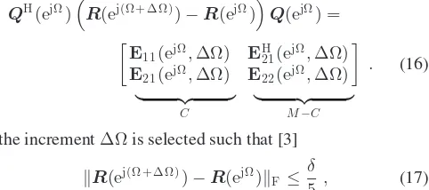
IfR(ejΩ)is perturbed by an increment in frequency,ΔΩ, then [3], [31]
QH(ejΩ)
R(ej(Ω+ΔΩ))−R(ejΩ)
Q(ejΩ) =
E11(ejΩ,ΔΩ) EH
21(ejΩ,ΔΩ) E21(ejΩ,ΔΩ) E22(ejΩ,ΔΩ)
. (16)
C M−C
If the incrementΔΩis selected such that [3]
R(ej(Ω+ΔΩ))−R(ejΩ)F≤ δ
5 , (17) i.e. such that the perturbation is small compared to the spectral distance δ, then for the two subspaces Q1(ejΩ) = rangeQ1(ejΩ)
andQ1(e(jΩ+ΔΩ)) =rangeQ
1(ej(Ω+ΔΩ))
dist{Q1(ejΩ),Q1(ej(Ω+ΔΩ))} ≤ 4δE21(ejΩ,ΔΩ)F . (18) The distance metric in (18) is defined as
dist{Q1(ejΩ),Q1(ej(Ω+ΔΩ))}=Π1(ejΩ)−Π1(ej(Ω+ΔΩ))2 =σmax ,
where · 2 is the spectral norm and Π1(ejΩ) = Q1(ejΩ)QH1(ejΩ) is the projection matrix onto the subspace
Q1(ejΩ)with0≤σmax ≤1[3].
Because of the continuity ofR(ejΩ)(see (13)) and the uni-tary invariance of the Frobenius norm, from (16) it follows
thatE21(ejΩ,ΔΩ)F −→0asΔΩ−→0. Hence the subspace evolves continuously. Interestingly, the distance between the subspaces spanned byQ1(ejΩ)andQ1(ej(Ω+ΔΩ))according to (18) is limited by the product of the perturbation-related term
E21(ejΩ,ΔΩ)
Fandδ−1. Therefore the subspace distance can increase as the distanceδto the nearest eigenvalue outside the cluster decreases.
E. Eigenvalue Considerations
The discussion in this section shows that different cases will arise depending on how we chooseΛ(ejΩ)andQ(ejΩ). An ar-bitrary frequency-dependent and potentially discontinuous per-mutationP(ejΩ)can be introduced into (9), such that
R(ejΩ) =Q(ejΩ)PH(ejΩ)P(ejΩ)Λ(ejΩ)PH(ejΩ)·
·P(ejΩ)QH(ejΩ). (19) Therefore, the resulting eigenvalues on the diagonal of P(ejΩ)Λ(ejΩ)PH(ejΩ) and eigenvectors in the columns of Q(ejΩ)PH(ejΩ)can be discontinuous. The statement of Sec-tion III-C thatΛ(ejΩ)can be continuous or even analytic for an
analytic R(z)implies that this permutation matrix is selected appropriately.7
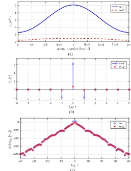
Based on the argument for at least continuous Q(ejΩ)and Λ(ejΩ)made in Section III-B, we here assume that permutations are chosen such that eigenvalues are at least continuous on the unit circle, i.e. that permutations of eigenvalues can only occur at algebraic multiplicities of those same eigenvalues, and are applied such that2π-periodicity of all functions in (19) is retained. In the following we therefore distinguish three cases as characterised by the examples in Fig. 1:
a) non-overlapping eigenvalues λm(ejΩ), where all eigen-values have algebraic multiplicity one for all frequencies Ω, such as the PSDs shown in Fig. 1(a);
b) overlapping, maximally smooth eigenvalues, such as shown in Fig. 1(b); and
c) overlapping, spectrally majorised PSDs as shown in Fig. 1(c).
Note that cases (a) and (c) are spectrally majorised, while cases (a) and (b) will be seen to yield analytic eigenvalues forΩ∈
R. Note that not all eigenvalues in (c) are differentiable for every value of Ω, but they will later shown to be Lipschitz continuous. In the rest of this paper we treat the cases of distinct and overlapping eigenvalues separately.
IV. CASE OFDISTINCTEIGENVALUES
In the case of distinct, non-overlapping eigenvaluesλm(ejΩ),
m= 1. . . M, spectral majorisation in (2) holds with strict in-equality for allΩ. As a result, the power spectra of the eigenval-ues are smooth and distinct and, as in the example of Fig. 1(a), do not intersect.
7Recall from Section III-B that a discontinuous function of frequency will
[image:5.594.48.289.449.556.2]Fig. 1. Examples for (a) non-overlapping and overlapping eigenvalues with (b) smooth and (c) spectrally majorised PSDs. Non-differentiable points are indicated by black circles.
A. Existence, Uniqueness and Approximation of Eigenvalues
Theorem 1 (Existence and Uniqueness of Distinct Eigenval-ues): LetR(z)be a parahermitian matrix which is analytic at least on an annulus containing the unit circle and whose EVD on the unit circle, as defined in (9), has distinct eigenvalues
λm(ejΩ),∀Ωandm= 1. . . M. Then a matrix of eigenvalues of R(z) exists as a unique analytic Laurent series Γ(z)that matchesΛ(ejΩ) =diagλ
1(ejΩ). . . λM(ejΩ)on the unit cir-cle.
Proof: IfR(z)is analytic in the annulusρ <|z|< ρ−1 then we know from Section III-C that the eigenvalues λm(ejΩ),
m= 1, . . . , M can be chosen to be analytic for realΩ. Since analytic functions are H¨older continuous the discussion in Sec-tion III-B applies and therefore a potentially infinite order, matrix-valued Fourier series can be found that converges to Λ(ejΩ). Further since the eigenvalues are analytic on the unit circle, the Fourier series representation of the eigenvalues can be analytically continued to an annulus containing the unit circle via the substitutionz= ejΩ. This gives the potentially infinite Laurent seriesΓ(z)representing theM eigenvalues ofR(z). This matrix of eigenvalues,Γ(z), matches Λ(ejΩ)on the unit circle, and therefore is unique as discussed. In order to find an approximation of finite length to a Laurent or power series, consider that the Fourier series of the mth eigenvalue takes the formλm(ejΩ) = limN−→∞λˆmN(ejΩ), with
ˆ
λmN(ejΩ) = N
=0
cm ,ejΩ+c∗m ,e−jΩ, cm ,∈C. (20)
WithΛˆN(ejΩ) =diagˆλN
1 (ejΩ), . . . ,ˆλ N
M (ejΩ)
, absolute convergence implies uniform convergence, such that for every
Λ >0there existsN >0with
sup Ω∈[0,2π)
ΛˆN(ejΩ)−Λ(ejΩ) <
Λ, (21)
where · is any matrix norm. As N → ∞, Λ →0 at ev-ery frequencyΩ, so that the Fourier series (21) converges to Λ(ejΩ). For finiteN, an analytic continuation via the substitu-tionz= ejΩ into (20) is always possible, and yields a Laurent polynomial approximationΓ(ˆ z). Alternatively, a direct approx-imation ofΛ(ejΩ)by Laurent polynomials is available via the Stone-Weierstrass theorem [41], [42], [47].
When approximating the exact eigenvaluesΓ(z)by Laurent polynomials of order2N, a truncation error is incurred accord-ing to (21). Since the region of convergence ofΓ(z)may be smaller thanD, we cannot make a statement here about how fast or slow such an approximation converges. The generally infinite-length nature of the Laurent series representation of the eigenvalues will be evident when we consider the “simple” case of a2×2parahermitian matrix next, followed by an example problem that was stated but not solved in [26].
B. Eigenvalues of2×2Parahermitian Matrices
In this section we exemplify the existence and uniqueness of the eigenvalues of an arbitrary parahermitian matrixR(z) :
C→C2×2. These eigenvaluesγ
1,2(z)can be directly computed in thez-domain as the roots of
det{γ(z)I−R(z)}=γ2(z)−T(z)γ(z) +D(z) = 0
with determinant D(z) = det{R(z)} and trace T(z) = trace{R(z)}. This leads to
γ1,2(z) = 1 2T(z)±
1 2
T(z)TP(z)−4D(z). (22)
The argument under the square root is parahermitian and can be factored intoY(z)YP(z) =T(z)TP(z)−4D(z), whereY(z) has all zeros and poles inside the unit circle, andYP(z)has all zeros and poles outside the unit circle. In the rare case that
Y(z)has no poles and all zeros have multiplicity2N,N∈N, the solution for (22) is a Laurent polynomial. If both poles and zeros ofY have multiplicity2N,N ∈N, the eigenvalues are rational functions inz.
In general, the square root in (22) will be neither polyno-mial nor rational, as recognised for a Laurent polynopolyno-mial QR decomposition in [27]. Within the convergence region|z|> ρ, whereρ <1is the maximum modulus of all poles and zeros of
Fig. 2. MacLaurin series expansion coefficients for square root of a zero or pole.
separately. Then a Maclaurin series expansion gives
1−βz−1= ∞
n=0
ξnβnz−n (23)
1
√
1−αz−1 = ∞
n=0
ξnαnz−n −1
(24)
= ∞
n=0
χnαnz−n (25)
with
ξn = (−1)n 1
2
n
=(−1) n n!
n−1
i=0
1 2 −i
,
χn = (−1)n
−1 2
n
= (−1) n−1
n! n−1
i=0
1 2 +i
.
The MacLaurin coefficients ξn and χn for n= 0. . .50 are shown in Fig. 2.
Thus, a stable causal square rootY(z)1/2 is obtained. The square root ofYP(z)with a convergence region |z|< ρ−1 is given by YP(z)!1/2 = Y(z)1/2!P. The representation of the square root is therefore complete, and can be accomplished by an infinite order rational function in z via (23) and (24), or by a Laurent series via (23) and (25). The eigenvalues in (22) therefore exist as convergent but generally infinite Laurent series [41] but clearly could be approximated by finite order rational functions or Laurent polynomials.
Example. To demonstrate the calculation of eigenvalues, we
consider the parahermitian matrix
R(z) =
1 1
1 −2z+ 6−2z−1
(26)
stated in [26], which has poles at z= 0 and z→ ∞ but is analytic in{z:z∈C, z= 0,∞}.
Using (23) and (25), the approximate Laurent polynomial eigenvalues are characterised in Fig. 3 in terms of their PSDs ˆ
γm(ejΩ), expansion coefficients ˆγm[τ] such that γˆm(z) =
τˆγm[τ]z−τ, and their log-moduli. The latter in Fig. 3(c) shows the rapid decay of the Laurent series, justifying a Laurent polynomial approximation.
This expands on the result in [26], where it was shown that R(z)in (26) does not have polynomial eigenvalues, but where
Fig. 3. Approximate eigenvalues ofR(z)in (26). (a) Power spectral densities. (b) Laurent polynomial coefficients. (c) Decay of power series.
no polynomial or rational approximation was given. The ex-ample demonstrates that an approximate solution using Laurent polynomials exists, which can be arbitrarily accurate for a suf-ficiently high order ofˆγ1,2(z), as supported by Theorem 1.
C. Existence, Ambiguity and Approximation of Eigenvectors
Recall that the eigenvalues ofR(ejΩ)are assumed to possess non-overlapping PSDs, i.e the eigenvalues for all frequencies Ω have algebraic multiplicity one, i.e.C= 1. The subspaces in Section III-D can now all be treated as one-dimensional, and eigenvectors are therefore uniquely identified, save for the phase shift in (3). Since this phase shift is arbitrary at every frequencyΩ, the polynomial eigenvectors are defined up to an arbitrary phase response. With this, some of the expressions in Section III-D simplify, and permit the statement of the following theorem.
[image:7.594.41.288.67.166.2]Proof: Considering themth eigenvalue and -vector,λm(ejΩ) andqm(ejΩ), the spectral distance from its nearest neighbour at frequencyΩis [31]
δm(ejΩ) = minn =m|λn(e
jΩ)−λ
m(ejΩ)|>0.
Now, in (16),E21(ejΩ) :R→CM−1 is a vector, and if (17) holds, then (18) simplifies to
dist{qm(ejΩ),qm(ej(Ω+ΔΩ))} ≤ δ 4
m(ejΩ)E21(e
jΩ,ΔΩ) F .
AsΔΩ−→0, alsodist{qm(ejΩ),qm(ej(Ω+ΔΩ))} −→0, and the one-dimensional subspace within which each eigenvector re-sides must evolve continuously with frequency. It can be further shown that the eigenvectors can be chosen to be analytic [35].
Because of the phase ambiguity in (3), each eigenvec-tor can be given an arbitrary phase response Φm(ejΩ), with
|Φm(ejΩ)|= 1∀Ω∈[0; 2π), m= 1. . . M without affecting the orthonormality of eigenvectors. Only ifΦm(ejΩ)is selected such that theMelements ofqm(ejΩ)vary H¨older-continuously inΩ, then analogously to the proof of Theorem 1, a H¨older-continuousqm(ejΩ)has an absolutely convergent Fourier se-ries [40]
ˆ
qmN(ejΩ) = N
=−N
dm ,·ejΩ, (27)
where dm ,∈CM andˆqmN(ejΩ)−qm(ejΩ) −→0 ∀Ω as N −→ ∞. According to Section III-B, this admits an absolutely convergent power or Laurent seriesum(z). If additionally the phase response does not just create aqm(ejΩ)that is H¨older con-tinuous but one that is also analytic inΩ, then the continuation
to an analyticum(z)exists.
The selection of the phase response does not just cause am-biguity of the eigenvectors, but also affects the properties of a Laurent polynomial approximation of these eigenvectors. An appropriate phase response may e.g. admit a causal, polyno-mial approximation. Further, we distinguish below between the selection of a continuous and a discontinuous phase response, leading to matricesQ(ejΩ)that are continuous and discontinu-ous inΩ, respectively:
r
H¨older Continuous Case. This case is covered byTheo-rem 2, which requires phase responses that are otherwise arbitrary but constrained for qm(ejΩ), m= 1. . . M, to be H¨older continuous for eigenvectorsU(z) to exist as convergent Laurent or power series. Ambiguity w.r.t. the phase response implies that for any differently selected continuous phase response, a differentU(z)emerges. Ap-proximations ofU(z)by Laurent polynomialsUˆ(z)can be obtained by truncation; this approximation will improve with the approximation order and smoothness of the phase response. A special case arises if the phase responses are selected such thatQ(ejΩ)is analytic, which directly im-plies a convergent power seriesU(z).
r
Discontinuous Case. If qm(ejΩ) is piecewise continu-ous and possesses a discontinuity atΩ = Ω0, then there does not exist a convergent Laurent or power seriesrepresentation of the eigenvector. However sinceqm(ejΩ) is periodic inΩ, an at least pointwise convergent Fourier series does exist, and at the pointΩ0will converge to
lim N→∞ˆq
N
m (ejΩ0) = 12Ωlim→0
qm(ej(Ω0−Ω)) +
+ qm(ej(Ω0+Ω))
. (28)
Since (28) is the mean value between the left- and right function values at the discontinuity, a Fourier series rep-resentation will not matchqm(ejΩ)at least atΩ0. An ap-proximation by a Laurent polynomialUˆ(z)of sufficiently high order, evaluated on the unit circle, will converge to the mean values ofQ(ejΩ)according to (28) at the disconti-nuities, and Gibbs phenomena may occur in the proximity. For the case where eigenvalues qm(ejΩ) are neither H¨older-continuous nor disH¨older-continuous, uniform convergence of the Fourier series cannot be guaranteed [40]; this case is outwith the scope of this paper, but we refer the interested reader to e.g. [40] for the appropriate conditions on convergence.
V. CASE OFEIGENVALUESWITHMULTIPLICITIES
Following the consideration of distinct, non-overlapping eigenvaluesλm(ejΩ),m= 1. . . M, in Section IV, we now ad-dress the case where the PSDs of eigenvalues intersect or touch, i.e. there is an algebraic multiplicity of eigenvalues greater than one at one or more frequencies. Because of an ambiguity of how to associate eigenvalues across the frequency spectrum, similar to the permutation problem in broadband blind source separation, a distinction is made between maximally smooth and spectrally majorised PSDs, as illustrated by the examples in Fig. 1(b) and (c), respectively.
A. Existence, Uniqueness and Approximation of Eigenvalues
Section III-C indicated that eigenvalues ofR(ejΩ), that have an algebraic multiplicity of one, can be chosen to be analytic (hence continuous and infinitely differentiable) functions on the unit circle [35]. Therefore if we constrain the eigenvalues to be continuous, thenΛ(ejΩ)has to be at the very least piecewise analytic on the unit circle.
It follows that if any two eigenvaluesλm(ejΩ)andλ n(ejΩ), m, n= 1. . . M, are permuted at an algebraic multiplicity greater than one, then
sup Ω1,Ω2∈R
|λm(ejΩ1)−λ
n(ejΩ2)| ≤L|ejΩ1 −ejΩ2|
holds withm, n= 1. . . M, the Lipschitz constant
L= max
m∈ {1,2, . . . M} Ω∈R\ M
""
""dΩd λm(ejΩ)"""" , (29)
Fig. 4. Cluster ofCeigenvalues in the neighbourhood of aC-fold multiplicity atΩ = Ω0.
Hence, this is a stronger condition than H¨older continuity, and therefore guarantees the representation by an absolutely conver-gent Fourier series in analogy to the arguments in Section IV-A; an alternative representation in terms of Laurent series can be reached via the Stone-Weierstrass theorem. This leads to the following theorem:
Theorem 3 (Existence and uniqueness of eigenvalues of a parahermitian matrix EVD): LetR(z)be an analytic paraher-mitian matrix whose EVD on the unit circle, as defined in (9), has an eigenvalue matrixΛ(ejΩ),∀Ω∈R. Then the matrix of eigenvalues Γ(z) exists as an absolutely convergent Laurent series. Uniqueness requires additional constraints on the per-mutation of eigenvalues on the unit circle, such as maximal smoothness or spectral majorisation, with consequences for the order of a Laurent polynomial approximationΓ(ˆ z)ofΓ(z).
Proof: This is covered by Theorem 1 for distinct eigenvalues,
and otherwise follows from the above reasoning. The approximation of eigenvalues by Laurent polynomials, here argued in terms of a truncated Fourier series expansion (see Theorem 1), is guaranteed to be analytic because of the restriction to a finite order. However, differences in the con-vergence speed can be noted: we expect faster concon-vergence for analytic, i.e. maximally smooth eigenvalues than for spectrally majorised ones, since for the latterΛ(ejΩ)is only piecewise an-alytic on the unit circle. Therefore generally higher order Lau-rent polynomials are required when approximating spectrally majorised eigenvalues as compared to the maximally smooth case, if eigenvalues have an algebraic multiplicity greater than one on the unit circle. This outcome of Theorem 3 agrees with results in [9], as well as with experimental findings in [48] based on factorisations for different source models—with both distinct and spectrally majorised sources—of a space-time covariance matrix.
B. Uniqueness and Ambiguity of Eigenvectors
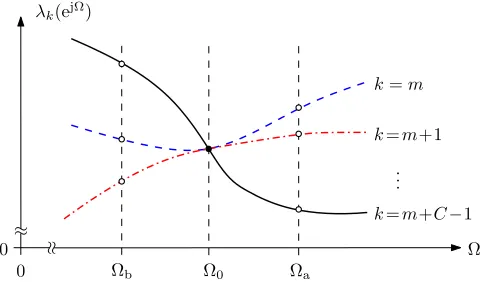
We now inspect the eigenvectors in the vicinity of a
C-fold algebraic multiplicity of eigenvalues at Ω = Ω0, as shown in Fig. 4. By assumptionR(ejΩ)is analytic and, from Section III-C, Λ(ejΩ) can be chosen to be analytic for all Ω, including Ω0. In this case, Rellich [35] shows that the
eigenvectors can be analytic. We want to explore the behaviour ofQ(ejΩ), and particularly the conditions under which it has a unique analytic solution. That this is the case seems to be under-stood in various texts [30], [35], [45] but the authors have not found a definitive reference. Hence we offer Lemma 1, below, as an alternative proof.
In rare cases we may find identical eigenvalues. Two eigenvalues λm(ejΩ)and λ
(ejΩ) are identical if λm(ejΩ) = λ(ejΩ)∀Ω. In the following we exclude this case; an ambigu-ity is expected from (4), but the presence of identical eigenvalues makes the analysis more involved and the case is usually avoided by estimation and rounding errors inR(z).
Lemma 1 (Existence and uniqueness of analytic eigenspaces on the unit circle): Under the assumptions of Theorem 3 and
in the absence of identical eigenvalues, there exist unique 1-d subspaces for analytic eigenvectors in Q(ejΩ)if and only if eigenvalues inΛ(ejΩ)are selected to be analytic across alge-braic multiplicities.
Proof: That it is possible to choose analytic eigenvectors
when the eigenvalues are all chosen to be analytic follows from Rellich [35]. To see the ‘only if’ part, we now assume that the eigenvectors are chosen to be analytic, and show that this can only occur if the eigenvalues are also analytic.
By exploiting Theorem 1 between multiplicities, we know that continuous eigenvalues have to be at the very least piece-wise analytic on the unit circle. Further, between the points of multiplicity greater than one, these functions are unique (up to the order they appear in the matrixΛ(ejΩ)). If the analytic eigenvalues from Rellich areΛ0(ejΩ), then the only alternative choice for the eigenvalue matrix is
Λ(ejΩ) = #
Λb(ejΩ) =PbΛ0(ejΩ)PH
b, Ω≤Ω0, Λa(ejΩ) =PaΛ0(ejΩ)PH
a, Ω≥Ω0, (30)
where subscripts ‘a’ and ‘b’ indicate ‘above’ and ‘below’Ω0, and Pa,Pb∈RM×M are permutation matrices. Because we can arbitrarily order the eigenvalues inΛ0(ejΩ)and their corre-sponding eigenvectors inQ(ejΩ)without affecting their analyt-icity, w.l.o.g. we setΛa(ejΩ) =Λ0(ejΩ), i.e. Pa =I.
With reference to (19), we have
R(ejΩ) = #
Q(ejΩ)Λb(ejΩ)QH(ejΩ), Ω≤Ω0 , Q(ejΩ)Λa(ejΩ)QH(ejΩ), Ω>Ω0 , (31)
where Q(ejΩ)is assumed to be analytic, and R(ejΩ) is ana-lytic by premise. With this, we can definenth order derivatives approachingΩ0from above and below,
lim Ωa−→Ω0+
dn dΩna
R(ejΩa) =R(n)
a , (32)
lim Ωb−→Ω0−
dn dΩnb
R(ejΩb) =R(n)
b , (33)
above and below Ω0 analogously to (32) and (33). Note that because of the analyticity ofQ(ejΩ),Q(n)
a =Q(bn) ∀n∈N. For R(0)a =R(0)b , we take the EVD on either side, and withQ(0)a =Q(0)b and the premise of continuous eigenvalues, i.e. Λ(0)a =PHbΛ
(0)
b Pbdue to (30), obtain
Q(0)b PHbΛ(0)b PbQ (0),H b =Q
(0) b Λ
(0) b Q
(0),H
b . (34) or
PH bΛ
(0) b Pb−Λ
(0)
b =0. (35)
For the first derivativeR(1)a , the product rule can be applied to the EVD factorisation,
R(1)
a =Q(1)a Λ(0)a Q(0)a +Q(0)a Λ(1)a Q(0)a +Q(0)a Λ(0)a Q(1)a .
Taking the derivative of the r.h.s. of (34) and using a similar expression forR(1)b , and equatingR(1)a =R(1)b , we find that
Q(1) b
PH
bΛ(0)b Pb−Λ (0) b
Q(0),H
b +
+ Q(0)b
PH bΛ
(0) b Pb−Λ
(0) b
Q(1),H
b +
+ Q(0)b
PH
bΛ(1)b Pb−Λ (1) b
Q(0)b ,H = 0.
Because of (35), the first two terms are zero, and we obtain PH
bΛ (1) b Pb−Λ
(1)
b =0. By induction it can be shown that for R(n)
a =R(bn) indeedPHbΛ (n) b Pb−Λ
(n)
b =0∀n∈N, or Λ(n)
b Pb−PbΛ (n)
b =0 ∀n∈N. (36) Ifpm , is the element in themth row andth column ofPb, then elementwise, (36) demands
pm ,
λ(n) b, −λ
(n) b,m
= 0 ∀n∈N, withλ(bn,m) themth diagonal entry ofΛ(bn).
In the absence of identical eigenvalues, even if theth and
mth eigenvalues,m, ∈ {1. . . M},m=, belong to the clus-ter forming aC-fold algebraic multiplicity atΩ0, they will differ in at least one differentiationn, and hencepm , = 0. As an ex-ample, in Fig. 4, the 0th and 1st order derivatives ofλm(ejΩ)and
λm+1(ejΩ)match atΩ = Ω0, but then= 2nd order derivatives differ. Therefore,Pb must be a diagonal matrix. Further, uni-tarity, and the fact thatPbis a permutation matrix enforces the constraintpm ,m = 1,m= 1. . . Mi.e.Pb =I. Thus from (30), recalling thatPa =I, we must haveΛ(ejΩ) =Λ0(ejΩ). There-fore analytic eigenvectors are possible if and only if eigenvalues are analytically continued acrossΩ0.
Recall that the eigenvectors inQ(ejΩ)can possess arbitrary phase responses; as long as the latter are analytic,Q(ejΩ)will remain analytic. While this permits some ambiguity, under the exclusion of identical eigenvalues, each eigenvector must how-ever be orthogonal to the remaining eigenvectors, and hence there exist unique 1-d subspaces within which analytic
eigen-vectors reside.
Analyticity or at least H¨older continuity ofQ(ejΩ)requires that Λ(ejΩ)is analytic, and that the arbitrary phase response of Q(ejΩ) is selected analytic or at least H¨older continuous.
We focus next on extending the eigenvalues and eigenvectors to functions inz.
Theorem 4 (Existence and ambiguity of eigenvectors of a parahermitian EVD): IfR(z)has no identical eigenvalues, then there exist unique 1-d subspaces for analytic eigenvectors of a parahermitian matrix EVD, if and only if the eigenvalues are analytic across a potential algebraic multiplicity greater than one on the unit circle. Within this 1-d subspace, an eigenvector exists as a convergent Laurent or power series if its arbitrary phase response is selected such that the resulting eigenvectors are H¨older continuous in frequencyΩ.
Proof: It is known that the eigenvectors can be chosen to
be analytic on the unit circle if and only if the eigenvalues are (e.g. Lemma 1). Each eigenvectorqm(ejΩ),m= 1, . . . , M, can always be multiplied by an arbitrary phase responseΦm(ejΩ), provided|Φm(ejΩ)|= 1for allΩ. If this phase response creates an eigenvectorqm(ejΩ)that is H¨older continuous for allΩ, then
qm(ejΩ)can be represented by an absolutely convergent Fourier series as in (27). Analogous to the proof of Theorem 3, therefore an absolutely convergent power or Laurent seriesum(z)exists as the eigenvector, which matchesqm(ejΩ)on the unit circle, i.e.
um(z)|z=ej Ω =qm(ejΩ). The selection of the phase response
will have an impact on the causality ofum(z), i.e. whether it
will be a power or Laurent series.
If the phase response is selected more strictly such that qm(ejΩ) is not just H¨older continuous but analytic, then an analytic um(z) can be obtained by analytic continuation via z= ejΩ [29], [38], [39].
As a converse to Theorem 4, when eigenvalues are not se-lected analytic on the unit circle, e.g. by enforcing spectral majorisation in the case of an algebraic multiplicity of eigen-values greater than one on the unit circle, or in the case of ana-lytic eigenvalues but a discontinuous phase responseΦm(ejΩ), discontinuous eigenvectors qm(ejΩ)arise for which no exact representation by an absolutely convergent power or Laurent series exists.
C. Approximation of Eigenvectors
It is clear that if all eigenvectorsqm(ejΩ),m= 1. . . M are H¨older continuous by virtue of analytic eigenvaluesλm(ejΩ) and appropriate phase responses, the convergent Laurent or power seriesU(z)can be approximated arbitrarily closely by Laurent polynomialsUˆ(z)—or polynomials in the case that the phase response admits a causalUˆ(z)—analogously to (21). The speed of convergence depends on the smoothness ofQ(ejΩ), with faster convergence for smoother functions. The fastest convergence can be expected if Q(ejΩ) is analytic, the con-ditions for which are given by Rellich [35] and highlighted in Lemma 1 (see Section V-B.)
For the following cases, Theorem 4 could not prove the ex-istence of absolutely convergent power or Laurent series as eigenvectorsU(z). Nevertheless, approximations may still be found:
r
Discontinuous Phase Response. For analytic eigenvalues,approximation Uˆ(z)can be reached via a Fourier series which on the unit circle converges to Q(ejΩ) except at these discontinuities. At discontinuities, the approxima-tionUˆ(z)|z=ej Ω will converge to the average values stated
in (28).
r
Spectrally Majorised Eigenvalues. If eigenvalues have analgebraic multiplicity greater than one on the unit circle, discontinuities arise for the corresponding eigenvectors qm(ejΩ). Provided that these, together with any discon-tinuities introduced by the phase responses, are finite in number, a polynomial or Laurent polynomial approxima-tionUˆ(z)via a Fourier series obeying (28) can be found.
VI. NUMERICALEXAMPLE
We provide results for a numerical example with known ground truth for a PhEVD with both analytic and spectrally majorised eigenvalues, as well as for the results obtained by the SBR2 algorithm [6]. This informs observations on differences between the theoretical PhEVD established in terms of its exis-tence and uniqueness in this paper, and what is obtainable via iterative polynomial EVD algorithms.
ConsiderR(z) =U(z)Γ(z)UP(z)with paraunitaryU(z) = [u1(z),u2(z)]andu1,2(z) = [1,±z−1]T/
√
2. With the diagonal and parahermitianΓ(z) =diagz+3+z−1;−jz+3+jz−1, the parahermitian matrixR(z) :C→C2×2 is
R(z) = $1−j
2 z+ 3 + 1+j
2 z−1 1+j
2 z2+ 1−j
2 1+j
2 +1−2jz−2 12−jz+ 3 + 1+j2 z−1 %
. (37)
Analytic / Maximally Smooth Case. When extracting
eigen-values that are analytic on the unit circle, the so-lution is given by the diagonal elements of Γ(z) = diag[z+ 3 +z−1; −jz+ 3 + jz−1], which are taken from an example in [26]. The two eigenvalues overlap atΩ = 1
4πand Ω =5
4π, where they have an algebraic multiplicity of two, as shown in Fig. 5(a).
The two eigenvectorsu1,2(z) = [1,±z−1]T/
√
2are of order one. To show that their evaluation on the unit circle evolves smoothly with frequencyΩ, we defineϕm(ejΩ)as the Hermi-tian subspace angle [49], [50] relative to the arbitrary reference vectoru1(ej0),
cosϕm(ejΩ) =|uH1(ej0)um(ejΩ)|, (38) withm= 1,2and0≤ϕm(ejΩ)≤ π2. Similar to the subspace distance discussed in Section III-D, in the absence of an alge-braic multiplicity of eigenvalues greater than one, these angles can be shown to evolve continuously under sufficiently small perturbations ofR(z)[51]–[53].
Fig. 5(b) shows the subspace angles in (38), and indicates their smooth evolution with frequency. Note that because of the modulus operation involved in the Hermitian angles, the latter are reflected atϕ= 0andϕ= π2, making ϕ(ejΩ) non-differentiable even though the eigenvectors themselves can be differentiated w.r.t.Ω.
Ideal Spectral Majorisation. To achieve spectral
[image:11.594.307.547.64.261.2] [image:11.594.307.547.306.503.2]majorisa-tion, the eigenvalues of the analytic case have to be permuted on the frequency interval Ω = [14π, 54π] as shown in Fig. 6(a).
[image:11.594.46.288.375.408.2]Fig. 5. (a) PSDs of eigenvalues that are analytic on the unit circle and (b) subspace angles of corresponding eigenvectors.
Fig. 6. (a) Ideally spectrally majorised eigenvalues and (b) subspace angle of corresponding discontinuous eigenvectors, defined on the unit circle; for the latter, no power seriesum(z)exists; black circles indicate points of non-differentiability and discontinuities.
Note that the resulting PSDs are H¨older continuous but no longer differentiable at Ω = 14π and Ω =54π. As a conse-quence, the eigenvectors also must be permuted on the interval Ω = [14π, 54π], which leads to discontinuous jumps ofqm(ejΩ) and subsequently the subspace angles atΩ = 14πandΩ =54π, as depicted in Fig. 6. For the H¨older continuous eigenvalues, unique convergent Laurent seriesγm(z),m= 1,2exist. How-ever in contrast to the above maximally smooth case, for the eigenvectors, no absolutely convergent Laurent or power series um(z)matchesqm(ejΩ)on the unit circle.
Spectral Majorisation via SBR2. Applying the SBR2


![Fig. 7.(a) Approximate Laurent polynomial eigenvalues and (b) subspaceangle of corresponding approximate Laurent polynomial eigenvectors obtainedwith the SBR2 algorithm [6] applied to R(z) in (37).](https://thumb-us.123doks.com/thumbv2/123dok_us/1425080.95184/12.594.49.288.63.262/approximate-polynomial-eigenvalues-subspaceangle-corresponding-approximate-eigenvectors-obtainedwith.webp)
