On the design of optimization strategies based on global response surface approximation models

On the Design of Optimization Strategies Based on

Global Response Surface Approximation Models

ANDR ´AS S ´OBESTER1_{, STEPHEN J. LEARY}2 _{and ANDY J. KEANE}3

1_{University of Southampton, School of Engineering Sciences, Highfield,} Southampton SO17 1BJ, UK (e-mail: [email protected]) 2_{University of Southampton, School of Engineering Sciences, Highfield,} Southampton SO17 1BJ, UK (e-mail: [email protected])

3_{University of Southampton, School of Engineering Sciences, Highfield,} Southampton SO17 1BJ, UK (e-mail: [email protected])

(Received 10 March 2003; accepted 4 November 2004)

Abstract. Striking the correct balance between global exploration of search spaces and local exploitation of promising basins of attraction is one of the principal concerns in the design of global optimization algorithms. This is true in the case of techniques based on global response surface approximation models as well. After constructing such a model using some initial database of designs it is far from obvious how to select further points to examine so that the appropriate mix of exploration and exploitation is achieved. In this paper we pro-pose a selection criterion based on the expected improvement measure, which allows rela-tively precise control of the scope of the search. We investigate its behavior through a set of artificial test functions and two structural optimization problems. We also look at another aspect of setting up search heuristics of this type: the choice of the size of the database that the initial approximation is built upon.

Key words: expected improvement, Gaussian kernels, Radial basis functions

1. Introduction

The rapid advances seen in recent times in computing technology have brought about changes in many facets of computational engineering. One aspect that has not changed, however, is the relative computational expense of simulations used in design optimization. The evaluation of physics-based models can still take tens of hours and, as the demand for ever-higher fidel-ity (and thus more complex) models closely shadows increases in processing power, this is unlikely to change in the near future.

models have their roots in a variety of fields: response surface approxi-mation methodology (low-order polynomials), nature-inspired computing (artificial neural networks), spatial statistics, stochastic process theory, mathematical geology (kriging, Radial Basis Function models), etc.

A detailed taxonomy of optimization methods based on global approxi-mation models is provided by Jones (2001). In this study we limit ourselves to two-stage procedures, which are based on the following general template. First, an initial set of sample points is generated using some Design of Experiments (DoE) technique. Generally, at this stage the location of the points is only required to satisfy some space-filling criterion. The situation may be slightly different if the design space is constraint-bound and the computational cost of the constraint is relatively low: if we expect the best designs to lie on the boundaries, we can place some of the initial points on the boundary. Also, the constraints may be used to trim the bounding box. Nevertheless, in most cases uniform distribution of the points is the best we can do, as we have not computed any objective function values yet and thus have no knowledge of areas of interest on the landscape under scrutiny. We then run the simulation for these designs and build the initial surrogate model.

The second stage of the method is the selection of the so-called infill sample, i.e., the next point(s) to be evaluated, followed by the recon-struction of the approximation model (this process is then repeated until we run out of time). When selecting the infill sample we can base our choice on information gleaned from the current approximation. The sim-plest infill selection criterion is the predictor itself: we can optimize the current approximation (of course, this is a cheap operation, as no further calls to the physics-based analysis are required) and sample at the opti-mum found. Another possible strategy is to find the point where the esti-mated error of the predictor is at a maximum (such a measure is available, for example, in polynomial, kriging and Gaussian Radial Basis Function models), i.e. where we are least certain about the predicted objective value. Thus, the next re-fit of the surrogate model will yield a prediction with a more uniform global accuracy. As we shall see later, both of these criteria have their drawbacks and we investigate some more sophisticated alterna-tives.

For now, let us return to the first stage of our generic optimizer: the construction of the initial approximation. There are a wide variety of DoE methods available to the designer wishing to select the initial sam-ple points. Factorial, fractional factorial, central composite (Montgomery, 2000), latin hypercube (Mackay et al., 1979) and LPτ (Sobol, 1979) designs

problem under consideration (such as the location of a constraint bound-ary), uniformity of the design points throughout the domain is favorable. Our main concern in this study is the optimum size of this initial sample. Although some researchers use “rules of thumb”, such as the number of points should be roughly ten times the number of dimensions (Jones et al., 1998), to date there is no clear understanding of how this figure should be chosen and what influence the choice has on the performance of the optimizer.

Intuitively, one might keep the size of the initial sample to a minimum and target the majority of the available shots more intelligently, i.e., using some infill sample selection criterion based on an approximation of the objective function. However, caution needs to be exercised here. The main question is: could the approximation based on a very small sample be so inaccurate – and thus misleading – that we would be better off starting with a set of points whose selection is simply based on a space-filling cri-terion? Conversely, if we start with a large number of data points, are we not wasting precious evaluations by selecting them without regard to the previously found objective values? Also, how (if at all) does the optimum size of the initial sample depend on the choice of the type of infill crite-rion for further points? While a definitive answer may be some way away, this paper presents an empirical investigation of the issue, sufficiently con-clusive to offer some set-up guidance to users of such algorithms.

The second object of our study, which we examine in conjunction with the problem of the initial sample size, concerns stage two of the approxi-mation-based search. We look at how the scope of the infill criterion can be controlled, i.e., how it can be biased towards local exploitation of prom-ising basins of attraction or towards global exploration of the search space and, most importantly, what effect the bias has on the performance of the optimizer.

In global optimizers it is important to achieve a balance between explo-ration and exploitation – approximation-based techniques are no exception. An infill selection criterion designed to search both the prediction and its uncertainty is the maximization of the expectation of the amount by which the next potential evaluated point will improve on the best objective value known so far. This figure of merit is often termed expected improvement. The concept goes back at least to Mockus et al. (1978) and has recently been used for optimization by several researchers, most notably by Jones et al. (1998) in their EGO algorithm. By always placing the next sample point at the maximum of the expected improvement landscape associated with the approximation of the current model, the search is likely to visit promising basins of attraction, while occasionally sampling in other, less well mapped areas of the search space as well. Another advantage of the expected improvement measure is that optimization strategies based on it, using the template described earlier, can be implemented on parallel archi-tectures. In this case, the top Np local maxima of the expected improvement

are highlighted as the next infill sample (the expected improvement surface is almost invariably multimodal), where Np is the number of available

pro-cessors. It has been shown that the parallel speedup is often close to linear when using this approach (S ´obester et al., 2004)).

Thus, with expected improvement we have a means of fusing exploration and exploitation into a single criterion. However, if the problem in hand is likely to yield a simple, unimodal surface, searching the predictor will probably work better. Conversely, if the objective landscape is extremely multimodal, biasing the search towards sampling in thus far unexplored areas could lead to faster convergence than the expected improvement cri-terion. In other words, expected improvement still does not allow us to

control the balance between local and global exploration. Furthermore, the scope of the expected improvement criterion may not be broad enough if the objective is poorly estimated by the approximation (and consequently the accuracy of the expectation of the improvement is also questionable). To alleviate these shortcomings, Schonlau (1997) proposes the generalized

expected improvement criterion. This is controlled by a parameter g=

values are extremely difficult to select for a particular application (it is hard to tell how much impact a change from, say, g=5 to, say,g=10 will make on the global bias of the search). Furthermore, it does not cover the search scope range between extremely localized exploitation (g=0, i.e., probability of improvement) and expected improvement (g=1).

In this paper we propose a weighted expected improvement criterion, which is designed to allow a more flexible and more “user friendly” means of biasing the search towards exploration or exploitation. The next sec-tion describes this measure in more detail, taking the standard expected improvement criterion as a natural starting point. This is followed by a demonstrative example (Section 3) that highlights the most important fea-tures of the criterion. Section 4 deals with the question of how to perform weighted expected improvement updates on constrained landscapes. We then adopt an empirical approach to examine the effect of the weighting (the control parameter of the criterion) on the performance of an approx-imation-based optimizer, in conjunction with the other major parameter that we propose to investigate: the size of the initial sample. The first part of Section 5 presents results obtained on a set of artificial test func-tions, while in the second and third parts we use two structural optimiza-tion problems to verify some of the conclusions gleaned from these results. We then discuss a variable-bias implementation of the weighted expected improvement criterion and we compare its performance to that of some well-known techniques. In Section 7 we summarize our conclusions and suggests pointers to further work.

2. Radial basis function interpolators and weighted expected improvement

Before delving into the details of our proposed infill selection criterion, we briefly review the background of stage one of the optimizer, i.e., the con-struction of the global approximation of the objective function. This surro-gate model can be built as soon as we have chosen a suitable experimental design and evaluated the high fidelity model at this set of inputs. In a typi-cal approximation model the relationship between observations (responses) and independent variables on a k-dimensional domain D is expressed as

y=f (x), (1)

where y is the observed response, x is a vector of k independent variables

x=(x1, x2, . . . , xk) (2)

and f (x) is some unknown function. An approximation to this response

ˆ

is sought. As we hinted earlier, it is also important from the optimization point of view to be able to obtain an error estimate for this approximation. To this end, here we employ a stochastic process-based modeling frame-work. This may seem counterintuitive, as physics-based numerical computer experiments, the pillars of the majority of computer-aided design optimi-zation procedures, are usually deterministic. That is, unlike physical exper-iments, repeated runs of such simulations on the same design return the same figure of merit (objective value) each time. Nevertheless, it can be argued that stochastic process approximation techniques can be employed to model this type of output. The rationale is that, although the physics-based simulation process itself is deterministic, its output can be viewed as

a realisation of a stochastic process.1

There are several approaches for building such models – here we choose to work with Radial Basis Functions (RBF) on the grounds that their training is inexpensive, yet, as we will see, they are sufficiently accurate for optimization purposes. RBF models attempt to express a complicated land-scape as the weighted sum of several simple functions – in the following we describe the model building procedure in more detail.

Assuming that we can afford to run the analysis code N times, we sam-ple the objective for N designs (denoted by [x(1),x(2), . . . ,x(N)]), at which we obtain the responses y=[y(1), y(2), . . . , y(N)]. The RBF can be used to make a prediction yˆ= ˆf (x) at any point x in the design space and the first step towards this is to choose the basis function centres. To obtain an interpolating model we need at least N bases. The common choice here is the set of N points where we know the objective function values (i.e., [x(1),x(2), . . . ,x(N)]). The basis functions take the form φ(x−x(i)), where

φ(·) is some (usually) non-linear function, the ith such function depend-ing on the Euclidean distance between x and x(i). The predictor is a linear combination of these basis functions, that is

ˆ

y= ˆf (x)=

N

i=1

wiφ(x−x(i)). (4)

The coefficients wi have to be found such that the predictor interpolates the

data. To do this, we are required to satisfy for j=1, . . . , N

1_{We note here that there is some debate concerning the validity of this fiction and}

ˆ

f (x(j))=

N

i=1

wiφ(x(j)−x(i))=y(j). (5)

We note here that some authors also add a set of polynomial terms to the expression of the predictor in order to guarantee that the system of equa-tions will not be singular (see, e.g., Jones (2001)). In our experience this rarely appears to be necessary, so, for the sake of simplicity, we have omit-ted it here.

Defining the coefficient vector w=[w1, w2, . . . , wN]T and the matrix

i,j=φ(x(i)−x(j)), where i=1, . . . , N and j=1, . . . , N, Equation (5) can

be written as w=yT. Then, provided the inverse of exists, the coeffi-cients can be determined by computing w=−1yT and a prediction yˆ can be made in any point x(N+1)∈D

ˆ

y(N+1)_=φw=φ−1_yT_{, (6)}

where

φ=φx(N+1)−x(1), φx(N+1)−x(2), . . . ,

φx(N+1)−x(N). (7)

Many different basis functions φ(·) could be considered. Throughout this work we have used exponentially decaying Gaussian basis functions

φ(r)=exp

_−r2

2σ2

(8)

case when the problem domain is normalized to D=[0,1]k (as in all the experiments described here).

Clearly, more accurate models could be considered; for example, we could allow the selection of a different σ for each independent variable (as is often done, for example, in kriging). However, the computational cost of model training then becomes an issue.

We mentioned in the introduction that the global end of the search strat-egy spectrum is to sample in areas of high estimated approximation error, i.e., in our case, to choose the design that maximizes the estimated error of the RBF predictor. In order to calculate this we make use of the assump-tion discussed earlier, namely that each deterministic response y(x) is in fact the realisation of some stochastic process Y (x) (taken here to be a Gaussian random variable). Using the (Gaussian) distributions of the N responses y=[y(1), y(2), . . . , y(N)] collected so far, it can be shown that the mean and the variance of the assumed stochastic process at x(N+1) are

ˆ

y(N+1)_=φ−1_yT_{, (9)}

σ2 ˆ

y(N+1)=1−φ−1φT, (10)

respectively (for a detailed demonstration see, e.g., Gibbs (1997)). As expected, the mean of the imaginary Gaussian distribution that we drew

ˆ

y(N+1) _{from (Equation (9)) is, in fact, the RBF predictor obtained}

earlier (6). We will use the variance of this Gaussian distribution (Equation (10)) as a measure of the likely prediction error at untested sites.

From a global optimization perspective, searching the prediction error amounts to exploration of the search space, whereas searching the predictor itself is equivalent to exploiting currently known promising basins of attrac-tion. Clearly, we need an infill-point selection criterion that balances these two approaches.

As we have seen, the stochastic process Y (x) models our uncertainty about the response y(x) in the point x. Denoting the best objective value from the sample evaluated so far by ymin=min

y(1)_{, y}(2)_{, . . . , y}(N) _{, a}

fur-ther quantity can be defined: the improvement

I (x)=max{ymin−Y (x),0}. (11)

(Jones et al., 1998). This is, of course, also a random variable – it mod-els our uncertainty about the amount by which y(x), the objective function

value in the next evaluated sample point, will improve on the current best objective.

the improvement (or, as it is often termed in the literature, the expected improvement) can be calculated (see, e.g., Schonlau, 1997) as

E(I )=EI F (x)=

(ymin− ˆy) _y

min− ˆy

s

+sψymin− ˆy

s

if s >0,

0 if s=0, (12)

where (·) is the standard normal distribution function and ψ(·) is the standard normal density function.

The first term of Equation (12) is the predicted difference between the current minimum and the prediction yˆ in x, penalized by the probability of improvement. Hence it is large whereyˆ is small (or it is likely to be smaller then ymin). The second term is large when the error s is large, i.e., when

there is much uncertainty about whether y will be better than ymin. Thus,

as Schonlau (1997) points out, the expected improvement will tend to be large at a point with predicted value smaller thanymin and/or there is much

uncertainty associated with the prediction. Therefore, expected improve-ment can be considered as a balance between seeking promising areas of the design space (according to our approximation) and the uncertainty in the model. The global search strategy based on it (i.e., evaluation of the initial DoE set, followed by updates at maxima of the expected improve-ment surface) has the advantage that it is much less likely to stall than a search over the approximation only (although there are certain pathologi-cal cases when it does, see, e.g., Jones (2001)). The disadvantage is that it usually takes longer to converge, which could be a drawback if the initial model did turn out to be an accurate one.

Since we are interested in controlling the precise balance of exploitation (optimization of the predictor) and exploration (seeking areas of maximum uncertainty), it makes sense to introduce a weighted infill sample criterion, which is a linear combination of the two terms of the expected improve-ment measure

W EI F (x)=

w(ymin− ˆy) _y

min− ˆy

s

+(1−w)sψymin− ˆy

s

if s >0,

0 if s=0,

(13)

where the weighting factor w∈[0,1]. Clearly, w=0 will yield the global extreme of the search scope range, while selecting the next infill sample point using w=1 will concentrate the search on the current best basin of attraction. Thus, the larger the values of w, the more restricted (local) the scope of the search will be and the weighting offers the possibility of fully covering the continuum between exploration and exploitation. A notable value of w is 0.5, which will, of course, yield 0.5EI F (x). We now

Improvement Function (WEIF) landscape through a simple one-variable toy problem.

3. A demonstrative example

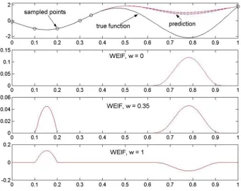
Let us consider the one-variable function shown at the top of Figure 1. We assume that it has been sampled in the six points indicated on the plot as circles and an RBF approximation has been constructed. The predictor is also shown in the top section of the figure. The dashed lines either side of the predictor represent the predictor plus and minus one standard error. On the left-hand side of the plot this is very small, as the density of the sam-ple is much larger there – the error is only visible in the fairly large gap between the fifth and sixth points.

The uneven distribution of these points may seem slightly unrealistic in a DoE context. Nevertheless, such situations regularly occur in higher dimen-sions and/or after a few infill points have been added to the database.

The section of the figure placed below this plot shows the weighted expected improvement with weightingw=0. Based on the above discussion,

we would expect the WEIF measure to give the search a fully global bias. This is indeed the case, as the sole maximum of the criterion is in the sparsely sampled region, where the uncertainty about whether the function value is better than the current best point is high. Note that the “good-ness” of the prediction, i.e., the value of the predictor, is not influencing the optimization based on the WEIF with w=0: the weighted criterion guides us to near the middle of the unsampled region, in spite of the predicted objective being rather poor here.

As we increase w, i.e., we give the search a more local flavor, another peak starts to emerge in WEIF on the left-hand side where the predictor indicates good function values (although the uncertainty is very low here). When we reach w=0.35 (see the third section of Figure 1) the impor-tance of exploration and exploitation becomes approximately equal (the two peaks are of equal height).

The bottom section of Figure 1 shows the WEIF landscape for w=1. Clearly, maximizing this surface will yield a single optimum, which will be in the lowest predicted objective function value point. Wherever the predic-tion is worse than the current best point, the WEIF will be negative (due to the ymin− ˆy factor in the first term of Equation (13)).

A final aspect of our generic two-stage optimization strategy, which we need to discuss before looking at more complex examples, is the way in which we handle constraints imposed on the objective function – we do this in the following section.

4. Dealing with constrained objectives

Constrained expensive optimization problems come in two flavors. The objective is either constrained by a function that can be evaluated at neg-ligible cost (this usually means that it can be calculated using some closed form expression) and thus it is known exactly throughout its domain (we present an engineering design example for this in Section 5) or by another computationally expensive function, in which case this, just like the objec-tive, needs to be approximated.

might perform on constrained problems.2 We simply set the criterion to zero wherever the approximate or exact constraints are violated

WEIF(x)= ⎧ ⎪ ⎪ ⎪ ⎪ ⎪ ⎪ ⎪ ⎪ ⎪ ⎨ ⎪ ⎪ ⎪ ⎪ ⎪ ⎪ ⎪ ⎪ ⎪ ⎩

w(ymin− ˆy) _y

min− ˆy

s

+(1−w)sψymin− ˆy

s

if s >0 and the (approximate or exact) constraints are satisfied,

0

if s=0 or if the (approximate or exact) constraints are violated.

(14)

Here ymin should be taken as the minimum feasible response (assuming, of

course, that the initial sample contains at least one feasible point3), where feasibility is assessed on the basis of the exactly known or the approxi-mate constraint value in each sampled point, depending on the cost of the constraint.

We are now ready to proceed to examine the effects of local/global bias of the WEIF, in conjunction with that of starting from different initial samples, on the performance of a two-stage optimization algorithm. We use artificial test functions first, followed by two “real-life” engineering applications.

5. Empirical results

5.1. artificial test functions

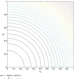
For the purposes of this study we have selected three test functions. In order of increasing complexity they are the Sphere, a modified version of Rosen-brock’s “banana” function and the highly multimodal Ackley function (Ack-ley, 1987). Figures 2–4 represent these functions in two dimensions (please refer to the captions for details on their definition) – we have looked at the performance of the WEIF-based optimizer on the 5-variable versions and in one case (Ackley’s) on the 10-dimensional landscape as well.

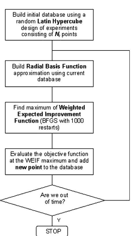
The optimization algorithm we have used to perform this empirical study is shown in Figure 5. We start by generating an initial database of points and we evaluate their objective function values. A random Latin Hypercube

2_{Difficulties could arise here when the optimum is on a constraint boundary. There is a rich}

literature on how to tackle this problem within various optimization algorithms – the interested reader may consult, for example, the seminal work of Fiacco and McCormick (1968).

3_{If the initial sample does not contain a feasible point, one can start by applying the}

Figure 2. Sphere function.

fS= N

i=1

x2

i, xi∈[0,1].

experimental design is used to build these initial designs. In order to alle-viate the effects of any bias due to some of these initial points falling, by sheer luck, close to the global optima of the studied functions, each result is averaged over 30 runs (except where otherwise stated).

Figure 3. Modified Rosenbrock function, normalized to [0,1] (ak-dimensional sinewave has been added to the Rosenbrock function to increase its modality).

fMR= k−1 i=1

100(xi+1−x2i)2+(1−xi)2+ k

i=1

75 sin(5(1₋xi)), xi∈[₋2.048,2.048].

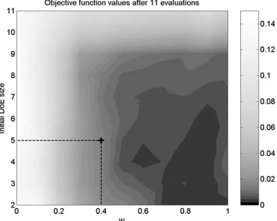
For the visualization of the results we have opted for a greyscale snap-shot map format. The density of a particular region of the plot represents the (averaged) objective function value reached by an optimizer started from an initial Latin Hypercube sample of the size shown on the vertical axis, using the WEIF weighting indicated by the horizontal axis. Looking back at the discussion of the relationship between the scope of the search and the WEIF weighting, the closer we are to the left edge of the plot the more global the search is – conversely, moving to the right gradually reduces the scope of the WEIF criterion.

Figure 4. Ackley’s path function, normalized to [0,1].

fACK= −aexp

−b

1 n

k

i=1

x2 i

−exp

1 n

k

i=1

cos(cxi)

+a+exp(1), xi∈[₋2.048,2.048].

selected using the WEIF criterion with a weighting of 0.4 (the abscissa of the point). This, referring again to the analysis in Section 2, relates to an optimization with a slightly broader scope (more global) than that of the conventional expected improvement criterion (w=0.5).

Due to the high computational expense of generating these plots, in most cases it was impractical to run the tests for every possible initial DoE size and for a very large number of different weightings – the density maps are therefore regressors through the actual data points. For each initial DoE size the optimizer has been run with 11 different weightings, covering the range between 0 and 1 with increments of 0.1. Each set of runs was stopped after some of the runs achieved an optimal (or very close to the optimum) solution – in the case of Figure 6, for example, after 11 evalua-tions of the objective function.

Figure 5. Optimization algorithm based on the WEIF infill sample selection criterion.

comparatively little room for variation in the crucial “fine-tuning” phase (with the exception of runs with very bad parameter choices, which make very slow progress throughout the search process). Therefore, in order to distinguish between the various areas belonging to “relatively good” initial DoE sizes and weightings, the density map is based on a logarithmic scale (as shown by the density bar adjacent to each figure).

Figure 6. Log-scale colourmap of objective function values reached by the optimizer after 11 evaluations of the 5-variable Sphere function, using various WEIF weightings (horizontal axis) and initial samples of various sizes (vertical axis). The darker areas correspond to better objec-tive values.

initial DoE sizes the problem is solved after 11 evaluations – as indicated by the large black area in the lower right-hand corner of the plot. As expected, a fairly localized search (with weightings ranging from 0.7 to 1) gives the best results.

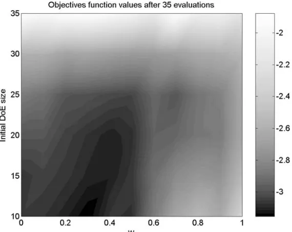
A different landscape, the considerably multimodal Modified Rosenbrock function, yields a dramatically different plot (see Figure 7). On this occa-sion the black area emerging after 35 evaluations of the objective func-tion is centered around a weighting of 0.3 for small initial sample sizes and leans slightly towards w=0.4 as we move up into the zone of 15–20 point initial DoEs.

Figure 7. Log-scale colourmap of objective function values reached by the optimizer after 35 evaluations of the 5-variable Modified Rosenbrock function, using various WEIF weightings (horizontal axis) and initial samples of various sizes (vertical axis). The darker areas correspond to better objective values.

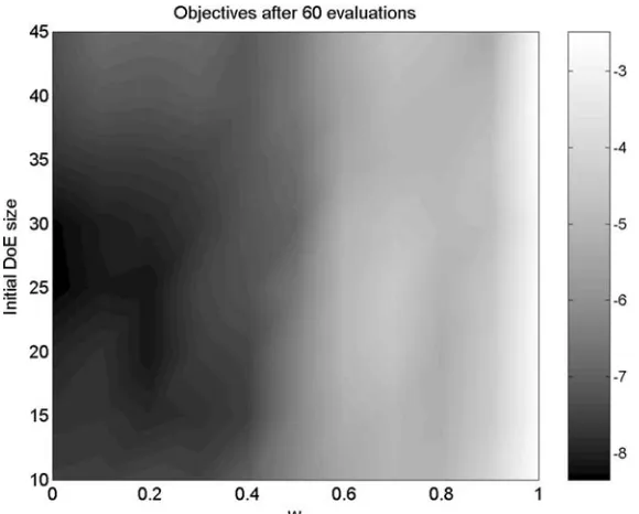
a snapshot of objective values after 60 evaluations of the same function (Ackley), this time in 10 dimensions.

We note here that this last plot is only averaged over 10 runs, due to its high computational expense. The optimizer was run for 8 different initial DoE sizes (10, . . . ,45), in each case for 11 different weightings (0, . . . ,1, increments of 0.1). With an initial DoE size of 10 the RBF model needs to be retrained and rebuilt 50 times (to reach the total objective function evaluation count of 60), starting from 15 points requires 45 constructions of the model, etc. This amounts to 50+45+ · · · +15=260 runs of the training procedure for each WEIF weighting factor, that is 260×11=2860 across the entire range. Averaging over 10 runs thus gives a total figure of 28600 models that need to be trained. With one such procedure taking, on average, around 60 s on a PIII processor for a 10-variable problem, the required CPU time works out to 429 h for this plot alone.

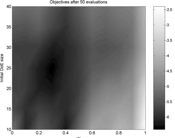
Figure 8. Log-scale colourmap of objective function values reached by the optimizer after 50 evaluations of the 5-variable Ackley function, using various WEIF weightings (horizontal axis) and initial samples of various sizes (vertical axis). The darker areas correspond to better objec-tive values.

size of the initial sample is too large we are likely to waste points by placing them simply in a space-filling manner, instead of using information gained from the objective values of previous points (via some approxima-tion model-based criterion). The opposite problem becomes evident when looking at either of the two Ackley plots (Figures 8 and 9). A very small initial DoE sample (10–15 points) often renders any approximation-based criterion almost entirely meaningless – as the contrast between this region and the much darker one above it (20–30 initial points) indicates, more can be gained by at least ensuring that these points fill the space uniformly, without using the objective values of the other points to decide on their location.

Figure 9. Log-scale colourmap of objective function values reached by the optimizer after 60 evaluations of the 10-variable Ackley function, using various WEIF weightings (horizontal axis) and initial samples of various sizes (vertical axis). The darker areas correspond to better objec-tive values.

budget (one obvious exception to this rule is where such a choice would lead to a number of calculations that did not efficiently fill the available computing facilities – in such cases using more points would probably be more sensible).

a Latin Hypercube design optimized on some space-filling criterion (e.g., a maximum–minimum distance criterion). The choice of which weighting to use for the selection of the remaining 65% of the points ultimately comes down to the judgment and experience of the analyst. Relatively few real-life problems generate landscapes as highly multimodal as the Ackley function. Nevertheless, if this appears to be the case (based on previous experience on similar problems), one is well advised to keep the scope of the search fairly global (w∈[0,0.3]). For problems where one can be reasonably confident of the accuracy of the initial prediction, values in the range [0.2,0.5] are recom-mended, depending on the modality of the function. Finally, w=0.5 should only be exceeded when one is confident that the landscape is of low modality. Many real-life engineering problems exhibit simple, unimodal behavior – in these cases running the WEIF-based optimizer with a weighting of around 0.9 can be expected to give good results. In the following section we discuss an application of this nature.

5.2. a “real-life” unimodal problem: geometric optimization of a spoked structure

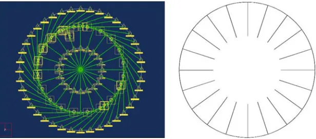
In this case study we consider the optimization of the spoked structure shown in Figure 10 (left). This model is made up entirely of beam ele-ments whose thickness can be altered in a variety of ways. The part of the structure being optimized is shown on the right-hand side of the figure. Six design parameters define the geometry, five of which describe the ring cross section while the sixth describes the spoke sections. The rest of the model simply enforces suitable boundary conditions. Our industrial collaborators provided realistic loadings to place on the structure.

The goal here is to minimize the maximum von Mises stress (com-puted using the ProMecanicaTM _{package) within the structure such that the}

Figure 11. Two-dimensional section through the objective function of the structural testcase. The feasible region is delimited by the linear mass constraint.

weight does not exceed a predefined value. Calculating the stress involves solving the finite element problem at a cost of about 100 s of CPU time, the weight is simply the result of evaluating an exact linear model (at negligible cost) and thus can be calculated for each sampled point without incurring significant computational overheads. The WEIF updates are performed in the manner described in Section 4.

To check our conjecture that this problem is likely to generate a sim-ple, unimodal objective we have computed a two-variable slice through the six-dimensional landscape – this is shown in Figure 11. The contour plot confirms the conjecture, as it shows a single minimum on the constraint boundary. Of course, in general we do not have the luxury of generating such plots (if we had we would not need an optimizer) – here we needed this insight to underpin our subsequent conclusions with respect to the choice of the WEIF weighting.

Figure 12. Log-scale colormap of objective function values reached by the optimizer after 40 evaluations of the stress function (spoke structure).

5.3. a case of higher modality: vibration optimization of a two-dimensional structure

Our final study concerns optimization of the frequency response of a two-dimensional structure of the sort that may be found in girder bridges, tower cranes, satellite booms, etc. (Renton, 1999). It consists of 40 individual Euler–Bernoulli beams connected at 20 joints. Each of the 40 beams has the same properties per unit length.

Initially the boom was designed and analyzed for a regular geometry, where each beam was either 1 m or 1.414 m in length, as shown in the top section of Figure 13. The joints at points (0,0) and (0,1) are fixed, i.e., they are fully restrained in all degrees of freedom, all other joints are free to move. The structure is excited by a point transverse force applied halfway between points (0,0) and (1,0) (as indicated by the arrow on Fig-ure 13). The vibrational energy level was found for the right-hand end ver-tical beam using matrix receptance methods based on the Green functions of the individual beam elements, which are set up to calculate the forces and velocities at the joints (Keane, 1995). This approach allows for a quick calculation of the energy flows around the structure. The results of the analysis have been validated experimentally (Keane and Bright, 1996).

The objective was the minimization of the frequency averaged response of the beam in the range 150–250 Hz.

having sides of 0.5 m, centered on the initial points (see Figure 13), thus generating a four-dimensional optimization problem. The rest of the struc-ture remained unchanged.

Again, to make the correlation between the optimum expected improve-ment weighting and the complexity of the landscape clearer, we have pro-duced a two-variable slice through the design space. Figure 14 shows a contour plot of the energy level function, as measured on the right-hand end vertical beam.

As expected, this low modality (but no longer unimodal) problem dic-tates a weighting higher than 0.5, but lower than 0.8 (see Figure 15). In fact the dark region of the corresponding weighting-DoE size map is cen-tered around w=0.7.

As far as the optimum population size is concerned, 35% (10 points) is still a safe choice, although in this case the performance is just as good if one starts with a very small initial DoE.

6. A variable bias update strategy

We have seen in Section 5 how a rough knowledge of the complexity of the objective function can prove to be a valuable aid in choosing the right global-local bias (i.e., the weighting w) for the global optimization process. However, it is not uncommon in engineering design practice that very lit-tle is known about the nature of the objective, in which case there is no

Figure 14. Two-dimensional section through the vibrational energy level function of the truss testcase. (x1 is the x-coordinate of joint, x2 is the y-coordinate of the same joint).

obvious alternative means of selecting the best bias without incurring sig-nificant computational expense in doing so.

For such situations Gutmann (2001) suggests cycling through the avail-able range of global-local balances as the search progresses. He picks an infill point using a highly global setting of his criterion, the following five points to be sampled being selected by gradually shifting the balance towards exploitation. This six-step pattern is then repeated for the rest of the search. Since the same bias variation is used for all functions, the need for choosing the bias-related runtime parameter(s) is eliminated.

Here, we suggest implementing this heuristic by cycling through the pattern w= {0.1,0.3,0.5,0.7,0.9}. Thus, like Gutmann, we start from an exploratory weighting and we move towards exploitation – this pulsating search scope pattern is then repeated until we run out of time or some other stopping criterion is met.

Figure 15. Log-scale colormap of objective values reached by the optimizer after 30 evaluations of the vibrational energy level function (two-dimensional truss).

Table I. Main features of the Dixon–Szeg ¨o test problems

Test function Dimensionality Local minima Global minima

Branin 2 3 3

Goldstein-Price 2 4 1

Hartman 3 3 4 1

Hartman 6 6 4 1

Shekel 5 4 5 1

Shekel 7 4 7 1

Shekel 10 4 10 1

compare our performance figures with. Amongst others, Jones et al. (1998), Bj ¨orkman and Holstr ¨om (1999) and Gutmann (2001) run their techniques on most of the Dixon–Szeg ¨o functions – we use the same test problems, the most important features of which are summarized in Table I.

Table II. Comparative optimizer performance table showing the number of evaluations required by the various optimizers to get to within 1% of the global optima of the Dixon-Szeg ¨o test functions (the error of convergence is defined asE=100(fmin−fglobal)/|fglobal|, wherefmin is the current best

objective function value and fglobal is the global optimum of the function).

Evaluation count whenE <1%

Test function WEIF cyclic Gutmann DIRECT EGO

Branin 34 44 63 28

Goldstein-Price 32 63 101 32

Hartman 3 28 25 83 35

Hartman 6 33 112 213 121

Best of 10 runs

Shekel 5 43 76 103 –

Shekel 7 84 76 97 –

Shekel 10 63 51 97 –

The WEIF cyclic bias variation algorithm results are averages over 10 runs, except those for the Shekel functions, which are referring to the best of 10 runs. The runs were started from an initial set of 10 training points, arranged in a latin hypercube experimental design.

been started from different, randomly generated latin hypercube experimen-tal designs. As before, the purpose of this experimenexperimen-tal setup was to eliminate the effect of chance, i.e., the effect of distorted performance figures caused by one or more points of the initial design landing near the global basin.

As the table shows, the WEIF-based cyclic bias variation algorithm works well on most of the test functions that we have experimented with here. The Shekel functions might be considered to be an exception to this – here the objective values after 150 evaluations for versions 5, 7 and 10 were still short of the global optima (by 13.88%, 20.09% and 11.26%, respectively). In each case, however, there was at least one run that did reach the 1% threshold within this budget – the performance figures for the best of these are shown in the table. This indicates that, like many other approximation-based algorithms, a search based on the WEIF update scheme may be inefficient on “needle in a haystack” type problems (such as Shekel’s “foxholes”) – thankfully, such problems are relatively rare in engi-neering design optimization. We also note here that the comparative table presented here should be considered in the light of the fact that the results for Gutmann’s algorithm and EGO do not take into account the variability of the performance resulting from the variability in the choice of the initial sampled points (this can make a particularly large difference when the rel-ative area of the basins of attraction is very small, as in the case of the Shekel function family).

7. Conclusions and future work

introduction of a criterion that allows easy control of the scope of the search when selecting infill sample points. We have looked at the effects of biasing the infill selection via this criterion, either towards global explora-tion or towards exploitaexplora-tion of promising areas, through a set of empirical tests.

The two aspects we were most interested in were the selection of an appropriate weighting factor (which controls the scope of the criterion and thus the scope of the search) and the selection of the size of the initial DoE set of sampled designs. One of the most important conclusions of these experiments was the relatively high importance of these factors from the point of view of search efficiency, as highlighted by the sharp contrasts seen on some of the optimizer performance maps. However, these maps also indicate that there is some safety margin in choosing the two param-eters.

Naturally, there is always room for further refinement and verification of these guidelines. The set of objective functions examined here is fairly limited and the results relevant to the choice of the initial sample size are based on a single computational budget in each case. Other types of approximation models could also be considered, including gradient-enhanced global approximations (where the objective function gradients can be obtained cheaply). Although the computational expense of build-ing such maps can be relatively high, they are worth the effort if one is often confronted with optimization problems belonging to the same class and therefore such fine-tuning of the optimizer can be justified.

For those cases where no information is available on the complexity of the objective function, we have assessed the performance of a variable global–local bias scheme. The results obtained on a set of test functions (compared with other approximation-based techniques) are encouraging and indicate that the weighted expected improvement criterion can play a significant role even when we have no prior knowledge of the problem under scrutiny. We note here that future work in this area could include an extension of the variable bias scheme for parallel architectures, where each set of parallel updates could contain points selected with different values of the weighting (covering a range of balances from global to local).

Acknowledgements

References

Ackley, D.H. (1987), A Connectionist Machine for Genetic Hillclimbing, Kluwer Academic Publishers, Boston.

Audet, C., Dennis, J.E., Moore, D.W., Booker, A. and Frank P.D. (2000), A surro-gate-model-based method for constrained optimization, In: 8th Proceedings of the AIAA/NASA/USAF/ISSMO Symposium on Multidisciplinary Analysis and Optimization, Long Beach, CA.

Bj ¨orkman, M. and Holstr ¨om, K. (1999), Global optimization using the DIRECT algorithm in Matlab,Advanced Modeling and Optimization 1(2), 17–28.

Dixon, L.C.W. and Szeg ¨o, G. (1978), The Global optimization problem: an introduction, In Dixon, L.C.W. and Szego, G. (EDS.), Towards Global Optimization, North Holland, Amsterdam, 2, pp. 1–15.

Fiacco, A.V. and McCormick, G.P. (1968),Nonlinear Programming: Sequential Unconstrained Minimization Techniques, Wiley, New York.

Gibbs, M.N. (1997), Bayesian Gaussian Processes for Regression and Classification, PhD thesis, University of Cambridge.

Gutmann, H.M. (2001), A radial basis function method for global optimization,Journal of Global Optimization19(3), 201–227.

Jones, D.R. (2001), A taxonomy of global optimization methods based on response surfaces, Journal of Global Optimization21, 345–383.

Jones, D.R., Schonlau, M., and Welch, W.J. (1998), Efficient global optimization of expen-sive black-box functions, Journal of Global Optimization13, 455–492.

Keane, A.J. (1995), Passive vibration control via unusual geometries: the application of genetic algorithm optimization to structural design, Journal of Sound and Vibrations 185(3), 441–453.

Keane, A.J. and Bright, A.P. (1996), Passive vibration control via unusual geometries: exper-iments on model aerospace structures, Journal of Sound and Vibrations190(4), 713–719. Mackay, M.D., Beckman, R.J. and Conover, W.J. (1979) A comparison of three methods for

selecting values of input variables in the analysis of output from a computer code, Tech-nometrics21, 239–245.

Mockus, J., Tiesis, V. and Zilinskas, A. (1978), The application of bayesian methods for seek-ing the extremum,Towards Global Optimization, North Holland, Amsterdam, 2, 117–129. Montgomery, D. (2000),Design and Analysis of Experiments, 5th edn, Wiley, New York. Renton, J.D. (1999),Elastic Beams and Frames, Camford Books.

Sasena, M.J., Papalambros, P. and Goovaerts, P. (2002), Exploration of metamodeling sam-pling criteria for constrained global optimization,Engineering Optimization 34, 263–278. Schonlau, M. (1997),Computer Experiments and Global Optimization, PhD thesis, University

of Waterloo, Canada.

S ´obester, A., Leary, S.J. and Keane, A.J. (2004), A parallel updating scheme for approxi-mating and optimizing high fidelity computer simulations,Structural and Multidisciplinary Optimization 27, 371–383.

Sobol, I.M. (1979), On the systematic search in a hypercube, SIAM Journal of Numerical Analysis 16, 790–793.

Trosset, M.W. and Torczon V. (1997), Numerical optimization using computer experiments, technical report TR-97-38, ICASE, NASA Langley Research Center, Hampton, Virginia. Watson, A.G. and Barnes, R.J. (1995), Infill sampling criteria to locate extremes,