M estimator and D optimality model construction using orthogonal forward regression

M-Estimator and D-Optimality Model Construction

Using Orthogonal Forward Regression

Xia Hong

, Senior Member, IEEE

and

Sheng Chen

, Senior Member, IEEE

Abstract—This correspondence introduces a new orthogonal forward regression (OFR) model identification algorithm using D-optimality for model structure selection and is based on an M-estimators of parameter estimates. M-estimator is a classical robust parameter estimation tech-nique to tackle bad data conditions such as outliers. Computationally, The M-estimator can be derived using an iterative reweighted least squares (IRLS) algorithm. D-optimality is a model structure robustness criterion in experimental design to tackle ill-conditioning in model structure. The orthogonal forward regression (OFR), often based on the modified Gram–Schmidt procedure, is an efficient method incorporating structure selection and parameter estimation simultaneously. The basic idea of the proposed approach is to incorporate an IRLS inner loop into the modified Gram–Schmidt procedure. In this manner, the OFR algorithm for parsimonious model structure determination is extended to bad data conditions with improved performance via the derivation of parameter M-estimators with inherent robustness to outliers. Numerical examples are included to demonstrate the effectiveness of the proposed algorithm.

Index Terms—Forward regression, Gram–Schmidt, identification, M-es-timator, model structure selection.

I. INTRODUCTION

Various neural networks such as radial basis function (RBF)

net-works can be expressed as a linear-in-the-parameters model structure

where the system output is a linear combination of nonlinear basis

functions. Provided that there is a separate mechanism for determining

centers/widths of these basis functions, the basis weights/parameters

can be trained using linear optimization techniques. The architecture

or topology of the class of linear-in-the-parameters modeling networks

enables them to be readily assessed in terms of their modeling

capa-bility, structure, learning, construction, and numeric stacapa-bility, since the

results of quadratic optimization and linear algebra are directly

appli-cable. Moreover, by applying linear regression statistical techniques to

the identification of this type of neural networks, it is possible to model

the observational data in a statically optimal sense to achieve improved

performance for a wide range of applications/tasks in the field of signal

processing, dynamical system modeling, and control.

The general method of M–estimation [1] is well established in

order to tackle outliers in observational data. As a generalization of

maximum-likelihood estimation method for data with outliers, the

M-estimator uses some cost functions which increase less rapidly than

that of least squares estimators as the residual departs from zero, so

the parameters estimator is more robust to outliers. Computationally,

M-estimator can be derived using an iterative reweighted least squares

(IRLS) algorithm. M-estimation has been applied successfully to

time series prediction, image processing and pattern recognition

[2]–[4]. Two major aspects of system identification are model

struc-ture determination and parameter estimation. While M-estimator is

Manuscript received March 11, 2004; revised June 14, 2004. This work was supported by the EPSRC UK. This paper was recommended by Associate Editor P. De Wilde..

X. Hong is with the Department of Cybernetics, University of Reading, RG6 6AY Reading, U.K.

S. Chen is with the School of Electronics, University of Southampton, SO17 1BJ Southhampton, U.K.

Digital Object Identifier 10.1109/TSMCB.2004.839910

concerned with parameter robustness, conventional optimum

exper-imental designs are concerned with model structure robustness [5].

In optimum experimental design, model adequacy is evaluated by

statistical measures of goodness via experimental design criteria, e.g.

A- and D-optimality. By quantitatively measuring the model adequacy

as function of the eigenvalues of the design matrix, design efficiency

and experimental effort of designs can be optimized.

The orthogonal forward regression (OFR) is an efficient algorithm

to determine a parsimonious model structure [6]. Driven by

require-ments for improved model generalization, a few variants of OFR have

been introduced in order to tackle ill-conditioning problem that may be

associated with least squares parameter estimates [7]–[11]. Recently,

variants of the forward OFR algorithms have been introduced by

mod-ifying the selective criteria to include A- and D-optimality in forward

regression [12], [13] to form hybrid approaches applicable to neural

networks modeling. Although these methods do not generally need the

assumption of a normal error distribution, the parameter estimator may

not be statistically optimal if the data exhibit bad conditions such as

outliers.

Alternatively there exists a vast amount of work on sparse modeling

including the well-known support vector machine (SVM) [14], which

is often used in classification tasks [15] and can also be used in sparse

regression modeling [16]. SVM is regarded as a robust modeling

ap-proach and based on a structural risk minimization (SRM) principle,

that is to minimize an estimate of the upper bound of model

general-ization. The model sparsity and robustness of SVM can be achieved

by incorporating an

"

-insensitive function in the loss function, as

pro-posed by Vapnik [14]. The

"

-insensitive function and Huber loss

func-tion used in M-estimator shares a similarity of using

l

1

norm (see

Sec-tion II-A). Because the implementaSec-tion of SVM sparse modeling with

the

"

-insensitive function is solved via constrained quadratic

program-ming (QP), it is computationally expensive. It has been shown that OFR

algorithm can be combined with SVM to improve model sparseness

[16].

This paper presents a new model identification algorithm that

com-bines the M-estimator with forward regression. Based on the modified

Gram–Schmidt procedure for OFR, the proposed algorithm

incorpo-rates an IRLS inner loop into the modified Gram–Schmidt procedure

to derive the M-estimator of model parameters. In combination with

D-optimality for model structure selection, the proposed algorithm

si-multaneously derive robust model structure and parameter estimates

for bad data conditions.

The paper is organized as follows. Section II initially introduces

methodologies relevant to the proposed algorithm, including general

nonlinear regression modeling based on OFR algorithm with

D-opti-mality and the concept of the M-estimator. Section III introduces the

model identification algorithm using forward regression with

M-esti-mation. Numerical examples are used to demonstrate the efficacy of

the algorithm in Section IV and conclusions are given in Section V.

II. PRELIMINARIES

A linear regression model (RBF neural network, B-spline

neuro-fuzzy network) can be formulated as [17], [18]

y(t) =

M

k=1

p

k

(x(t))

k

+ (t)

(1)

where

t = 1; 2; 1 1 1 ; N

, and

N

is the size of the estimation data set.

y(t)

is system output variable,

x(t) = [x

₁

(t); 1 1 1 ; x

_n

(t)]

T

is system

input vector with an assumed known dimension of

n

.

p

k

()

is a known

nonlinear basis function, such as RBF, or B-spline fuzzy membership

functions.

(t)

is an uncorrelated model residual sequence with zero

mean and variance of

2

.

_k

is model parameter, and

M

is the number

of regressors.

Equation (1) can be written in the matrix form as

y = P2

2 + 4

2

(2)

where

y = [y(1); 1 1 1 ; y(N)]

T

is the output vector.

2

2

2 =

[

1

; 1 1 1 ;

M

]

T

is parameter vector,

4 = [(1); 1 1 1 ; (N)]

T

is

the residual vector, and

P

is the regression matrix

P =

p

1

(1)

p

2

(1)

1 1 1 p

k

(1) 1 1 1

p

M

(1)

p

1

(2)

p

2

(2)

1 1 1 p

k

(2) 1 1 1

p

M

(2)

p

1

(N) p

2

(N) 1 1 1 p

k

(N) 1 1 1 p

M

(N)

with

p

_k

(t) = p

_k

(x(t))

. Denote the column vectors in

P

as

p

_k

=

[p

k

(1); 1 1 1 ; p

k

(N)]

T

,

k = 1; 1 1 1 ; M

. An orthogonal decomposition

of

P

is

P = WA

(3)

where

A = f

ij

g

is an

M 2 M

unit upper triangular matrix and

W

is an

N 2 M

matrix with orthogonal columns that satisfy

W

T

_{W =}

_diag

_f

1

; 1 1 1 ;

M

g

(4)

with

k

= w

kT

w

k

; k = 1; 1 1 1 ; M

(5)

so that (2) can be expressed as

y = (PA

01

_{)(A2) + 4 = W0 + 4}

₍₆₎

where

0 = [

₁

; 1 1 1 ;

_M

]

T

is an auxiliary vector. The above

orthog-onal decomposition can be realized by the modified Gram–Schmidt

algorithm [6], in which least squares parameter estimates are usually

used. Based on the modified Gram–Schmidt algorithm, a few variants

of forward OLS algorithms have been introduced to improve model

generalization capability based on the concepts from Bayesian

regular-ization/basis pursuit [9], experimental design and leave-one-out (LOO)

score, respectively, [10], [11]. Although these methods do not generally

need normality error distribution assumption, the parameter estimator

may not be statistically optimal if the data exhibit bad conditions such

as outliers, or are heavy tailed. The general method of tackling this

problem is well established as M-estimation [1], which is a

generaliza-tion of maximum-likelihood estimageneraliza-tion method for data with outliers.

The M-estimator [1] is described in the following section.

A. M-Estimators

The M-estimators have been well studied [1]. Considering the linear

regression model given by (1), the M-estimator minimizes the cost

function

V

M

=

N

t=1

((t))

(7)

where the function

((t))

is some predetermined non-negative

func-tionals for different types of estimators, e.g., for least squares

((t)) =

L

((t)) =

2

(t)

. Typically,

((t))

is an even function and

nonde-creasing with respect to the absolute value of

(t)

. The problem of least

squares estimator is that

V

M

will be influenced by any outlier typified

by a large absolute value

(t)

. The general M-estimator can tolerate

undetected outliers by assigning a smaller weight to observations with

residuals with large absolute values, so the parameter estimates are less

vulnerable to unusual data. The most common types of M-estimators

are the

Huber

estimator given by [1]

H

() =

1

2

2

;

for

jj

jj 0

1

2

2

;

for

jj >

(8)

or the Turkey

bisquare

estimator, given by

B

() =

6

1 0 1 0

2 3

_;

for

jj

1

6

2

for

jj >

(9)

where the parameter

is called a tuning constant, e.g. it is common to

choose

= 1:345

for the

Huber

estimator and

= 4:685

for the

Turkey

bisquare

estimator.

1

The M-estimator can be derived by setting

@V

M

@2

_{2= ^2}

= 0

(10)

to yield

@V

M

@2

= P

T

= 0

(11)

where

0

is zero vector.

= @V

M

@(1)

; . . . ; @V

@(N)

M T

= [ ((1)) ; . . . ; ((N))]

T

(12)

where

()

is the derivative of

()

with respect to

. Define the weight

function

!(t) = ((t))

_(t)

;

for

t = 1; . . . ; N:

(13)

Equation (11) can be written as

P

T

_{4 = 0}

₍₁₄₎

where

=

diag

f!(1); !(2); . . . !(N)g

, whose solution is given as

the weighted least squares

^

2

M

= fP

T

Pg

01

P

T

y:

(15)

Because

!(t)

s are primarily unknown, an iteratively reweighted least

square (IRLS) is required. The M-estimator IRLS procedure is as

fol-lows:

Denote

m

as the iteration step. Initially set

m = 1

,

(1)

= I

(i.e.

least squares) to derive an initial model residuals

(1)

(t)

, then for

m =

2; . . . ; m

w

!

(m)

_{(t) =}

(m01)

_(t)

(m01)

_(t)

;

for

t = 1; . . . ; N:

(16)

From (8) and (9), the weight functions of

Huber

and the Turkey

bisquare

estimator can be explicitly given by

!

(m) H

(t) =

1;

for

(m01)

(t)

j

(t)

j ;

for

(m01)

(t) >

(17)

1_{The theoretic foundation of choosing these values is due to [1] in that these}

and

!

(m) B

(t) =

1 0

(t) 2 2

;

for

(m01)

(t)

0;

for

(m01)

(t) >

(18)

respectively. Let

(m)

=

diag

f!

(m)

(1); !

(m)

(2); . . . !

(m)

(N)g

;

then

^

2

(m)_M

= P

T

(m)

_P

01

_P

T

(m)

_y

₍₁₉₎

4

(m)

_{= y 0 P ^}

₂

(m)

M

(20)

where

4

(m)

= [

(m)

(1); 1 1 1 ;

(m)

(N)]

T

are ready for next iteration

step. The above procedure iterates until the parameter estimator

2

^

M

converges at

m = m

_w

.

^

2

M

= P

T

(m )

P

01

P

T

(m )

_y:

₍₂₁₎

The asymptotic covariance matrix of

2

^

M

is given by [1]

var

[ ^

2

M

] = E(

2

₎

E

2 d d

(P

T

_P)

01

_:

(22)

From (22), it is seen that the efficiency of the M–estimator depends

on the full rank of the

(P

T

P)

01

. However this usually may not be

true for an oversized

P

, unless there is some robustness measure in

place to select a parsimonious model structure. Robust model structure

selection can be achieved via experimental design criteria that selects

P

T

k

P

k

, where

P

k

is a subset of

P

, if

P

T

P

is ill-conditioned. The

basic OFR model structure detection algorithm using D-optimality [13]

is initially given below, which will be incorporated in the proposed

algorithm of Section III.

B. Model Structure Selection by D-Optimality

A significant advantage due to orthogonalization is that the

contribution of model regressors to the model can be

evalu-ated. The OFR estimator involves selecting a set of

n

variables

p

k

= [p

k

(1); 1 1 1 ; p

k

(N)]

T

,

k = 1; 1 1 1 ; n

, from

M

regressors

to form a set of orthogonal basis

w

k

,

k = 1; 1 1 1 ; n

, in a forward

regression manner. As the orthogonality property

w

T_i

w

_j

= 0

for

i 6= j

holds, if (6) is multiplied by itself and then the time average is

taken, the following equation is easily derived

1

N

y

T

y = 1

N

M

k=1

2

k

w

Tk

w

k

+ 1

_N

4

T

4:

(23)

The most relevant

n

regressors can be forward selected

ac-cording to the value of an error reduction ratio

[

ERR

]

_k

(defined

as

_k2

w

T_k

w

_k

=y

T

y

, see [6]). At the

k

th selection, a candidate regressor

is selected as the

k

th basis of the subset if it produces the largest value

of

[

ERR

]

_k

from the remaining

(M 0 k + 1)

candidates. This

proce-dure can automatically select a subset of

n

regressors to construct a

parsimonious model. Equivalently, this procedure can be expressed as

J

(k)

_{= J}

(k01)

_{0 1}

N

k2

k

(24)

where

J

(0)

= y

T

y

. At the

k

th forward regression stage, a candidate

regressor is selected as the

k

th regressor if it produces the smallest

J

(k)

.

Equation (24) can be modified to form an alternative model selective

criterion to enhance model robustness. The D-optimality criterion [5]

maximizes the determinant of the design matrix defined as

W

T_k

W

k

max J

D

= det W

Tk

W

k

=

n

k=1

k

(25)

where

W

k

2 <

N2n

denotes the resultant regression matrix,

con-sisting of

n

regressors selected from

M

regressors in

W

. It can be

easily verified that the selection of a subset of

W

k

from

W

is

equiv-alent to the selection of the a subset of

n

regressors from

P

[13].

In order to include D-optimality as a model selective criterion for

im-proved model robustness, construct an augmented cost function as

J = 1

_N

4

T

_{4 + log}

1

J

D

= 1

_N

y

T

_{y 0}

n k=1

2

k

k

+

n

k=1

log 1

k

(26)

where

is a positive small number. Note that this composite cost

func-tion simultaneously minimizes (24) and maximizes (25) [13]. Equafunc-tion

(26) can be directly incorporated into the OFR algorithm to select the

most relevant

k

th regressor at the

k

th forward regression stage, via

J

(k)

= J

(k01)

0 1

_N

k2

k

+ log 1

k

:

(27)

At the

k

th forward regression stage, a candidate regressor is selected as

the

k

th regressor if it produces the smallest

J

(k)

and further reduction

in

J

(k01)

. Because

log(1=J

D

)

is an increasing function if

k

< 1

,

which is true for some

k > K

, the selection procedure will terminate

if

J

(k)

J

(k01)

at the derived model size

n

if an proper

is set.

This is significant because this means that the proposed approach can

detect a parsimonious model size in an automatic manner.

A method of orthgonalization as required in above procedure is the

modified Gram–Schmidt procedure [6]. In [13],

_k

are derived as least

squares estimates. In the following, we propose a new algorithm as how

to incorporate D-optimality model structure selection with M-estimator

(Section II-A). The basic idea is to extend the modified Gram–Schmidt

algorithm to include, at every forward regression step, an IRLS

proce-dure inner loop that derives the M-estimator for the auxiliary vector

0

.

III. MODEL

IDENTIFICATION

ALGORITHM

USING

FORWARD

REGRESSION

WITH

M-ESTIMATION

Starting from

k = 1

, the columns

p

_j

,

k + 1 j M

are made

orthogonal to the

k

th column at the

k

th stage. The D-optimality

crite-rion (27) for each of

p

_j

,

k + 1 j M

columns is evaluated, and

the most relevant column is selected to be interchanged with the

k

th

column. The M-estimator for the

k

th regressor (the selected regressor)

is then derived, as shown below, via the proposed IRLS inner loop. The

operation is repeated for

1 k n

< (M 0 1)

.

Algorithm

1) Initially denote

,

and

,

,

.

2) The

th stage of the forward

re-gression selection procedure with

D-optimality is given below. For

, compute

(k;j)

=

p

(k01)_j T

4

(k01)

p

(k01) j

T

p

(k01)

j

(j)

k

= p

(k01)j T

p

(k01)

j

(28)

J

(k)

j

= J

(k01)

0 1

_N

(k;j) 2

(j)k

+ log

1

(j) k

(29)

3) Find

J

(k)

_{= J}

(k)

j

= min J

j(k)

;

k j M

(30)

The

th column of

is then

in-terchanged with the

th column of

, and the

th column of

up to

the

th row is interchanged with

the

th column of

. For notational

convenience, the resultant

is

still be referred to as

. This

effectively selects the

th

candi-dates as the

th regressor in the

subset model. Then set

,

and derive model residual vector as

4

(1)_(k)

= 4

(k01)

0

(1)k

w

k

(31)

(

NB

. The objective of (28)–(30) is

to realize the D-optimality selective

criterion of (26).)

4)

w

k

= p

(k01)k

k

= w

Tk

w

k

kj

=

w

T k

p

(k01)j

k

;

k + 1 j M

p

(k)

j

= p

(k01)j

0

kj

w

k

;

k + 1 j M

(32)

Denote

.

5) The following IRLS algorithm

inner loop which aims to derive

ei-ther

Huber

or

bisquare

M-estimator

for the

th element of the

auxil-iary vector

, which is initialized

as

.

Iterated Re-weighted Least Squares

(IRLS) Inner Loop

i. Initialize

. Note that

model residual vector is

initial-ized as

from Step 2.

ii. For

Huber

M-estimator, set

, where

denotes standard deviation.

Use (17) to construct

(m)H

= diag !

H(m)

(k)(m01)

(1) ; !

(m)H

(m01)(k)

(2)

. . . ; !

(m)

H

(m01)(k)

(N)

:

(33)

or for

bisquare

M-estimator, set

. Then use

(18) to construct

(m)

B

= diag !

B(m)

(k)(m01)

(1) ; !

(m)B

(m01)(k)

(2)

. . . ; !

(m)_B

(m01)_(k)

(N)

(34)

iii. Denote

(m)

₌

(m)_H

for Huber M-estimator

(m)

B

for

bisquare

M-estimator

(35)

and

_k(m)

=

w

_w

Tk

_T(m)

4

(k01)

k

(m)

w

k

(36)

4

(m)_(k)

= 4

(k01)

0

k(m)

w

k

(37)

where

.

(

NB

. The orthogonal forward

regres-sion can be explicitly interpreted

as fitting the previous model

residual vector

using the

selected orthogonal basis

. While

derived in Step 3 is associated

with

as least squares

param-eter estimates, (36), (37) are the

direct application of (19), (20)

to derive Re-weighted least square

parameter estimates for

M-estima-tors.)

iv. If

, where

is

arbitrarily small number, then set

, and goto step ii.

Oth-erwise, set

,

.

Finish the IRLS inner loop.

6) update

J

(k)

= J

(k01)

0 1

_N

2k

k

+ log 1

k

(38)

7) The procedure is monitored and

terminated at the derived

step,

when

, for a predetermined

. Otherwise, set

, go to

step 2.

8) The original model coefficient

vector

can then be

Note that in OFR-based algorithms it is important to make a clear

dis-tinction between model selective criteria and the parameter estimation

cost function. The model selective criteria is used to decide which term

to be included into the model, and parameter estimation cost function

is used to derive parameters for a given model. It is possible to

incor-porate M-estimator in model selective criterion by using IRLS loop at

step 2, but this will be computationally expensive. The proposed

algo-rithm can still detect ill-conditioning as a model term with deterioration

in model conditioning will not be selected.

A. Relations to SVM Regression

The support vector machine (SVM) regression is an alternative

ro-bust modeling approach [14], [15] based on the following model

struc-ture:

y(t) = (x(t))

T

$ + b + (t)

(39)

where

$

,

b

are parameters, and

(x) 2 F 2 <

N

denotes a

map-ping from data

x

into a feature space

F

. By

Mercers

condition [14], it

is possible that the inner product in

some

feature space

F

can be

effi-ciently represented by some kernel functions, given by

k (x(i); x(j)) = (x(i))

T

_{(x(j)) 2 <}

₍₄₀₎

in which

i

,

j

are data labels. Note that some RBF functions, e.g.

Gaussian, belong to kernel functions family [15].

The

"

-insensitive function is defined as

"

() =

0;

_{jj 0 ";}

for

jj "

for

jj > "

(41)

where

"

is a predetermined nonnegative parameter that is effectively

used in controlling model complexity. Based on the SRM principle the

SVM regression modeling usually uses a composite functional

k$k

2

_{+ C}

N t=1

"

((t))

(42)

as the objective function, where

C

is a predetermined smoothing

pa-rameter. The minimization of (42) based on (39) can be reformulated

as a constrained convex quadratic programming problem to derive a

“global” parameter optimal solution under the condition that both

C

and

"

are appropriately chosen [14], [15]. Increasing

"

will reduce final

model size, but taking

" = 0

, results in model size to be equal to

number of data points

N

. To formulate a constrained convex quadratic

programming problem [14], [15] some slack variables associated with

the bounds of

_"

are initially introduced, followed by the reformulation

of the functional (42) into a Langrangian form including some

addi-tional Langrangian parameters

_i

,

3_i

,

i = 1; . . . ; N

[14]. The derived

SVM regression model is the optimal solution given by

y(t) =

N

i=1

(

i

0

3i

) k (x(t); x(i)) + b + (t)

(43)

in which

_i

,

3_i

are the derived Langrangian parameters. The

simulta-neous parameter and structure identification can be achieved because

some of

(

i

0

3i

)

0

s

are derived as zeros, by controlling the size of

"

. The SVM usually generates excellent model, but the computation

expense is much higher than that of OFR algorithm [16]. By

com-paring (43) with (1), it is seen that the SVM is a

linear-in-the-parame-ters model with the parameter associated with each kernel as

(

i

0

3i

)

.

However in (1) the basis functions

p

_k

()

are not restricted to be kernel

functions.

[image:5.594.301.552.64.303.2]

Various cost functions described in this paper are shown in Fig. 1.

It is seen from Fig. 1(b) and (c) that the

"

-insensitive function is very

Fig. 1. Cost functions for different estimators. (a) Least squares. (b) Vapnik’s

"-insensitive. (c) Huber and (d) Turkey Bisquare.

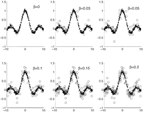
Fig. 2. Data generated by “sinc” function with additive noise of various levels of outliers in Example 1; (dotted-N(0; 0:05 ), (normal), and circle-N(0; 0:2 ) (outliers).

similar to

Huber

’s cost function, because both are based on

l

₁

norm

of errors for larger errors. Note that the

"

-insensitive function is not a

smooth function, and cannot be fitted into M-estimator family, in which

the derivative information of the loss function is basic information in

evaluating the robustness of M-estimator. It is also not suitable for many

optimization procedures, which require derivative information, to be

applied. Instead of using

"

-insensitive cost function, the Huber cost

function has been used in support vector machine (SVM) regression

that is solved by using a recurrent neural network [19].

IV. NUMERICAL

EXAMPLES

Example 1:

Consider using an RBF network to approximate the

“sinc” function

[image:5.594.306.548.345.538.2]

TABLE I

RMS ERRORS ANDMODELSIZE OFDERIVEDMODELSWITHRESPECTIVE TOTRUEFUNCTIONz(EXAMPLE1)

1000 training data

y(x)

were generated from

y(x) = z(x) +

, using

uniformly distributed random

x 2 [010; 10]

. The additive noise

is

a Gaussian mixture that mixes two types of noises, a larger portion of

normal noise with smaller variance and a smaller portion of noise with

higher variance. i.e.

N(0; 0:2

2

) + (1 0 )N(0; 0:05

2

)

, where

0 < < 0:2

as a small number to denote the contamination ratio, such

that

has the probability

(10 )

of being drawn from

N(0; 0:05

2

)

(as

“normal”), and a probability

of

N(0; 0:2

2

)

(as “outliers”).

For various levels of contamination ratio

, 1000 noisy observations

were generated and divided into a training data set of 500 data points

and a test data set of 500 data points. The 500 training data points

is shown in Fig. 2 for different

. For each case, the proposed

algo-rithm is applied based on the RBF network. All the training data points

are used as the candidate center set

c

i

s, with

p

k

(x(t))

constructed

using Gaussian function

p

_k

= (x; c

_k

) = expf0kx 0 c

_k

k

2

=h

2

g

.

The width

h = 1

is fixed for simplicity. Note that by removing the

IRLS inner loop of the algorithm, the procedure simply reduces to OFR

with D-optimality algorithm [13]. For comparison the SVM regression

approach was applied, with the same Gaussian function

k(x; c

_k

) =

expf0kx0c

k

k

2

=h

2

g

, and

h = 1

, as kernels. The parameters in SVM

regression was set as

" = 0:06

and

C = 1

, as these values give the

best tradeoff between model sparseness and generalization by trial and

error.

With various values of

as different level of bad data conditions,

the proposed algorithm is compared with OFR with D-optimality

al-gorithm using only least squares estimates and SVM regression. With

a predetermined small number

= 0:001

, all of the derived models

based on OFR algorithm have the number of centers in the range of

n

= 21 22

, but the model size of SVM regression range from

n

= 123 176

. The root of mean squares (RMS) errors of a range

of data conditions are listed in Table I. It is seen that the proposed

algorithm is most robust to outliers when the data contains

approxi-mately 10% outliers. To achieve better performance for M-estimators,

it is useful to slightly adjust tuning constants because these are set for

95% efficiency when data is normal. As data distribution is unknown

these values can be adjusted via iterations and cross-validation. For the

training data set as shown in Fig. 2 with

= 0:1

, the model predicted

output by using the proposed algorithm with Turkey bisquare

M-esti-mators is shown in Fig. 3. For the best results in term of sparseness

and efficiency, OFR based algorithms are better than SVM regression.

The SVM regression is very robust even with worst data condition, and

gives consistent results for all data conditions.

Fig. 3. Bisquare M-estimator model predictions with = 0:1and true functions (Example 1).

[image:7.594.89.510.64.272.2]

Fig. 4. Automobile MPG data (circle: original data; and dotted: synthetical outliers).

TABLE II

RMS ERRORS ANDMODELSIZE OFDERIVEDMODELSWITHRESPECTIVE TO MPG DATAOUTPUT(EXAMPLE2)

i.e. each input has a width with a similar scale of its standard

de-viation. For both the original data and modified data, four types

of algorithms were applied and the modeling results were listed

in Table II. In the modeling original data without outliers, a

pre-determined small number

= 0:01

was used for all OFR based

algorithms. In the modeling data with outliers, it was found that

the setting of

= 0:01

would terminate at a model with too small

model size with insufficient approximation accuracy, so

= 0:0001

was used to allow larger models and better approximation

accu-racy. In the SVM regression approach, the same Gaussian function

k(x; c

k

) = expf0(x 0 c

k

)

T

diagf50; 500; 5g(x 0 c

k

)g

was used,

and the parameters in SVM regression was set as

" = 3

and

C = 10

.

It is shown that the proposed algorithm and SVM are robust to outliers

than least square parameter estimates, in the sense that they are less

vulnerable to the change in data’s deviation from its original data. The

OFR based algorithms produce more sparse models than that of SVM

regression for all cases.

V. CONCLUSIONS

In this correspondence, a new OFR model identification algorithm

is introduced. The OFR, often based on the modified Gram–Schmidt

procedure, is an efficient method incorporating structure selection and

parameter estimation simultaneously. The proposed algorithm includes

M-estimator by using an IRLS algorithm inner loop based on the

mod-ified Gram–Schmidt procedure. D-optimality as a model structure

ro-bustness criterion is used in model selection. In this manner the

pro-posed approach extends the use of the OFR algorithm for

parsimo-nious model structure determination even in bad data conditions via

the derivation of parameter M–estimators with inherent robustness to

outliers. Numerical examples have shown that the proposed algorithm

has improved performance than OFR with least squares parameters as

data condition deteriorates.

ACKNOWLEDGMENT

The authors wish to thank the referees for their suggestions which

greatly improved the quality of this paper.

REFERENCES

[1] P. J. Huber,Robust Statistics. New York: Wiley, 1981.

[2] J. T. Connor and R. D. Martin, “Recurrent neural networks and robust time series prediction,”IEEE Trans. Neural Netw., vol. 5, no. 2, pp. 240–253, Mar. 1994.

[3] J. H. Chen, C. S. Chen, and Y. S. Chen, “Fast algorithm for robust tem-plate matching with m-estimators,”IEEE Trans. Signal Process., vol. 51, no. 1, pp. 230–243, Jan. 2003.

[4] A. B. Hamza, H. Krim, and G. B. Unal, “Unifying probabilistic and variational estimation,”IEEE Signal Process. Mag., vol. 19, pp. 37–47, Sep. 2002.

[5] A. C. Atkinson and A. N. Donev,Optimum Experimental Designs. Ox-ford, UK: Clarendon Press, 1992.

[6] S. Chen, S. A. Billings, and W. Luo, “Orthogonal least squares methods and their applications to nonlinear system identification,”Int. J. Contr., vol. 50, pp. 1873–1896, 1989.

[7] S. Chen, Y. Wu, and B. L. Luk, “Combined genetic algorithm opti-mization and regularized orthogonal least squares learning for radial basis function networks,”IEEE Trans. Neural Netw., vol. 10, no. 6, pp. 1239–1243, Nov. 1999.

[8] M. J. L. Orr, “Regularization in the selection of radial basis function centers,”Neural Computat., vol. 7, no. 3, pp. 954–975, 1995. [9] X. Hong, M. Brown, S. Chen, and C. J. Harris, “Sparse model

identifica-tion using orthogonal forward regression with basis pursuit and [d]-opti-mality,” IEE Proc. Contr. Theory Applicat., vol. 151, no. 4, pp. 491–498, 2004, submitted for publication.

[10] S. Chen, X. Hong, and C. J. Harris, “Sparse kernel regression modeling using combined locally regularised orthogonal least squares and d-opti-mality experimental design,”IEEE Trans. Autom. Contr., vol. 48, no. 6, pp. 1029–1036, Jun. 2003.

[12] X. Hong and C. J. Harris, “Nonlinear model structure detection using op-timum experimental design and orthogonal least squares,”IEEE Trans. Neural Networks, vol. 12, no. 2, pp. 435–439, Mar. 2001.

[13] , “Nonlinear model structure design and construction using orthog-onal least squares and d-optimality design,”IEEE Trans. Neural Netw., vol. 13, no. 5, pp. 1245–1250, Sep. 2001.

[14] V. Vapnik,The Nature of Statistical Learning Theory. New York: Springer-Verlag, 1995.

[15] K. R. Müller, S. Mika, G. Rätsch, K. Tsuda, and B. Schölkopf, “An introduction to kernel-based learning algorithms,”IEEE Trans. Neural Netw., vol. 12, no. 2, pp. 181–201, Mar. 2001.

[16] K. L. Lee and S. A. Billings, “Time series prediction using support vector machines, the orthogonal and the regularized orthogonal least squares algorithms,”Int. J. Syst. Sci., vol. 33, no. 10, pp. 811–821, 2002.

[17] C. J. Harris, X. Hong, and Q. Gan, Adaptive Modeling, Estima-tion and Fusion From Data: A Neurofuzzy Approach. New York: Springer-Verlag, 2002.

[18] M. Brown and C. J. Harris,Neurofuzzy Adaptive Modeling and Con-trol. Englewood Cliffs, NJ: Prentice-Hall, 1994.

[19] Y. Xia and J. Wang, “A one-layer recurrent neural network for support vector machine learning,”IEEE Trans. Syst., Man, Cybern., B, Cybern., vol. 34, no. 2, pp. 1261–1269, Apr. 2004.