A Comparison of Adaptive Beamforming Implementations for Wideband Scenarios

A COMPARISON OF ADAPTIVE BEAMFORMING

IMPLEMENTATIONS FOR WIDEBAND SCENARIOS

Stephan Weiss

, Choo Leng Koh

and Wei Liu

∗_{Communications Research Group, School of ECS, University of Southampton, UK} †_{Department of Electronic and Electrical Eng., University of Sheffield, Sheffield, UK}

Keywords: Broadband beamforming, adaptive signal process-ing, efficient implementation, subband processprocess-ing, frequency domain processing.

Abstract

In this paper, we compare low cost implementations of wide-band adaptive beamformers utilising the generalised sidelobe canceller (GSC) in combination with the least-mean squares algorithms. DFT based techniques suffer from unjustified nar-rowband assumptions. We therefore derive and investigate an overlap-save implementation of the GSC, which offers a steady state suppression of jammers equivalent to a time domain GSC but may be prone to slow convergence. Finally, subband tech-niques offer a more robust convergence trade-off for a some-what higher computational cost. Analysis and simulation re-sults revealing some of the algorithms’ properties are presented.

1 Introduction

Ultra-wideband (UWB) communications offers a radically dif-ferent approach to wireless communication compared to con-ventional narrowband systems. This fast emerging technol-ogy with uniquely attractive features invite major advances in wireless communications, networking, radar, imaging and po-sitioning systems [1]. However, for this technology to achieve high spectral and spatial resolution, the array usually requires a considerable temporal and spatial dimension. Thus, a larger number of sensors,_M, and tap delay line (TDL) elements,_L, results in a very large computational complexity of wideband beamforming algorithms, inhibiting the deployment of pow-erful techniques such as recursive least squares (RLS) algo-rithms.

To reduce the computational complexity of wideband beam-forming algorithms, transformations can be applied to the TDL elements of each sensor. For example, the discrete Fourier transform (DFT) yields frequency bins, on which independent narrowband beamforming algorithms can be performed [3, 4, 5], yielding tremendous savings [6]. However, the suboptima-lity of these narrowband solutions with respect to the wide-band problem, as established in e.g. [4, 7, 8], requires slid-ing window and block processslid-ing implementations [5] to be replaced by algorithms based on overlap-add or overlap-save techniques [8, 9, 10]. This step enhances the mean square error

This work was supported by the U.K. MoD’s Corporate Research Pro-gramme.

performance, but increases the computational load compared to sliding window and block processing. Further, subband trans-formations for adaptive filtering [11] can be applied to wide-band beamforming [12, 13, 14]. There, filter banks with a high frequency selectivity produce non-critically decimated alias-free subband signals, which can be processed independently. Although the various subbands will require wideband beam-forming algorithms, a considerably reduced temporal dimen-sion can be achieved [7, 13].

This paper performs a comparative study of the various methods — in terms of computational cost, convergence speed, and steady-state error — by example of the generalised side-lobe canceller (GSC) [2, 15]. Sec. 2 briefly reviews the GSC’s structure, while the various low-complexity realisations are dis-cussed in Sec. 3. Simulations in Sec. 4 will provide insight into the performance of various systems, and conclusions be drawn in Sec. 5.

2 Wideband Beamforming via the Generalised

Sidelobe Canceller

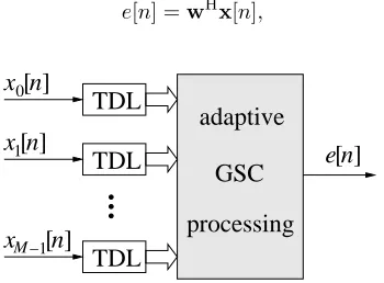
We consider the wideband beamforming structure depicted in Fig. 1, which acquires a spatio-temporal waveform by means of Msensor signals_xm[_n],_m= 0(1)_M−1and fed into tapped-delayed lines (TDLs) of dimension_L. At each discrete time instance_n, an_{M L}dimensional data vector

x[_n] = xT 0[n]x

T

1[n] . . . x T

M−1[n]

T

(1)

xm[n] = [xm[n]xm[n−1] . . . xm[n−L+1]]T (2)

is passed to the beamforming processor. We consider a linear wideband beamformer, where a a linear output

e[n] =wHx[n], (3)

TDL

TDL

TDL

[n]

e

[n]

x

[n]

x

[n]

x

processing

GSC

adaptive

is formed by a scalar product with the beamforming weights in w,

w = wT 0 w

T 1 . . . w

T

M−1

T

(4)

wm = [wm,0wm,1 · · · wm,J−1] T

.

Exemplarily, we want to consider the linearly constrained min-imum variance (LCMV) beamforming problem [19],

min

w w

H_R

xxw subject to CHw=f _, (5) whereR_xx = Ex[n]xH_[

n]is the covariance matrix, C ∈

CMJ×r_{the constraint matrix andf ∈ C}r_{the response vector}

for linearly independent constraints.

The generalised sidelobe canceller (GSC) transforms (5) into an unconstrained optimisation problem by projecting the M Lelement data vector by a blocking matrixB∈CML×ML−r onto a subspace independent of the constraints, i.e. u[_n] = BH_x[

n], and by a quiescent vectorwq to obtain the signal of

interest plus interference,_d[_n] =wH

qx[n]. Unconstrained

op-timisation of the output

e[n] =d[n]−wHau[n] (6)

can then be performed to linearly combine the blocking matrix outputs by coefficients inwa ∈ CML−rto minimise any

in-terference remaining in d[n]in the mean square error (MSE) sense [2, 15]. With the projections amounting to(_{M L})2

mul-tiply-accumulates (MACs), the optimisation can be performed, for example, by a normalised LMS algorithm with a complex-ity of approximately3_{M L}MACs.

3 Efficient Implementations

3.1 Independent Frequency Bin Processing

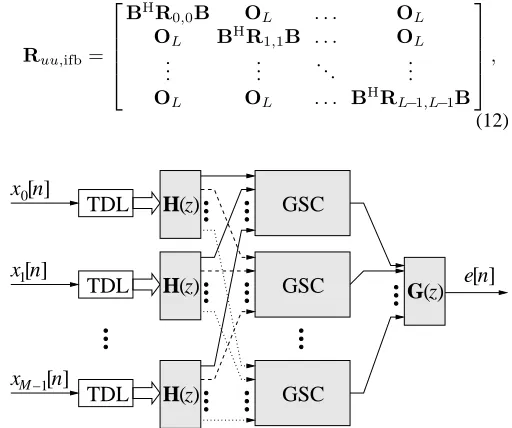
A class of popular beamforming algorithms applies DFTs to each TDL, and independently processes the resulting frequency bins by _Lnarrowband beamforming algorithms, e.g. a GSC, as shown in Fig. 2, withH(_z)representing an _L-point DFT matrix [3, 4, 5]. The resulting cost for processing the signal in blocks of_Lsamples accrues to

Cfb,block= (M + 1) log2L+M 2_{+ 3}

M (7)

complex MACs per fullband sampling period. A sliding win-dow version of this algorithm computes the DFTs at each time instance_n, and replaces the IDFT at the beamformer output in Fig. 2 by a simple summation [5], yielding a slightly higher cost of

Cfb,sliding=M Llog2L+LM 2_{+ 3}

LM (8)

MACs per fullband sampling period.

In both block and sliding window DFT implementations, we use a vectorxfdto denote the input data to the GSC

beam-former.

xfd[n] =P

⎡ ⎢ ⎣

TL 0

. ._.

0 TL

⎤ ⎥

⎦·x[n], (9)

whereT_Lis anL-point DFT matrix applied to each TDL and Pa permutation matrix such that xfd[n]is ordered w.r.t.

fre-quency bins. The latter vector contains the_M sensor compo-nents for the first frequency bin in its first_M elements, and so forth until the last_M elements are occupied by the_M sensor components of the_Lth frequency bin.

By applying a DFT to the constraint equation in (5), con-straints for sliding window and block processors can be de-rived. If the signal of interest illuminates the array from broad-side, the _r = _L constraints are decoupled and identical for every frequency bin. As a result, the input to the adaptive GSC processor can be denoted as

ufd[n] =

⎡ ⎢ ⎣

BH ₀

. ._.

0 BH

⎤ ⎥ ⎦

BH fd

xfd[n] , (10)

withufd[n] ∈ C(M−1)L andB ∈ CM×M−1. Note that the

blocking matrixBapplied to each frequency bin is different from the blocking matrix defined in Sec. 2. Therefore, the co-variance matrixR_uu,fd=E

ufd[n]·uHfd[n]

is given by

Ruu,fd =BHfd

⎡ ⎢ ⎢ ⎢ ⎣

R0,0 R1,0 . . . RL−1,0

R0_,1 R1_,1 . . . R_L−1_,1

..

. ... . .. ... R0,L−1 R1,L−1 . . . RL−1,L−1

⎤ ⎥ ⎥ ⎥ ⎦Bfd

(11) whereR_i,jare_M×_M correlation matrices between frequency bins i and j of the different sensor signals prior to passing the blocking matrixBfd.

Block and sliding window processing neglect any corre-lation between frequency bins. With this approximation, the covariance matrix to the resulting independent frequency bin (IFB) processorR_uu,fdis forced to attain the form

Ruu,ifb=

⎡ ⎢ ⎢ ⎢ ⎣

BH_R

0_,0B O_L . . . O_L

OL BHR1,1B . . . OL

..

. ... . .. ... OL OL . . . BHRL−1,L−1B

⎤ ⎥ ⎥ ⎥ ⎦,

(12)

TDL

TDL

TDL

[n]

x

[n]

1

x

_e

_[n]

[n]

x

(z)

H

(z)

H

(z)

H

(z)

G

GSC

GSC

GSC

i.e. any correlation between binsiandj=iis neglected. How-ever, due to the high sidelobes in the DFT’s frequency response characteristics as depicted in Fig. 3, adaptive algorithms suf-fer from spectral leakage — limiting their convergence [16] — and potentially need a substantial amount of degrees of free-dom to approximately suppress even low rank interferers [7]. Recently, such failures have generally been attributed to the application of essentially narrowband processing to wideband problems [8].

3.2 Overlap-Save DFT Implementation

In order to overcome the problem of inter-frequency bin cor-relations being neglected, overlap-add or overlap-save meth-ods can be applied to accurately address wideband problems in the DFT-domain [8, 9, 10]. Overlap-add and overlap-save techniques exploit the Toeplitz nature of the of data matrix, transforming it to a circulant form by increasing the DFT to

2Lpoints. Unlike the circular convolution between the signals xm[n] and the filters following each sensor implemented by the previously outlined methods, they now realise a linear con-volution [9]. By rigorously minimising time domain criteria, such as the mean square error, expressed in the DFT domain, exact wideband DFT domain methods can be attained and, if required, subsequently simplified [8].

3.2.1 Exact Frequency Domain Formulation

We first introduce a block processing notation by stacking the outputs_e∗[_nL]_{, e}∗[_nL+ 1]_, · · ·_{, e}∗[_nL+_L−1]into a vector e[_n]∈CL_{, yielding}

e[_n] =M−

1

m=0

XH

m[n]wm, (13)

where with (2)

Xm[n] = [xm[nL] xm[nL+1] · · · xm[nL+L−1]] . (14)

0 0.1 0.2 0.3 0.4 0.5 0.6 0.7 0.8 0.9 1 −25

−20 −15 −10 −5 0 5

normalised angular frequency Ω / π

|Fi

(e

j

Ω| / [dB]

Fig. 3. Filter bank characteristic of a 16-point DFT.

We can expand the convolutional matricesX_m[n]to a circulant form [20] and write the output of the beamformer as

v e[n]

=

M−1

m=0

_˜

XH

m[n] XHm[n]

XH

m[n] X˜Hm[n]

·

wm

0

(15)

wherevis an arbitrary_J element vector andX˜_mis a Toplitz matrix using the data samples ofX_m except for an arbitrary element along the main diagonal. Note that with a2_Lpoint DFT matrix T, the circulant property can be exploited such that

Γ_m[_n] = T·

_˜

XH

m[n] XHm[n]

XH

m[n] X˜Hm[n]

·TH ₍₁₆₎

= diag

TJ

xm[nL+L]

xm[nL]

(17)

takes on a diagonal form [20], wherebyJis a reverse identity. Therefore, the definition of a DFT domain error vectore[n]∈

C2L_{leads to}

e[_n] = T

0

en

= T

0L×L 0L×J

0L×L IL

TH

G

·T

v en

= G M−

1

m=0

Γ_m[_n]·T

wm

0

=G Γ[_n]w (18)

in dependency of the frequency domain coefficientsw∈C2ML

withG∈C2L×2L_{, andΓ[}

n]∈C2L×2ML_.

To formulated the constraint equation with the frequency domain variables,

CH_w=

M−1

m=0

CH

m·wm=f (19)

whereby the original matrix equation can be separated into_M additive components. Note thatC_m ∈ CL×rhas an arbitrary form (in particular not Toeplitz), where_ris the number of lin-early independent constraints. In terms of the DFT domain co-efficients, we have

M−1

m=0

CH

m 0r×J w₀m

=f (20)

or

M−1

m=0

CH

m 0r×J THwm=CHw=f , (21)

whereC∈C2ML×ris the new constraint matrix

C=

C0

0L×r H

TH _{· · ·}

CM−1

0L×r H

TH

H

(22)

3.2.2 Overlap-Save GSC

The LCMV formulation equivalent to the time domain but us-ing frequency domain variables is now given by

min

w E

eH_[

n]e[n]= min_w wHRw, (23)

subject toCHw = f, where R = EΓ[_n]HGHGΓ[_n] = EΓ[_n]H_GΓ[

n].

Analogously to the time domain formulation of the GSC, the weight vector_wis separated into two orthogonal compo-nents,w=wq−v, with a quiescent vectorwqrepresenting a

projection onto the constraints, and a projection away from the constraints,−v, given by

v=Bwa (24)

utilising the blocking matrixB=span{C⊥}, which spans the nullspace of the constraint matrixC.

Therefore, with (18), the beamformer output is given by

e[n] =G Γ[n] wq−Bwa

. (25)

Analogously to a time domain LMS algorithm, by using the instantaneous squared error as a cost function_ξ =eH_[

n]e[n] we obtain a stochastic gradient

ˆ

∇ξ = _∂w∂ξ_∗

a

= −BH _ΓH_[

n]e[n] (26)

whereGH_{G=Ghas been exploited. The update equation for}

wacan then be written as

wa[n+ 1] =wa[n] +μB H_ΓH_[

n]e[n] (27)

The computational cost of this exact frequency domain GSC algorithm has been addressed in [22] and accrues to

Cfd,os= 2M(4M L−2r+ log2L+ 3) + 4 log2L+ 6 (28)

complex MACs per fullband sampling period.

3.2.3 Covariance Matrix

To determine the input covariance matrix to the adaptive pro-cess, we follow a proof of convergence in the mean similar to the LMS algorithm [21]. If the MMSE solution is subtracted both sides of (27), it can be shown that

˜

wa[n+ 1] = ˜wa[n]−μB

H_EΓH_[

n]GΓ[n]

B_w˜_a[_n] = I−μBH_EΓH_[

n]GΓ[n]

B_w˜_a[_n](29)

with_w˜_a[_n] =E

wa[n]−wa,opt

, wherew_a,optis the MMSE solution. If the solution in (29) is compared to the structurally identical derivation for the LMS, the term

Ros=BHE

ΓH_[

n]GΓ[n]

B ∈C2ML−r×2ML−r ₍₃₀₎

0 0.1 0.2 0.3 0.4 0.5 0.6 0.7 0.8 0.9 1 −100

−90 −80 −70 −60 −50 −40 −30 −20 −10 0 10

normalised angular frequency Ω / π

|H

k

(e

j

Ω| / [dB]

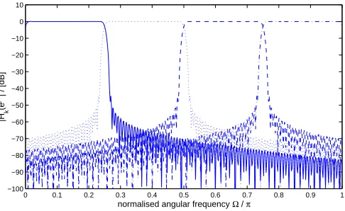
Fig. 4. Filter bank characteristic(_K= 8_{, N} = 6)_.

can be identified as the covariance matrix in the overlap-save frequency domain implementation of the GSC. Note that no approximation have been made in the derivation of the overlap-save method with respect to the original time domain MSE, and that Rosis not forced to be of block diagonal form as in the

standard frequency domain approach of Sec. 3.1.

3.3 Independent Subband Processing

In subband adaptive beamforming, the blocksH(z)in Fig. 2 represent_K-channel analysis filter banks which are non-critically decimated by a factor_{N < K}. These filter banks can be de-rived from a real value prototype FIR filter by a generalised discrete Fourier transform (GDFT), according to [17]. The re-dundancy of the filter banks can be exploited to attain a high frequency selectivity where sidelobes between adjacent bins are kept to a minimum as illustrated in Fig. 4.

Due to the high sidelobe attenuation, the resulting subbands only overlap with adjacent bands and possess a sufficiently high stopband attenuation elsewhere. The covariance matrix of the filter bank outputs, given byR_xx,sub=E

xsub·xHsub

∈

CKML/N×KML/N_{, therefore takes the structure of}

Rxx,sub=

⎡ ⎢ ⎢ ⎢ ⎢ ⎢ ⎢ ⎢ ⎢ ⎣

R0_,0 R1_,0 0_J . . . 0_J R_K−1_,0

R0_,1 R1_,1 R2_,1 0_J 0_J

0J R1,2 R2,2 . .. ...

..

. . .. . .. . .. _0J 0J . .. RK−2_,K−2 R_K−1_,K−2

R0,K−1 0J . . . 0J RK−2,K−1 RK−1,K−1

⎤ ⎥ ⎥ ⎥ ⎥ ⎥ ⎥ ⎥ ⎥ ⎦

(31) with_J =_{M L/N}, where

xT

sub[v] =

x0[v]x1[v] · · · xK−1[v]

with (32) xT

k[v] =

x0,k[v]x1,k[v] · · · xM−1,k[v]

, xT

m,k[v] =

ˆ

xm,k[v] ˆxm,k[v−1] · · · xˆm,k[v−L/N+1].

The vectorxT_m,k[_v] contains data inside a TDL formed from the_mth_{sensor signal in the}

kth_{subband, with}

processing, the subband signals are still considered wideband — although with a reduced bandwidth as evident from Fig. 4 — thus motivating the need for wideband processing in the sub-band domain. However, due to the reduced sub-bandwidth note that the length of TDL for each subband channel is now ap-proximately_Ntimes shorter than the fullband case [13].

The essence for computational efficiency in subband-based beamforming is the independent processing of subband signals. Although adjacent subband signals are correlated, the off-block diagonal terms in (31) are due to redundancy in the overlap regions, and will disappear if the main block diagonal terms Rk,k, k = 0(1)K−1 are suppressed, i.e.R_xx,subis

rank-deficient. Therefore, different from critically decimated DFT domain processing, the off-block-diagonal terms in (31) can be neglected from processing without incurring a penalty, and a separate beamforming algorithm can be operated in each sub-band [14, 13].

The covariance matrix seen by the adaptive filter input is given by

Ruu,sub=BHsb Rxx,subBsb (33)

with a block diagonal blocking matrix

Bsb=

⎡ ⎢ ⎣

B0 0

. ._. 0 BK−1

⎤ ⎥

⎦ (34)

consisting of the blocking matricesB_k ∈ CML/N×(M−1)L/N

, k= 0(1)K−1. Hence,R_uu,subretains the structure ofR_uu,sub

and its redundancy. With the temporal dimension of the sub-band beamformers reduced by a factor of approximately_Nand an_Ntimes slower update rate due to decimation, the computa-tional complexity of this approach accrues to

Csb =

1

N[(M + 1)(4Klog 2(K) + 4K+Lp) +

+ K(M L/N)2+KM L/N] (35)

MACs, whereby _Lp is the length of the filter bank’s proto-type and the filter bank implementation is based on a gener-alised DFT modulation permitting a computationally inexpen-sive polyphase realisation. The cost in (35) also includes the reconstruction of the beamformer output via a synthesis bank G(_z), as indicated in Fig. 1.

4 Performance Comparison

4.1 Computational Complexity

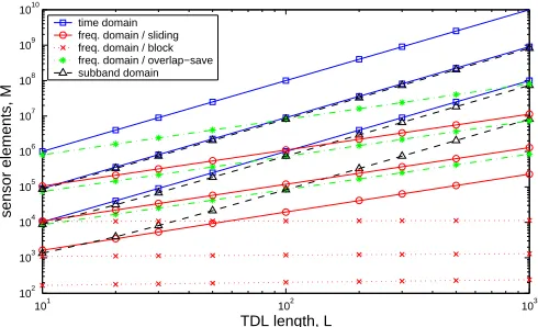
A comparison of complexity between the various GSC imple-mentations is provided in Fig. 5 in dependence on the tem-poral dimension_L and the number of sensor elements_M of the beamformer. The time domain implementation is the most costly realisation, while the lowest cost is afforded by the in-dependent frequency bin processor in block mode. The sliding window independent frequency bin processor is more costly than the latter, but still provides a benefit in terms of complex-ity of overlap-save and the subband realisation, which is based

101 ₁₀2 ₁₀3

102 103 104 105 106 107 108 109 1010

TDL length, L

sensor elements, M

time domain freq. domain / sliding freq. domain / block freq. domain / overlap−save subband domain

Fig. 5. Computational complexities in MACs of the various GSC implementations in dependence on the TDL length_Land M = 10,_M = 30, and_M = 100sensor elements each. The lowest curve reverse to_M = 10, the highest of each kind to M = 100.

on a filter bank withK = 16channels decimated byN = 14 based on a prototype with_Lp= 448coefficients.

4.2 Final MSE

Taking the performance of the time domain beamformer as a benchmark, we assess the possible final MSE of the various implementations. Since the overlap save technique optimises the time domain cost function, its steady state performance can be expected to be similar to the time domain solution. A differ-ence arises from the doubling of the adaptive parameters from M L−relements inw_a[n]to2M L−Lelements inw_a[n], resulting in a potentially larger excess mean square error [21].

Block and sliding window independent frequency bin im-plementations suffer from the forced block-diagonalisation of the covariance matrixR_uu,ifbin (12), which is justified only

if the input signal consists of frequencies coinciding with fre-quency bins. If the input signal violates this condition, then the MSE performance will be reduced with respect to the time do-main approach. A shown in [7], potentially a rank one source could require all degrees of freedom available in the beam-former [7], and hence with the exhaustion of available degrees of freedom in the system, the steady state MSE performance can be poor.

The subband approach is based on the tri-block diagonal covariance matrix in (33). As evident from the filter bank char-acteristic in Fig. 4, the stopband level of the bandpass filters determines how well the idealised zero matrices0_ML/Nare ap-proximated, as they will determine the MSE bound [16]. Thus the MSE performance of the subband GSC can be controlled by the filter bank design, in contrast to sliding window and block processing methods.

4.3 Convergence Speed

0 1000 2000 3000 4000 5000 6000 −5

0 5 10 15 20 25 30 35 40 45 50

discrete time n

ensemble MSE / [dB]

time domain freq. domain/sliding freq. domain/block freq. domain/overlap save subband domain

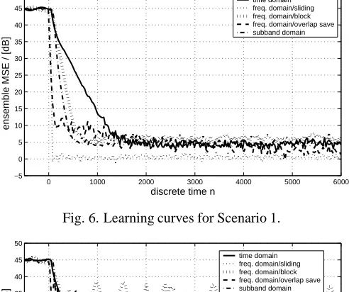
Fig. 6. Learning curves for Scenario 1.

0 1000 2000 3000 4000 5000 6000 −5

0 5 10 15 20 25 30 35 40 45 50

discrete time n

ensemble MSE / [dB]

time domain freq. domain/sliding freq. domain/block freq. domain/overlap save subband domain

Fig. 7. Learning curves for Scenario 2.

consider an array with_M = 10linear uniformly spaced sensors followed by TDLs of length_L= 32. In the case of a subband implementation, we utilise a filter bank with prototype length Lp = 96decomposing signals into_K = 8 subbands deci-mated by_N = 6. The computational complexity of the various schemes is summarised in Tab. 1. The signal of interest is at the array’s broadside, while 10 narrowband jammers impinge from -20◦at an SINR of -45 dB. Additionally, the array is corrupted by uncorrelated noise at an SNR of -6 dB. Below, we consider two scenarios for the interferers.

Scenario 1. All interferers sit on frequency bins, i.e. at integer multiples of Ω = 2_π/L, and not in the overlap re-gion of the analysis filter banks of the subband implementa-tion. The mean squared residual error (MSE), i.e. the beam-former output minus the signal of interest, over an ensemble of 100 simulations is shown in Fig. 6. For the frequency domain

Table 1. Computational cost of various beamformers.

structure MAC/sample rel. cost time domain 103360 100.00% freq. domain/block 185 0.18% freq. domain/sliding 5760 5.57% freq. domain/overlap save 416 0.40% subband domain 4416 4.27%

methods, the interferers sit on frequency bins and can be nulled out fast and with a single degree of freedom (DOF) – the data covariance matrix at the blocking matrix output is diagonal, and no approximation error is made by neglecting correlations between different frequency bins. The subband method con-verges somewhat fast than the time domain approach due to the prewhitening effect of the decomposition.

Scenario 2. All interferers lie outside the frequency bins and coincide with the overlap region of the filter banks. As can be seen in Fig. 7, the time domain algorithm is unaffected. In the subband scheme each interferer will appear in the two sub-bands sharing the overlap region, and two DOFs are required to suppress each rank-one interferer [7]. Since the order of the subband beamformer is large enough to provide the DOFs, the convergence characteristic is not substantially different from Fig. 6. For the DFT based approaches, block processing and sliding window methods fail due to neglecting the correlations between frequency bins. All temporal DOFs are needed to sup-press a single interferer, otherwise only a limited level of at-tenuation can be achieved. The overlap-save method reaches a satisfactory steady-state MSE, but due to a large dynamic range in the excitation of the various frequency bins due to spectral leakage as well as block adaptation [10], convergence is slow.

5 Conclusions

A number of different beamformer implementations have been reviewed and compared. DFT-based techniques, in particu-lar block processing, offer high computational savings. How-ever, if the jammer signal components do not coincide with frequency bins, block and sliding window methods suffer from unjustified narrowband approximations. The presented overlap-save method guarantees a better steady-state value, but can incur slow convergence, while the subband approach offers a very robust performance at a somewhat higher cost, although still inexpensive and consistently faster in terms of its conver-gence compared to a time domain implementation.

6 Acknowledgement

We would like to thank Prof. Ian K. Proudler and Prof. John G. McWhirter of the Advanced Signal Processing Group, Qine-tiQ Ltd., Malvern, UK, for their support and technical input.

References

[1] Liuqing Yang and G. B. Giannakis, “Ultra-wideband communications: an idea whose time has come,” IEEE

SP Mag, 21(6): 26–54, 2004.

[2] B. D. Van Veen and K. M. Buckley, “Beamforming: A Versatile Approach to Spatial Filtering,” IEEE ASSP

Mag, 5(2): 4–24, 1988.

[4] David Nunn, “Suboptimal Frequency-Domain Adaptive Antenna Processing Algorithm for Broad-Band Environ-ments,” IEE Proc. F: Radar Sig. Proc., 134(4): 341–351, 1987.

[5] H. L. Van Trees, Optimum Array Processing, Wiley, 2002.

[6] L. C. Godara and M. R. S. Jahromi, “Limitations and Capabilities of Frequency Domain Broadband Constraint Beamforming Schemes,” IEEE Trans. SP, 47(9): 2386– 2395, 1999.

[7] S. Weiss and I. K. Proudler, “Comparing Efficient Broad-band Beamforming Architectures and Their Performance Trade-Offs,” in Proc. 14th Int. Conf. DSP, Santorini, Greece, 2002, 1: 417–423.

[8] W. Kellermann and H. Buchner, “Wideband Algorithms Versus Narrowband Algorithms for Adaptive Filtering in the DFT Domain,” in Asilomar Conf. Sig. Sys. Comp., 2003.

[9] R. E. Crochiere and L. R. Rabiner, Multirate Digital

Sig-nal Processing, Prentice Hall, 1983.

[10] J. J. Shynk, “Frequency-Domain and Multirate Adaptive Filtering,” IEEE SP Mag., 9(1): 14–37, 1992.

[11] W. Kellermann, “Analysis and Design of Multirate Sys-tems for Cancellation of Acoustical Echoes,” in Proc.

IEEE ICASSP, NY, 1988, 5: 2570–2573,

[12] F. Lorenzelli, A. Wang, D. Korompis, R. Hudson, and K. Yao, “Subband Processing for Broadband Microphone Arrays,” J. VLSI Sig. Proc. Sys. for Signal, Image, and

Video Tech., 14(1): 43–55, 1996.

[13] S. Weiss, R. W. Stewart, M. Schabert, I. K. Proudler, and M. W. Hoffman, “An Efficient Scheme for Broad-band Adaptive Beamforming,” in Proc. Asilomar

Conf. Sig. Sys. Comp., Pacific Grove, CA, 1999, 1: 496–

500.

[14] B. Farhang-Boroujeny and Z. Wang, “Adaptive Filtering in Subbands: Design Issues and Experimental Results for Acoustic Echo Cancellation,” Sig. Proc., 61(3): 213–223, 1997.

[15] L. J. Griffith and C. W. Jim, “An Alternative Approach to Linearly Constrained Adaptive Beamforming,” IEEE

Trans. AP, 30(1): 27–34, 1982.

[16] S. Weiss, A. Stenger, R. W. Stewart, and R. Raben-stein, “Steady-State Performance Limitations of Subband Adaptive Filters,” IEEE Trans. SP, 49(9): 1982–1991, 2001.

[17] M. Harteneck, S. Weiss, and R. W. Stewart, “Design of Near Perfect Reconstruction Oversampled Filter Banks for Subband Adaptive Filters,” IEEE Trans. Circ. & Sys. II, 46(8): 1081–1086, 1999.

[18] C.-L. Koh, Broadband Adaptive Beamforming with Low

Complexity and Frequency Invariant Response, technical

report, Univ. of Southampton, 2004.

[19] O. L. Frost, III, “An Algorithm for Linearly Constrained Adaptive Array Processing,” Proc. IEEE, 60(8): 926– 935, 1972.

[20] G. H. Golub and C. F. Van Loan, Matrix Computations, John Hopkins, 3rd ed., 1996.

[21] S. Haykin, Adaptive Filter Theory, Prentice Hall, 2nd ed., 1991.