Parameterizations for ensemble Kalman inversion

Neil K. Chada∗, Marco A. Iglesias∗∗, Lassi Roininen† and Andrew M. Stuart‡

∗_{Mathematics Institute, University of Warwick, Coventry, CV4 7AL, UK.} ∗∗ _{School of Mathematical Sciences, University of Nottingham,}

Nottingham Park, NG7 2QL, UK.

† _{Department of Mathematics, Imperial College London, London, SW7 2RD, UK.} ‡ _{Computing and Mathematics Sciences, California Institute of Technology,}

Pasadena, CA 91125, USA.

E-mail:

n.chada@warwick.ac.uk

marco.iglesias@nottingham.ac.uk l.roininen@imperial.ac.uk astuart@caltech.edu

Abstract. The use of ensemble methods to solve inverse problems is attractive because it is a derivative-free methodology which is also well-adapted to parallelization. In its basic iterative form the method produces an ensemble of solutions which lie in the linear span of the initial ensemble. Choice of the parameterization of the unknown field is thus a key component of the success of the method. We demonstrate how both geometric ideas and hierarchical ideas can be used to design effective parameterizations for a number of applied inverse problems arising in electrical impedance tomography, groundwater flow and source inversion. In particular we show how geometric ideas, including the level set method, can be used to reconstruct piecewise continuous fields, and we show how hierarchical methods can be used to learn key parameters in continuous fields, such as length-scales, resulting in improved reconstructions. Geometric and hierarchical ideas are combined in the level set method to find piecewise constant reconstructions with interfaces of unknown topology.

PACS numbers: 62M20, 49N45, G5L09.

Keywords: Ensemble Kalman inversion, hierarchical inversion, centered and non-centered parameterizations, discontinuous reconstructions, level set methods.

1. Introduction

1.1. Content

Consider finding u fromy where

y=G(u) +η, (1)

G is a forward map taking the unknown parameter u into the data space, and η

represents noise. Ensemble Kalman inversion is an attractive technique that has shown considerable success in the solution of such problems. Whilst it is derived from the application of Kalman-like thinking, with means and covariances computed from an empirical ensemble, it essentially acts as a black-box derivative-free optimizer which requires only evaluation of the forward map G(·); in practice it can often return good solutions to inverse problems with relatively few forward map evaluations. However the choice of parameterization of the unknown is key to the success of the method. In this paper we will demonstrate how carefully thought out parameterizations can have substantial impact in the quality of the reconstruction.

Although our viewpoint in this paper is to consider Ensemble Kalman inversion as an optimization method, and evaluate it from this perspective, there is considerable insight to be gained from the perspective of Bayesian inversion; this is despite the fact that the the algorithm does not, in general, recover or sample the true Bayesian posterior distribution of the inverse problem. Algorithms that can, with controllable error, approximately sample from the true posterior distribution are commonly referred to as fully Bayesian, with examples including Markov Chain Monte Carlo and sequential Monte Carlo. Ensemble Kalman inversion is not fully Bayesian but the link to Bayesian inversion remains important as we now explain. There is considerable literature available about methods to improve fully Bayesian approaches to the inverse problem through for example, geometric and hierarchical parameterizations of the unknown. The purpose of this paper is to demonstrate how these ideas from Bayesian inversion may be used with some success to improve the capability of ensemble Kalman methods considered as optimizers. In view of the relatively low computational cost of the ensemble methods, in comparison with fully Bayesian inversion, this cross-fertilization of ideas has the potential to be quite fruitful.

1.2. Literature Review

success story for the EnKF has been in weather prediction models [2, 23], but it has also been deployed in numerous applications domains, including the reservoir engineering community [1] and in oceanography [21]. Variants on the idea include the randomized maximum likelihood (RML) method [40], and algorithms such as the ensemble square-root Kalman filter [53].

In this paper we are primarily interested in use of ensemble Kalman methods to study inverse problems for parameter estimation, an approach pioneered for oil industry applications where the inverse problem is known as history matching [32, 40]; the paper [18] contains an insightful analysis of the methodology in the large ensemble limit. In this application domain such inversion methods are sometimes referred to as ensemble Kalman smoothers, although the nomenclature is not uniform. We will simply refer to

ensemble Kalman inversion (EKI). The methodology is formulated quite generally in [26], independently of oil industry applications; and in [25] it is shown that the method performs well as an optimizer but does not capture true posterior uncertainty, in the context of oil industry applications.

The ideas introduced in this paper concerning parameterization are independent of the particular implementation of the EKI method used; in all our numerical experiments we will use the form of iterative regularization proposed by Iglesias [24]. The general philosophy behind the method is that, as the algorithm is iterated, the solution to the inverse problem should approach the truth in the small noise limit, and hence that any regularization introduced should diminish in influence in this limit. However, because the convergence theory for ensemble Kalman inversion is in its infancy, the choice of iterative regularization is made by analogy with classical iterative methods that have been used for inverse problems [5, 6, 22], with the ensemble method using empirical covariances in place of derivatives or adjoints of the forward solver. The resulting iterative method is an ensemble version of the Levenberg-Marquardt algorithm with the inclusion of regularization as in [22].

has been limited to date, with the primary contribution being the work [17] where the methodology was based on building large ensembles from multiple Gaussians assigned different weights. However this work requires that the correct hierarchical parameter is in the ensemble if it is to be successful. We also note that there is some work in hierarchical EnKF within the context of state estimation; see [51] and the references therein.

In addition to hierarchical approaches we will also study geometric parameteriza-tions. These can be of use when the geometric object has known form, such as faults, channels and inclusions, or when it is of unknown topology the level set method may be used [47]. We will build on recent Bayesian implementation of these ideas; see [27, 28] and references therein.

1.3. Contribution of This Work

Our main contribution is to establish the importance of novel parameterizations which have the potential to substantially improve the performance of EKI. Although our perspective on EKI is one of optimization, the methods we introduce are all based on taking established and emerging methods from Bayesian statistics and developing them in the context of the ensemble methods. The connection to Bayesian statistics is exploited to provide insights about how to make these methods efficient. The resulting methods are illustrated by means of examples arising in both electrical impedance tomography, groundwater flow and source inversion. The contributions are:

• We develop hierarchical approaches for EKI, based on solving for the unknown function and unknown scalars which parameterize the prior.

• We generalize these hierarchical approaches to EKI to include unknown fields which parameterize the prior, rather than scalars.

• We demonstrate the key role of choosing non-centered variables when implementing hierarchical methods.

• We show the potential for geometric hierarchical priors, including the level set parameterization, for piecewise continuous reconstructions.

1.4. Organization

1.5. Notation

Throughout the paper we make use of common notation for Hilbert space norms and inner products,k · k,h·i. We will assume thatX and Y are two separable Hilbert spaces which are linked through the forward operatorG :X → Y. This nonlinear operator can be thought of as mapping from the space of unknown parameters X to the observation space Y. Our additive noise for the inverse problems will be denoted by η ∼ N(0,Γ) where Γ : Y → Y is a self-adjoint positive operator. For any such operator we define

h·,·iΓ=hΓ−1/2·,Γ−1/2·i andk · kΓ =kΓ−1/2· k, and for finite dimensions | · |Γ =|Γ−1/2· | with| · |the Euclidean norm. If the Gaussian measure associated toη is supported onY

then we will require Γ to be trace-class; however we will also consider white noise whose support is on a larger space than Y and for which the trace-class condition fails in the infinite dimensional setting.

2. Inverse Problem

2.1. Main Idea

2.1.1. Non-Hierarchical Inverse Problem We are interested in the recovery of u ∈ X

from measurements ofy∈ Ygiven by equation (1) in which, recall,ηis additive Gaussian noise. In the Bayesian approach to inverse problems we treat each quantity within (1) as a random variable. Via an application of Bayes’ Theorem ‡ [13] we can characterize the conditional distribution of u|y via

P(u|y)∝P(y|u)×P(u), (2)

where _P(u) is the prior distribution, _P(u|y) is the posterior distribution and _P(y|u) is the likelihood. Although we view EKI as an optimizer in this paper, the Bayesian formulation of (1) is important because we derive the initial ensemble from the prior distribution _P(u). From an optimization viewpoint, our goal is to make the following least squares objective function small:

Φ(u;y) = 1

2|y− G(u)| 2

Γ. (3)

This (upto an irrelevant additive constant) is the negative log likelihood since it is assumed thatη is a mean-zero Gaussian with covariance Γ.

2.1.2. Centered Hierarchical Inverse Problem In many applications it can be advantageous to add additional unknowns θ to the inversion process. In particular these may enter through the prior, as in hierarchical methods, [42], and we will refer to such parameters as hyperparameters. The inverse problem is then the recovery of

(u, θ) from measurements of y given again by (1). The additional parameterization of the prior results in Bayes’ Theorem in the form

P(u, θ|y)∝P(y|u)×P(u, θ). (4)

Prior samples, used to initialize the ensemble smoother, will then be of the pair (u, θ).

What we will term centered hierarchical methods (a terminology we discuss in Section 3) typically involve factorization of the prior in the form_P(u, θ) = _P(u|θ)_P(θ). From an optimization point of view our goal is again to make the objective function (3) small, but now using hierarchical parameterization to construct the initial ensemble. §

2.1.3. Non-Centered Hierarchical Inverse Problem Another variant of the inverse problem that is particularly relevant for hierarchical methods, in whichθenters only the prior, isnon-centeredreparameterization (a further terminology discussed in Section 3). We introduce the transformation T : (ξ, θ)→u and note that (1) then becomes

y=G(T(ξ, θ)) +η, (5)

and Bayes’ Theorem then reads

P(ξ, θ|y)∝P(y|ξ, θ)×P(ξ, θ). (6)

Prior samples, again used to initialize the ensemble smoother, will then be of the pair (ξ, θ). Typically the change of variables from u to ξ is introduced so that ξ and θ are independent under the prior: _P(ξ, θ) =_P(ξ)_P(θ).As a result the inverse problem (5) is different to that appearing in (1), in terms of both the prior and the likelihood. This non-centered approach is equivalent to the ancillary augmentation technique discussed in [41] which discusses the decoupling ofuand θthrough the variable ξ. From an optimization viewpoint, our goal is to make the following least squares objective function small:

Φ(ξ, θ;y) = 1

2|y− G(T(ξ, θ))| 2

Γ. (7)

In this paper we consider the application of EKI for solution of the inverse problems (1), non-hierarchically and centered-hierarchically, and (5) non-centered hierarchically. Although this method has a statistical derivation, the work in [26, 35] demonstrates that the method may be thought of as a derivative-free optimizer that approximates the least squares problem (3) and (7) rather than sampling from the relevant Bayesian posterior distribution. We will show that the use of iterative EKI, as proposed by Iglesias in [24], can effectively solve a wide range of challenging inversion problems, if judiciously parameterized.

2.2. Details of Parameterizations

In this section we describe in detail several classes of parameterizations that we use in this paper. The first and second are geometric parameterizations, ideal for piecewise continuous reconstructions with unknown interfaces. The third and fourth are hierarchical methods which introduce an unknown length-scale, and regularity parameter, into the inversion. For the two geometric problems we initially formulate in terms of trying to find a functionw:D7→_R,Da subset of_Rd_{, and then reparameterize} w. For the hierarchical problems we initially formulate in terms of trying to find a function u : D 7→ _R, and then append parameters θ and also rewrite in terms of (ξ, θ)7→u.

2.2.1. Geometric Approach – Finite Dimensional Parameterization In many problems of interest the unknown function w has discontinuities, determination of which forms part of the solution of the inverse problem. To tackle such problems it may be useful to write w in the form

w(x) =

n

X

i=1

ui(x)χDi(x). (8)

Here the union of the disjoint sets Di is the whole domain D. If we assume that the

configuration of the Di is determined by a finite set of scalars θ and let u denote the

union of the functionsui and the parametersθ then we may rewrite the inverse problem

in the form (1). The case where the number of subdomains n is unknown would be an interesting and useful extension of this work; but we do not consider it here.

2.2.2. Geometric Approach – Infinite Dimensional Parameterization If the interface boundary is not readily described by a finite number of parameters we may use the level set idea. For example if the fieldwtakes two known valuesw± with unknown interfaces between them we may write

w(x) = w+_Iu>0(x) +w−Iu<0(x), (9)

and formulate the inverse problem in the form (1) foru. This idea may be generalized to functions which take an arbitrary number of constant values, through the introduction of level sets other than u= 0, or through vector level sets functions u.

2.2.3. Scalar-valued Hierarchical Parameterizations To illustrate ideas we will concentrate on Gaussian priors of Whittle-Mat´ern type. These are characterized by a covariance function of the form

c(x, y) =σ2 2

1−α+d/2 Γ(α−d/2)

_|

x−y| `

α−d/2

Kα−d/2

_|

x−y| `

, x, y ∈_Rd, (10)

where K· is a modified Bessel function of the second kind, σ2 > 0 is the variance and

draws from the Gaussian are well-defined and continuous. On the unbounded domain

Rd, samples from this process may be generated by solving the stochastic PDE

(I −`24)2αu=`d/2pβξ, (11)

where ξ∈H−s_{(D),s >} d

2, is a Gaussian white noise, i.e. ξ ∼N(0, I), and

β =σ22

d_πd/2_Γ(α)

Γ(α− d

2)

.

In this paper we will work with the scalar hierarchical parameters α and τ =`−1<sub>.</sub> Putting `=τ−1 _{into (11) gives the stochastic PDE}

C−12

α,τu=ξ, (12)

where the covariance operatorCα,τ has the formCα,τ =τ2α−dβ(τ2I−∆)−α.Throughout

this paper we choose β =τd−2α so that

Cα,τ = (τ2I −∆)−α, (13)

and we equip the operator ∆ with Dirichlet boundary conditions on D. These choices simplify the exposition, but are not an integral part of the methodology; different choices could be made.

We have thus formulated the inverse problem in the form of the centered hierarchical inverse problem (1) for (u, θ) withθ = (α, τ). The parameter θ enters only through the prior as in this particular case it does not appear in the likelihood. In this paper we will place uniform priors onα and τ, which will be specified in subsection 5.1. We may also work with the variables (ξ, θ) noting that (12) defines a mapT : (ξ, θ)7→uand we have formulated the inverse problem in the form (5), the non-centered hierachical form. In Figures 1 and 2 we display random samples from (13) with imposed Dirichlet boundary conditions and varying values of the inverse length scale τ and the regularity α. These samples are constructed in the domain D= [0,1]2.

Figure 1. Modified inverse length scale forτ = 10, 25, 50 and 100. Here α= 1.6.

2.2.4. Function-Valued Hierarchical Parameterization In order to represent non-stationary features it is of interest to allow hierarchical parameters to themselves vary in space. To this end we will also seek to generalize (11) and work with the form

I−`(x;v)2∆

α

Figure 2. Modified regularity forα= 1.1, 1.3, 1.5 and 1.9. Hereτ = 15.

(We have set β = 1 for simplicity). In order to ensure that the length-scale is positive we will write it in the form

`(x;v) =g(v(x)), (15)

for some positive monotonic increasing function g(·). We thus have a formulation as a centered hierarchical inverse problem in the form (1) noting that hyperparameter θ=v

is here a function and enters only through the prior. We may also formulate inversion in terms of the variables (ξ, v) giving the inverse problem in the form (5) with θ =v. We will consider two forms of prior onv. The first is based on a Gaussian random field with Whittle-Mat´ern covariance function (10) and we then chooseg(v) = exp(v).The second, which will apply only in one dimension, is to consider a one-dimensional Cauchy process, as in [34]. In particular we will construct`(x;v) by employing a one-dimensional Cauchy process v(x), which is an α-stable L´evy motion with α= 1 with Cauchy increments on the intervalδ given by the density functionf, and positivity-inducing functiong, where

f(x) = δ

π(δ2_+x2₎, g(s) =

a

b+c|s| +d, (16)

such that a, b, c, d >0 are constants. k Samples from these two priors on v, and hence

`, are shown in Figures 3 and 4.

0 2 4 6 8 10

-4 -3 -2 -1 0 1 2 3 4

0 2 4 6 8 10

0 5 10 15 20 25

Figure 3. Gaussian random field. Left: Length-scale realization `(x). Right: Realization ofv(x).

0 2 4 6 8 10 0 0.5 1 1.5 2 2.5 3 3.5 4

0 2 4 6 8 10

-50 -40 -30 -20 -10 0 10 20 30 40 50

Figure 4. Cauchy random field. Left: Length-scale realization `(x). Right: Realization ofv(x).

3. Iterative Ensemble Kalman Inversion

In this section we describe iterative EKI as implemented in this paper. We outline it first for inverse problems as parameterized in equations (1) and then discuss generalizations to centered hierarchical inversion and the non-centered hierarchical inversion (5). We briefly mention the continuous time limits of the methods as these provide insight into how EKI works, and the effect of re-parameterizing; the study of continuous limits from EKI was introduced in [48] and further details concerning their application to the problems considered here may be found in [12].

3.1. Formulation for (1)

The form of iterative EKI that we use is that employed in [24]. When applied to the inverse problem (1) it takes the following form, in which the subscript n denotes the iteration step, and the superscript (j) the ensemble member:

u_n(j₊₁) =u(_nj)+C_nuw(C_nww+ ΥnΓ)−1(y− G(u(nj))). (17)

The empirical covariances Cuw

n , Cnww are given by

C_nuw = 1

J−1

J

X

j=1

(u(_nj)−u¯n)⊗(G(u(nj))−G¯n) (18)

C_nww= 1

J−1

J

X

j=1

(G(u(_nj))−G¯n)⊗(G(u(nj))−G¯n). (19)

Here ¯un denotes the average of u(nj) over all ensemble members and ¯Gn denotes the

average of G(u(nj)) over all ensemble members. The parameter Υn is chosen to ensure

that

ky−G¯nkΓ≤ζη, (20)

a form of discrepancy principle which avoids over-fitting. If we define

d(_nj,m)=h(C_nww+ ΥnΓ)−1(G(u(nj))−y),G(u

(m)

Algorithm 1Hierarchical Iterative Kalman Method (Centered Version).

Let{u(₀j), θ(₀j)}J

j=1⊂ X be the initial ensemble withJ elements. Further let ρ∈(0,1) with ζ > 1_ρ and θ = (α, τ).

Generate {u(₀j), θ₀(j)} i.i.d. from the prior _P(u, θ), with synthetic data

y_n(j₊₁) =y+η_n(j₊₁) , η(j)∼N(0,Γ) i.i.d.

Then for n= 1, . . .

1. Prediction step: Evaluate the forward map wn(j) =G(u(nj)),

and define ¯wn = _J1

PJ j=1w

(j)

n .

2. Discrepancy principle: If kΓ−1/2_(y−w¯

n)kY ≤ζη, stop!

Output ¯un = _J1

PJ

j=1u (j)

n and ¯θn = _J1

PJ

j=1θ (j)

n .

3. Analysis step: Define sample covariances:

Cuw

n = J−11

PJ

j=1(u

(j)_{−u¯)⊗(G(u}(j)_)−G¯),

Cθw

n =

1

J−1

PJ

j=1(θ

(j)_{−θ¯)⊗(G(u}(j)_)−G¯),

Cww

n =

1

J−1

PJ

j=1(G(u

(j)_{)−G¯)⊗(G(u}(j)_)−G¯).

Update each ensemble member as follows

u(_nj₊₁) =u(nj)+C_nuw(C_nww+ ΥnΓ)−1(y

(j)

n+1− G(u (j)

n )), θ_n(j₊₁) =θ(nj)+Cnθw(Cnww+ ΥnΓ)−1(y

(j)

n+1− G(u (j)

n )),

where Υn is chosen as Υin+1 = 2iΥ0n,

where Υ0_n is an initial guess. We then define Υn ≡ΥNn where N is the first integer

such that

ρkΓ−1/2_(y(j)_−w¯

then we see that

u(_nj₊₁) =u(_nj)− 1

J−1

J

X

m=1

d(_nj,m)u(_nm), (21)

and it is apparent that the algorithm will preserve the linear span of the initial ensemble

{u(₀j)}J

j=1. We describe the details of how Υn is chosen in the next subsection where we

display the algorithm in full for a generalization of the setting of (1) to the hierarchical setting.

To write down the continuous-time limit of the EKI we consider the setting in which Υ−1

n ≡(J −1)h and view u

(j)

n as approximating a function u(j)(t) at time t =nh. If we

define

d(j,m)=hΓ−1(G(u(j))−y),G(u(m))−Gi¯ ,

with obvious definition of ¯G, then we obtain the continuous-time limit

˙

u(j) =− J

X

m=1

d(j,m)u(m), (22)

where ˙u(j) _{denotes the standard time derivative of u}(j) _{viewed as solving an ordinary} differential equation; because the algorithm preserves the linear span of the initial ensemble [48] the dynamics take place in a finite dimensional space, even ifX is inifnite dimensional. Note that d(j,m) depends on {u(k)}J

k=1 and that the dynamical system couples the ensemble members.

3.2. Generalization for Centered Hierarchical Inversion

Algorithm 1 shows the generalization of (17) to the setting of centered hierarchical inversion. The ensemble is now over both u and θ and cross covariances from the observational space to both theu andθ spaces are required. Algorithm 1 also spells out in detail how the parameter Υn is chosen. We now define

d(_nj,m)=h(C_nww+ ΥnΓ)−1(G(u(nj))−y),G(u

(m)

n )−G¯ni,

and we see that

u(_nj₊₁) =u(_nj)− 1

J−1

J

X

m=1

d(_nj,m)u(_nm), (23)

and

θ(_nj₊₁) =θ_n(j)− 1

J−1

J

X

m=1

d(_nj,m)θ_n(m). (24)

It is apparent that, once again, the algorithm will preserve the linear span of the initial ensemble{u(₀j), θ₀(j)}J

j=1.Furthermore we note that for the centered hierarchical method, sinceG does not depend onθ, the algorithm projected onto theucoordinate is identical to that in the preceding subsection, with the only difference being that the initial span of {u(₀j)}J

in _P(u, θ); for hierarchical priors as in subsubsections 2.2.3 and 2.2.4, the dependency structure is typically of the form _P(u, θ) =_P(u|θ)_P(θ).¶

If we again define

d(j,m)=hΓ−1(G(u(j))−y),G(u(m))−Gi¯ ,

with obvious definition of ¯G, then we obtain the continuous-time limit

˙

u(j) =− J

X

m=1

d(j,m)u(m), (25)

˙

θ(j)=− J

X

m=1

d(j,m)θ(m). (26)

Sinced(j,m) _{depends only on{u}(k)_}J

k=1 and not on{θ(k)}Jk=1 for the centered hierarchical method the continuous time limit for u is identical to that in the preceding subsection, with the only difference being the creation of the initial ensemble using variable θ.This severely limits the capability of the hierarchical method in the centered case, and is motivation for the non-centered approach that we now describe.

3.3. Generalization for Non-Centered Hierarchical Parameterization

One of the reasons for using hierarchical parameterizations is that good choices of parameters such as length scale and regularity ofuare not known a priori; this suggests that they might be learnt from the data. In this context the preservation of the linear span of the initial ensemble is problematic if the algorithm is formulated in terms of (u, θ). This is because, even though the length-scale (for example) may update as the algorithm progresses, the output for u remains in the linear span of the initial set of

u, which likely does not contain a good estimate of the true length scale. Instead one can work with the variables (ξ, θ), where ξ is the forcing function in a stochastic PDE, as explained in subsubsections 2.2.3 and 2.2.4. Working with (u, θ) and with (ξ, θ) are referred to as the centered parameterization and the non-centered parameterization, respectively. The pros and cons of each method is discussed in the context of Bayesian inversion in [41, 42], where the terminology is also introduced. The provenance of the terminology has no direct relevance in our context, but we retain it to make the link with the existing literature.

The algorithm for updating (ξ, θ) is identical to that shown in subsection 3.1 with the identifications u 7→ (ξ, θ) and G 7→ G ◦T. Note that even though, in the centered case,G depends only on u, the mappingG ◦T will depend on bothξ andθ. Hence these variables are coupled through the iteration. Indeed if we now define

d(_nj,m) =h(C_nww+ ΥnΓ)−1(G ◦T(ξn(j), θ

(j)

n )−y),G ◦T(ξ

(m)

n , θ

(m)

n )− G ◦Tni

then we see that

ξ_n(j₊₁) =ξ_n(j)− 1

J−1

J

X

m=1

d(_nj,m)ξ_n(m), (27)

and

θ(_nj₊₁) =θ_n(j)− 1

J−1

J

X

m=1

d(_nj,m)θ_n(m). (28)

Although the algorithm will preserve the linear span of the initial ensemble{ξ₀(j), θ₀(j)}J j=1 the variable of interest u(nj) = T(ξn(j), θ(nj)) is not in the linear span of u(0j), in general. This confers a significant advantage on the non-centered parameterization in comparison with the centered approach.

As in the previous subsections we describe a continuous-time limit, now for the non-centered hierarchical approach. We define

d(j,m)=h(Γ−1(G ◦T(ξ(j), θ(j))−y),G ◦T(ξ(m), θ(m))− G ◦Ti,

again with the obvious definition of G ◦T . In the same setting adopted in the previous two subsections we obtain the limiting equations

˙

ξ(j)=− J

X

m=1

d(j,m)ξ(m),

˙

θ(j) =− J

X

m=1

d(j,m)θ(m).

Nowd(j,m)_{depends on both{ξ}(k)_}J

k=1 and on{θ(k)}Jk=1 so that the dynamical system not only couples the ensemble members but in general can couple the dynamics for ξ and for θ. This is another way to understand the significant advantage of the non-centered parameterization in comparison with the centered approach.

4. Model Problems

In order to demonstrate the benefits of the parameterizations that we introduced here we employ a number of models on which we will base our numerical experiments. This section will be dedicated to describing the various PDEs that will be used. We will describe the forward problem, together with a basic version of the inverse problem, for each model, relevant in the non-hierarchical case. We note that the ideas such as the level set method, and hierarchical formulations from subsubsections 2.1.2 and 2.1.3, can be used to reformulate the inverse problems, and we will use these reformulations in section 5.

4.1. Model Problem 1

measuring voltages, on the boundary [8, 15]. We will use the complete electrode model (CEM) introduced in [49]. The forward model is as follows: given a domainD=B(0,1)2 and a set of electrodes{el}me1=1on the boundary∂Dwith contact impedance{zl}mel=1, and interior conductivityκ, the CEM aims to solve for the potentialν inside the domain D

and the voltages {Vl}me1=1 on the boundary. The governing equations are

∇ ·(κ∇ν) = 0, ∈ D (29a)

ν+zlκ∇ν·n=Vl, ∈ el, l= 1, . . . , me (29b)

∇ν·n= 0, ∈ ∂D\ ∪me_l=1el (29c)

Z

κ∇ν·n ds=Il, ∈ el, l= 1, . . . , me, (29d)

with n denoting the outward normal vector on the boundary. The linearity of the problem implies that the relationship between injected current and measured voltages can be described through an Ohm’s Law of the form

V =R(κ)×I. (30)

In our experiments D will be a two-dimensional disc of radius 1. The inverse problem may now be stated. We write the unknown conductivity as κ = exp(u) and try to inferufrom a set of J noisy measurements of voltage/current pairs (Vj, Ij).If we define Gj(u) = R(κ)×Ij then the inverse problem is to find ufromy given an equation of the

form (1).

4.2. Model Problem 2

Our second model problem arises in hydrology: the single-phase Darcy flow equations. The concrete instance of the forward problem is as follows: given the domainD= [0,6]2 and real-valued permeability function κ defined on D, the forward model is to the determine real-valued pressure (or hydraulic head) function pon D from

−∇ ·(κ∇p) =f, x ∈ D, (31)

with mixed boundary conditions

p(x1,0) = 100,

∂p ∂x1

(6, x2) = 0, −κ

∂p ∂x1

(0, x2) = 500,

∂p ∂x2

(x1,6) = 0, (32)

and the source term f defined as

f(x1, x2) =

      

0, if 0≤x2 ≤4,

137, if 4≤x2 ≤5,

274, if 5≤x2 ≤6.

The inverse problem concerned with (31) is as follows: writeκ= exp(u) and determine

the form (1). We take the linear functionals as mollified pointwise observations on a regular grid. This specific set-up of the PDE model is that tested by Hanke [22] in his consideration of the regularized Levenberg-Marquardt algorithm. More information on this setting can be found by Carera et al. [11].

4.3. Model Problem 3

Our final model is a simple linear inverse problem which we can describe directly. The aim is to reconstruct a function u from noisy observation of J linear functionals

Gj(u) = lj(p), j = 1,· · · , J, where psolves the equation

d2_p

dx2 +p=u, ∈D, (33a)

p= 0, ∈∂D. (33b)

This may also be cast in the form (1). We use equally spaced pointwise evaluations as our linear functionals. We will assume our domain is chosen such thatD= [0,10].

5. Numerical Examples

To assess the performance of each parameterization we present a range of numerical experiments on each of the three model problems described in the previous section. Our experiments will be presented in a consistent fashion, between the different models and the different algorithms. Each model problem will be tested using each of the non-hierarchical and hierarchical approaches, although we will not use the centered approach for Model Problem 3. Within each of these approaches we will show the progression of the inverse solver from the first to the last iteration. This will include five images ordered by iteration number, with the first figure displaying the first iteration and the last displaying the final iteration. These figures will be accompanied with figures demonstrating the learning of the hyperparameters, as the iteration progresses, for Model Problems 1 and 2, but not for Model Problem 3 (where the hyperparameter is a field).

In order to illustrate the effect of the initial ensemble we will show output of the non-centered approach for ten different initializations, for each model problem. We will plot the final iteration reconstruction arising from four of those initializations. We ob-serve the variation across the initializations through the relative errors in the unknown fielduEKI, with respect to the truthu†, and in the data misfit, as the iteration progresses:

kuEKI−u†kL2_(D)

ku†_k

L2_(D)

,

5.1. Level Set Parameterization

Level set methods are a computationally effective way to represent piecewise constant functions, and there has been considerable development and application to inverse problems [9, 10, 24], starting from the paper [47], in which interfaces are part of the unknown. We apply level set techniques, combined with hierarchical parameter estimation, in the context of ensemble inversion; we are motivated by the recent Bayesian level set method developed by Lu et al. in [28], and its hierarchical extensions introduced in [14, 16].

When applying the level set technique to inverse problems of the form (1), we modify our forward operator to

G =O ◦G◦F, (34)

where G : X 7→ Y maps the coefficient of the PDE to its solution, O : Y → Y is our observational operator, and F :X → X is the level set map described by

(F u)(x)→κ(x) =

n

X

i=1

κi1Di(x). (35)

The sets {Di}ni=1 are n disjoint subdomains with union Dand whose boundaries define the interfaces. The boundaries are assumed to be defined through a continuous real-valued function u on D via its level sets. In order to model the level set method hierarchically we will base our reconstructions on the approaches taken in subsection 2.2.4. In general it can be helpful to re-scale the level values as the hierarchical parameter

τ is learned [16]; however if the unknown is binary and the level set taken as zero, as used in our numerical experiments here, then this is not a consideration.

We apply level set inversion to Model Problem 1 (EIT) from subsection 4.1. We reconstruct a binary field and the variable u is, rather than the logarithm of the conductivityκ, the level set function defining (35): specifically the level set formulation is achieved through representing the conductivity as

κ(x) = (F u)(x) =κ−χu≤0+κ+χu>0, (36) where χA denotes a characteristic function of A with κ− and κ+ being known positive constants that help define low and high levels of our diffusion coefficient.

We place 16 equidistant electrodes on the boundary of the unit disc D in order to define our observations. All experiments are conducted using the MATLAB package EIDORS [3]. The contact impedances {zl}mel=1 are chosen with value 0.05 and all electrodes chosen subjected to an input current of 0.1. This provides a matrix of stimulation patterns I ={I(j)}15

j=1 ∈R16×15 given as

I = 0.1×

       

+1 0 . . . 0

−1 +1 . . . 0

0 −1 . .. 0 ..

. ... . .. +1

0 0 0 −1

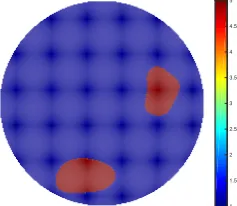
For our iterative method we choose J = 200 ensemble members with regularization parameterρ= 0.8. The covariance of our noiseηis chosen such that Γ = 10−4_{×I. Our} truth for the EIT problem will take the form given in Figure 5 where we have high levels of conductivity within the two inclusions. This is constructed by thresholding a Whittle-Mat´ern Gaussian random field defined by (12), (13); true values for the hierarchical parameters used are shown in Table 1.

Remark 5.1 We do not display the underlying Gaussian random field u which is thresholded to obtain the true conductivity in Figure 5 as this Gaussian random field cannot be expected to be reconstructed accurately, in general. Furthermore it is important to appreciate that in general a true conductivity will not be constructed by such thresholding; the field u is simply an algorithmic construct. We do however show

u, and its evolution, in the algorithm, because this information highlights the roles of the length scale and regularity parameters.

When performing inversion we sample initial ensembles using the prior distributions shown in Table 2. We have set our prior distributions in such a way that the true value for each hyperparameter lies within the range specified.

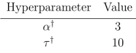
Hyperparameter Value

α† 3

τ† 10

Table 1. Model problem 1. True values for each hyperparameter.

Hyperparameter Prior

α U[1.3,4]

τ U[5,30]

1 1.5 2 2.5 3 3.5 4 4.5 5

Figure 5. Model problem 1: true log-conductivity.

Figure 7. Model problem 1. Progression through iterations of non-hierarchical method with level set.

Figure 9. Model problem 1. Progression through iterations of centered hierarchical method with level set.

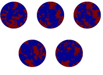
Figure 11. Model problem 1. Progression through iterations of non-centered method with level set.

Iteration

5 10 15 20

τ

5 10 15 20 25 30

Non-hier Centred Non-centred Truth

Iteration

5 10 15 20

α

1 1.5 2 2.5 3

Non-hier Centred Non-centred Truth

Iteration

5 10 15 20

Relative Error

0 0.1 0.2 0.3 0.4 0.5 0.6 0.7

Iteration

5 10 15 20

Log Data Misfit

2 2.5 3 3.5 4 4.5 5 5.5 6

Figure 13. Model problem 1. Left: relative error. Right: log-data misfit.

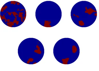
Figure 15. Model problem 1. EKI for the final iteration for the non-centered method with level set from four different initializations.

Figures 6 - 11 show the progression of both the level-set function u, and the permeability κ, through five iterations of the method. Non-hierarchical, centered and non-centered methods are considered in turn. By comparing the reconstructions with the true conductivity, these figures clearly demonstrate two facts: (a) that being hierarchical is necessary to obtain a good reconstruction; (b) that implementing the hierarchical method using a non-centered parameterization has significant benefits when compared to the centered method. These points are further demonstrated in Figures 12 which shows the learning of the hyperparameters, in comparison with the truth, for the three methods.

Concentrating solely on the non-centered approach, we run ten different initializations of the EKI. We display the resulting data-misfit and error, as a function of iteration, for all ten in Figure 13. We display the last iteration of four of these ten in Figures 14 - 15.

5.2. Geometric Parameterization

In this subsection we employ Model Problem 2 from subsection 4.2. We consider reconstruction of a piecewise continuous channel which is defined through two heterogeneous Gaussian random fields, scalar geometric parameters specifying the geometry and scalar hierarchical parameters characterizing the length-scale and regularity of the two fields.

The truth u† is shown in Figure 16. It is drawn from a prior distribution which we now describe; details may be found in [27]. The channel is described by five parameters:

d1– amplitude;d2 – frequency;d3– angle;d4– initial point; andd5– width. We generate two Gaussian random fields {κi}2i=1, both defined on the whole of the domain D but entering the permeability κ only inside and outside (respectively) the channel. The unknown uthus comprises the five scalars{di}5i=1 and the two fields{κi}2i=1.We do not explicitly spell out the mapping fromuto the coefficient κappearing in the Darcy flow, but leave this to the reader. The {κi}2i=1 are specified as log-normal random fields and the underlying Gaussians are of Whittle-Mat´ern type, defined by (12), (13); different uniform distributions on α and τ are used for the two fields {κi}2

i=1 The parameters

{di}5

i=1 are also given uniform distributions. The entire specification of the prior is given in Table 3. For the truth the true hierarchical parameters are provided in Table 4.

In our inversion we employ 64 mollified pointwise observations {li(p)}64i=1 given by, for some σ >0,

lt(p) =

Z

D

1 2πσ2e

− 1 2σ2(x−xt)

2

p(x)dx, (37)

where the xi are uniformly distributed points on D. We discretize the forward model

using a second order centered finite difference method with mesh spacing 10−2_{. For our} EKI method we use the same values for our parameters as in subsection 5.1.

Parameter Prior

d1 U[0,1]

d2 U[2,13]

d3 U[0.4,1]

d4 U[0,1]

d5 U[0.1,0.3]

κ1 N(1,(I−τ12∆)−α1)

κ2 N(4,(I−τ22∆)−α2)

α1 U[1.3,3]

τ1 U[8,30]

α2 U[1.3,3]

τ2 U[8,30]

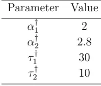
Parameter Value

α†₁ 2

α†₂ 2.8

τ₁† 30

τ₂† 10

Table 4. Model problem 2. Parameter selection of the truth.

0 2 4 6

0 1 2 3 4 5 6

-1 0 1 2 3 4 5

Figure 16. Model problem 2. True log-permeability.

Figure 18. Model problem 2. Progression through iterations of centered hierarchical method.

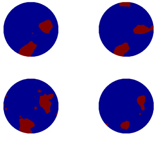
Figure 19. Model problem 2. Progression through iterations of non-centered hierarchical method.

Iteration

5 10 15 20

α 1 1.5 2 2.5 3 Non-hier Centred Non-centred Truth Iteration

5 10 15 20

τ 5 10 15 20 25 30 Non-hier Centred Non-centred Truth

Figure 20. Model problem 2. Progression of average value forα1 andτ1.

Iteration

5 10 15 20

α 1 1.5 2 2.5 3 Non-hier Centred Non-centred Truth Iteration

5 10 15 20

τ 5 10 15 20 25 30 Non-hier Centred Non-centred Truth

Figure 21. Model problem 2. Progression of average value forα2 andτ2.

Iteration

5 10 15 20

Relative Error 0.2 0.3 0.4 0.5 0.6 0.7 0.8 0.9 Iteration

5 10 15 20

Log Data Misfit

2.5 3 3.5 4 4.5 5 5.5 6 6.5 7 7.5 8

methods perform well. We qualify this by noting that the geometry is well-learned in all cases, but that the reconstructions of the random fields u1 and u2 inside and outside the geometry are sensitive to needing non-centered hierarchical representation. Even then the reconstruction is only accurate in terms of amplitude and length scales and not pointwise.

Figures 20 and 21 give further insight into this, showing how the smoothness and length scale parameters are learned differently in the hierarchical, centered and non-centered methods. Again the conclusions are consistent with the previous subsection. Figures 22 and 23 concentrate on the application of the non-centered approach, using ten different initializations. The data misfit and relative error in the field are shown for all ten cases in Figure 22; four solution estimates are displayed in Figure 23. The results are similar to those in the previous subsection. However there is more variability across initializations. This might be ameliorated by use of a larger ensemble size.

5.3. Function-valued Hierarchical Parameterization

Our final set of experiments will be based on hierarchical inversion of non-stationary random fields, using Model Problem 3. We consider reconstruction of truths that are not drawn from the prior; the prior will be a hierarchical Gaussian model with spatially varying inverse length scale as hyperparameter. Examples of such truths are ones which contain both rough and smooth features. We discretize the forward model using a piecewise-linear finite element method (FEM), with a mesh ofh= 1/100. The truth we aim to recover is given by

u†(x) =

               exp

4− 25

x(5−x)

, x∈(0,5)

1, x∈[7,8]

−1, x∈(8,9]

0, otherwise,

(38)

which incorporates both rough and smooth features. Our parameters for the iterative methods are identical to those used in subsection 5.1. Because the results of subsection 5.1 and 5.2 clearly demonstrate the need for non-centring in hierarchical methods, we do not include results for the centered hierarchical approach here; we compare non-hierarchical methods with the use of non-centered hierarchical methods with both Cauchy and Gaussian random fields as priors on the hyperparameter v.

0 2 4 6 8 10

-1 0 1

0 2 4 6 8 10

-1 0 1

EKI Truth

0 2 4 6 8 10

-1 0 1

0 2 4 6 8 10

-1 0 1

0 2 4 6 8 10

-1 0 1

0 2 4 6 8 10 -1

0 1

0 2 4 6 8 10

-1 0 1

EKI Truth

0 2 4 6 8 10

-1 0 1

0 2 4 6 8 10

-1 0 1

0 2 4 6 8 10

-1 0 1

Figure 25. Model problem 3. Progression through iterations with hierarchical Gaussian random field.

0 2 4 6 8 10

-1 0 1

0 2 4 6 8 10

-1 0 1

EKI Truth

0 2 4 6 8 10

-1 0 1

0 2 4 6 8 10

-1 0 1

0 2 4 6 8 10

-1 0 1

Iteration

5 10 15 20

Relative Error 0.2 0.3 0.4 0.5 0.6 0.7 0.8 0.9 1 Gaussian Cauchy Iteration

5 10 15 20

Log Data Misfit

2.5 3 3.5 4 4.5 5 5.5 6 6.5 7 Gaussian Cauchy

Figure 27. Model problem 3. Left: relative error. Right: log-data misfit.

0 2 4 6 8 10 -1

0 1

0 2 4 6 8 10 -1

0 1

0 2 4 6 8 10 -1

0 1

0 2 4 6 8 10 -1

0 1

Figure 28. Model problem 3. EKI for the final iteration for the Gaussian hierarchical method from four different initializations.

0 2 4 6 8 10 -1

0 1

0 2 4 6 8 10 -1

0 1

0 2 4 6 8 10 -1

0 1

0 2 4 6 8 10 -1

0 1

Figure 29. Model problem 3. EKI for the final iteration for the Cauchy hierarchical method from four different initializations.

to initialization may be more significant, as in the previous two subsections.

6. Conclusion & Discussion

In this paper we have considered several forms of parameterizations for EKI. In particular our main contribution has been to highlight the potential for the use of hierarchical techniques from computational statistics, and the use of geometric parameterizations, such as the level set method. Our perspective on EKI is that it forms a derivative free optimizer and we do not evaluate it from the perspective of uncertainty quantification. However the hierarchical and level set ideas are motivated by Bayesian formulations of inverse problems. We have shown that our parameterizations do indeed lead to better reconstructions of the truth on a variety of model problems including groundwater flow, EIT and source inversion. There is very little analysis of EKI, especially in the fixed, small, ensemble size setting where it is most powerful. Existing work in this direction may be found in [7, 48]; it would be of interest to extend these analyses to the parameterizations introduced here. Furthermore, from a practical perspective, it would be interesting to extend the deployment of the methods introduced here to the study of further applications.

Acknowledgements. The authors are grateful to M. M. Dunlop, O. Papaspiliopoulos and G. O. Roberts for helpful discussions about centering and non-centering parameterizations. The research of AMS was partially supported by the EPSRC programme grant EQUIP and by AFOSR Grant FA9550-17-1-0185. LR was supported by the EPSRC programme grant EQUIP. NKC was partially supported by the EPSRC MASDOC Graduate Training Program and by Premier Oil.

References

[1] Aanonsen S I, Naevdal G, Oliver D S, Reynolds A C and Valles B 2009 The Ensemble Kalman Filter in Reservoir Engineering-a ReviewSPE J.14 393-412.

[2] Anderson J L 2001 An ensemble adjustment Kalman filter for data assimilation.Monthly Weather Review 1292884.

[3] Adler A and Lionheart W R B 2006 Uses and abuses of EIDORS: An extensible software base for EIT Physiol Meas 2725-42.

[4] Agapiou S, Bardsley J M, Papaspiliopoulos O and Stuart A M 2014 Analysis of the Gibbs sampler for hierarchical inverse problems.SIAM Journal on Uncertainty Quantification 1511-544. [5] Bakushinsedky A B and Kokurin M Y 2004 Iterative Methods for Approximate Solution of Inverse

ProblemsMathematics and its applications, Springer.

[6] Bauer F, Hohage T and Munk A 2009 Iteratively Regularized Gauss-Newton Method for Nonlinear Inverse Problems with Random NoiseSIAM J. Numer. Anal 471827-1846.

[7] Bl¨omker D, Schillings C and Wacker P 2017 A strongly convergent numerical scheme from EnKF continuum analysis arXiv:1703.06767.

[8] Borcea L 2002 Electrical Impedance TomographyInverse Problems 1899-136.

[10] Burger M and Osher S 2005 A survey on level set methods for inverse problems and optimal design Eur. J. Appl. Math 16263-301.

[11] Carrera J and Neuman S P 1986 Estimation of aquifer parameters under transient and steady state conditions: application to synthetic and field dataWater Resources Research 22228-242. [12] Chada N K 2018 Ensemble Based Methods for Geometric Inverse ProblemsPhD Dissertation. [13] Dashti M Stuart A M 2017 The Bayesian Approach To Inverse ProblemsHandbook of Uncertainty

Quantification 311-428.

[14] Chen V, Dunlop M M, Papaspiliopoulos O and Stuart A M 2017 Robust MCMC Sampling with Non-Gaussian and Hierarchical Priors in High Dimensions,In preparation.

[15] Dunlop M M and Stuart A M 2016 The Bayesian formulation of EITInverse Problems and Imaging

101007-1036.

[16] Dunlop M M, Iglesias M A and Stuart A M 2016 Hierarchical Bayesian Level Set InversionStatistics and Computing.

[17] Emerick A A 2016 Towards a hierarchical parametrisation to address prior uncertainty in ensemble-based data assimilationComputational Geosciences 2035-47.

[18] Ernst, O and Sprungk, B and Starkloff, H. 2015 Analysis of the ensemble and polynomial chaos Kalman filters in Bayesian inverse problems,SIAM-ASA JUQ 3823–851.

[19] Evensen 1994 G Sequential data assimilation with a nonlinear quasi-geostrophic model using Monte Carlo methods to forecast error statisticsJ. Geophysical Research-All Series 9910-10.

[20] Evensen G 2009Data Assimilation: The Ensemble Kalman Filter Springer.

[21] Evensen G and Van Leeuwen P J 1996 Assimilation of geosat altimeter data for the agulhas current using the ensemble Kalman filter with a quasi-geostrophic modelMonthly Weather Review 128

85-96.

[22] Hanke M 1997 A regularizing Levenberg-Marquardt scheme, with applications to inverse groundwater filtration problemsInverse Problems 13 79-95.

[23] Houtekamer P L and Mitchell H L 2001 A sequential ensemble Kalman filter for atmospheric data assimilation Monthly Weather Review 129123-137.

[24] Iglesias M A 2016 A regularising iterative ensemble Kalman method for PDE-constrained inverse problemsInverse Problems 32.

[25] Iglesias M A, Law K J H and Stuart A M 2013 Evaluation of Gaussian approximations for data assimilation in reservoir modelsComputational Geosciences, Volume17851-885.

[26] Iglesias M A, Law K J H and Stuart A M 2014 Ensemble Kalman methods for inverse problems Inverse Problems 29.

[27] Iglesias M A, Lin K, and Stuart A M 2014 Well-posed Bayesian geometric inverse problems arising in subsurface flow 30.

[28] Iglesias M A, Lu Y and Stuart A M 2015 A Bayesian Level Set Method for Geometric Inverse ProblemsInterfaces and Free Boundary Problems.

[29] Kaipo J and Somersalo E 2004 Statistical and Computational Inverse Problems Applied Mathematical Sciences, Springer.

[30] Kalman R E 1960 A new approach to linear filtering and prediction problems Trans ASME (J. Basic Engineering)82 35-45.

[31] Kantas N, Beskos A and Jasra A 2014 Sequential Monte Carlo Methods for High-Dimensional Inverse Problems: A case study for the Navier-Stokes equationsSIAM/ASA J. Uncertain. Quantif

2464-489.

[32] Li G and Reynolds A C 2009 Iterative ensemble Kalman filters for data assimilationSPE J 14

496-505.

[33] Majda A and Wang W 2006Non-linear Dynamics and Statistical Theories for Basic Geophysical Flows Cambridge University Press.

14037-57.

[36] Liang P, Jordan M I and Klein D 2010 Learning Programs: A Hierarchical Bayesian Approach Conference: Proceedings of the 27th International Conference on Machine Learning.

[37] Lindgren F, Rue H and Lindstr¨om J 2011 An explicit link between Gaussian fields and Gaussian Markov random fields: the stochastic partial differential equation approach73423-498.

[38] Liu W, Li J and Marzouk Y M 2017 An approximate empirical Bayesian method for large-scale linear-Gaussian inverse problems arXiv:1705.07646.

[39] Myserth I and Omre H 2010 Hierarchical Ensemble Kalman FilterSPE J 15.

[40] Oliver D, Reynolds A C and Liu N 2008Inverse Theory for Petroleum Reservoir Characterization and History Matching Cambridge University Press.

[41] Papaspiliopoulos O, Roberts G O and Sk¨old M 2003 Non-centered parameterisations for hierarchical models and data augmentation InBayesian Statistics 7: Proceedings of the Seventh Valencia International Meeting. Oxford University Press.

[42] Papaspiliopoulos O, Roberts G O and Sk¨old M 2007 A general framework for the parametrization of hierarchical modelsStatistical Science 59-73.

[43] Pierre Del Moral A J and Doucet A 2006 Sequential Monte Carlo samplersJournal of the Royal Statistical Society Series B 411-436.

[44] Roininen L, Girolami M, Lasanen S and Markkanen M 2017 Hyperpriors for Matrn fields with applications in Bayesian inversion arXiv:1612.02989.

[45] Roininen L, Huttunen J M J and Lasanen S 2014 Whittle-Mat´ern priors for Bayesian statistical inversion with applications in electrical impedance tomographyInverse problems and imaging 8

.561-586.

[46] Ruggeri F, Sawlan Z, Scavino M and Tempone R 2016 A Hierarchical Bayesian Setting for an Inverse Problem in Linear Parabolic PDEs with Noisy Boundary ConditionsBayesian Anal. [47] Santosa, F 1996 A level-set approach for inverse problems involving obstacles ESAIM,

1(January):17–33, 1996.

[48] Schillings C and Stuart A M 2017 Analysis of the ensemble Kalman filter for inverse problems. SIAM J Numerical Analysis55, 1264-1290.

[49] Somersalo E, Cheney M and Isaacson D 1992 Existence and Uniqueness for Electrode Models for Electric Current Computed TomographySIAM J. Appl. Math 52023-1040

[50] Teh Y W, Jordan M I, Beal M J, and Blei D M 2016 Hierarchical Dirichlet processesJournal of the American Statistical Association 1011566-1581.

[51] Tsyrulnikov M and Rakitko A 2016 Hierarchical Bayes Ensemble Kalman Filter Physica D: Nonlinear Phenomena.