Dynamics of globular cluster systems

Dynamics of Globular Cluster Systems

by

Carl

J.

Grillmair

A thesis submitted for the degree of Doctor of Philosophy

of The Australian National University

August, 1992

Mount Stromlo and Siding Spring Observatories

Institute of Advanced Studies

The work described in this thesis is that of the candidate alone , with the following

except ions. Photometry, astrometry, object selection, and design of the aperture

masks used in Chapter 2 were carried out by D. Carter, W. Couch, K. Freeman , and K. Taylor prior to the commencement of this thesis. The globular cluster modeling

discussed in Chapter 3 -was supervised at the California Institute of Technology

by D. Fullagar and J. Salmon. Plates used for star counting in Chapter 4 were taken by the staff of the United Kingdom Schmidt Telescope Unit. Scanning of

these plates was carried out by M. Irwin at the Institute of Astronomy, Cambridge ,

England.

Acknowledgements

It

is with pleasure that I thank Prof. Ken Freeman for having suggested the projects described herein and for having been free with his time and his thoughts. His patience and good humour were always appreciated.

I am also grateful to Dr. Peter Quinn for his guidance and assurances. His personal enthusiasm encouraged me to overcome a variety of setbacks with aplomb. To Dr. Geoff Bicknell , Prof. Agris Kalnajs , and Dr. Jesper Sommer-Larsen I offer my thanks for their advice on several issues and for their occasional lessons in freshman physics.

I am thankful to Prof. Alex Rodgers and the members of several time as-signment committees at Mount Stromlo and Siding Springs Observatories and the Anglo-Australian Telescope for having granted the observing time necessary to carry out the projects described herein.

I gratefully acknowledge the support of Tom Prince and Paul Nlessina, who made it possible for me to run my N-body simulations on the Touchstone Delta. I would also like to offer my heartfelt thanks to John Salmon and David Fullagar for all their labours on my behalf.

I am indebted to the staff of the United Kingdom Schmidt Telescope Unit for their untiring efforts in acquiring the plate material used in Chapter 4. Mike Irwin of the Institute of Astronomy, Cambridge deserves special thanks for single-handedly scanning all these plates with nary a complaint.

I am very grateful to Yong-ik Byun for his friendship and assistance over the years. The efforts of Chris Lidman and Jon Loveday to keep me sound in body, if not in mind, were warmly appreciated. I thank Markus Buchhorn for having allowed me to use his computer for much of the last two years. I am very grateful to all the staff and residents of Mount Stromlo for their patience with my canine prodigy.

As always, I thank my parents and my little sister for their unqualified support over the years.

Abstract

We examine observational aspects of different globular cluster systems to shed

light on possible galaxy formation scenarios. In the first part of this work, we use

low-dispersion spectra of 4 7 globular clusters in the cD elliptical N GC 1399 to

de-termine the velocity dispersion of the cluster system. We find a velocity dispersion

of 388

±

54 km/s, which is significantly higher than the velocity dispersion of the

stellar component of NGC 1399. We see no evidence for a radial gradient in the

dispersion profile though our uncertainties do not impose strong constraints in this

respect. No significant rotation of the globular cluster system is evident. In the

extreme case where the clusters are assumed to be on circular orbits, we determine

a lower limit on a globally-constant mass-luminosity ratio of 79

±

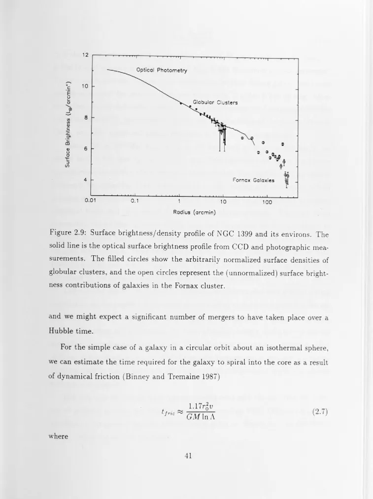
20.

The velocity dispersion of the globular cluster system is very similar to the

unusually low velocity dispersion of galaxies in the Fornax cluster. The surface

density distributions of the stellar light, globular clusters, and Fornax galaxies

follow a similar power-law profile over much of the extent of the cluster.

It

is

unclear whether this has any significance for the formation of the globular cluster

system. M87, the elliptical at the center of the Virgo cluster , has very different

characteristics but its globular cluster system is essentially similar to that of NGC

1399.

We also investigate the dynamics of tidal stripping of globular clusters in a

galactic potential field with a view towards establishing the relationship between

the observed limiting radii of globular clusters in our own Galaxy and their orbit

shapes. We initiate a program of large-scale, self-consistent numerical simulations

to test the validity of the classical King tidal radius under different conditions. Our

simulations, though limited in the amount of parameter space considered, reveal

that slow removal of stars and tidal heating may be responsible for maintaining a

halo of extra-tidal stars which can significantly alter the appearance of the surface

density profile from the profile predicted by the classical King model. Our

simu-lations are not of sufficient duration to determine whether this halo is eventually

removed.

The final portion of this work is aimed at determining accurate limiting radii

for a sample of 12 halo globulars. These clusters are interesting in that their

metal-licities appear to be correlated with their previously inferred orbit shapes. Deep ,

two-colour, photographic photometry is used to select and count stars with colours

and magnitudes consistent with the cluster-specific colour-magnitude sequences.

Owing to the consequent reduction in the number of contaminating foreground

stars, we are able to push the star counts to significantly lower surface densities

Contents

1

Introduction

2

Kinematics of Globular Clusters In NGC

1399

2.1 Introduction.

3

2.2 Observations.

2.3 Velocity Uncertainties.

2.4 Kinematics of the Cluster System ..

2.4.1 Velocity Dispersion.

2.4.2 Radial Velocity Dispersion Profile.

2.4.3 Rotation.

2.5 Globular Cluster Metallicities.

2.6 The Mass of NGC 1399.

2. 7 Discussion.

N-body Modelling of Tidal Stripping

3.1 Introduction.

. . .

3.2 The Parallel N-body Code.

3.3 Initial Model Parameters

3.3.1 The Model Galactic Potential.

3.4 Modelling Results

. . .

3.4·_1 _{Diffusion time scales.}

3.4.2 Response of the Cluster to Truncation.

3.4.3 Results for Orbiting Models.

4 Tidal Radii of Galactic Globular Clusters

4.1 Introduction.

4.2 Observations.

4.3 Star Counts.

4.3.1 Identification of Cluster Stars.

4.3.2 Modelling the Distribution of Field Stars.

4.3.3 Crowding Corrections.

4.4 Limiting Radii. . . . . .

1

5

5

5

29

29

29

32

32

34

36

39

47

47

48

50

55

56

58

67

69

96

96

97

102

102

113

118

149

4.4 .1 Surface Density Profiles .

4.4 .2 Two-Dimensional St ructure.

4.5 Comparison with N-body Simulations.

5 Future Work

References

149

153

173

178

List of Figures

2.1

2.2

2.3

2.4

2.5

Marginal profile of a typical slit.

Template spectra used for cross-correlation analysis.

Sky-subtracted spectra and cross-correlation functions for globular

cluster candidates.

Velocity histrogram for all objects with v

<

3000 km/s.

Velocity dispersion profile of NGC 1399. . . . . .

2.6 _{Cluster velocities as a function of projected distance from the}

rota-tion axis. . . .

2. 7 Composite spectra of metal-rich and metal-poor clusters.

2.8 _{Mass profile of NGC 1399. . . . . .}

8

9

14

31

33

34

35

39

2.9 _{Surface brightness/density profile of NGC 1399 and the Fornax cluster. 41}

3.1 _{Comparison of star count profiles for NGC 1866 with a Jaffe profile. 52}

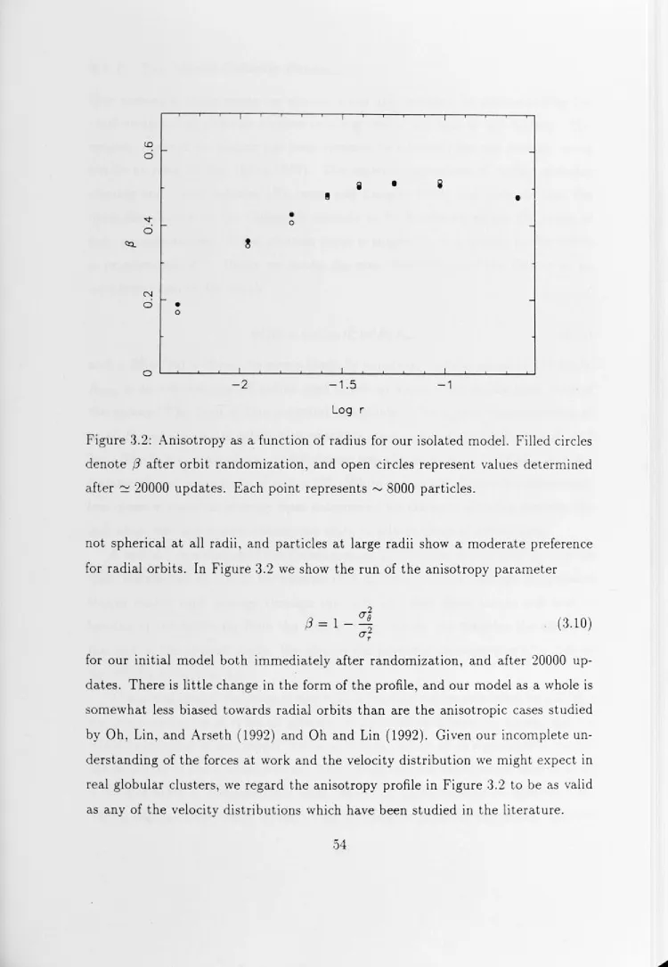
3.2 _{Anisotropy as a function of radius for our isolated model. 54}

3.3 _{Evolution of the mass distribution in our isolated model. 59}

3.4 RMS energy changes with time for an isolated, 32k model evolved

using both single and double precision computations. . . 60

3.5 Velocity distributions in the cores of our 64k and 32k models. 62

3.6 _{RMS, relative energy change as a function of time for our isolated}

32k and 64k models. . . 63

3. 7 Relative change in binding energy over time for individual particles

in our 64k isolated model. . . 64

3.8 _{Observed energy diffusion rates as a function of radius for our}

iso-lated 32k and 64 models. . . 65

3.9 Ratios of observed diffusion rates in our 64k and 32k models. 66

3.10 Time evolution of the density profile of our isolated model after being

stripped of all particles with r

>

3rh. . . . 68

3.11 Radii containing various mass fractions as a function of time for a

3.12 Time evolution of the density profile of our isolated model after being

stripped of all high energy particles. . . 70

3.13 Radii containing various mass fractions as a function of time for an

isolated model stripped of all high energy particles. . . 71

3.14 Volume and surface density profiles of our orbiting 64k models.. 73

3.15 Two-dimensional distribution of particles projected onto the orbit

plane. . . 75

3.16 Two-dimensional distribution of particles immediately surrounding

64eoa as a function of orbital phase. . . 77

3.17 Magnified distribution of particles immediately surrounding 64eoa

as a function of orbital phase. . . 78

3.18 Orbital path of a particle after being stripped from the cluster. . 79

3.19 Velocity dispersion profile for model 64eoa at two points in the orbit. 80

3.20 Velocity dispersion profile for model 64eoc at two points in the orbit. 81

3.21 Successive density profiles for model 64eoa during the sixth

peri-galactic passage. . . ₈₂

3.22 Fraction of cluster mass lost over time. 84

3.23 Density of particles beyond rt as a function of the number of orbits. 85

3.24 Anisotropy as a function of time in the outskirts of our model clusters. 86

3.25 Energy and angular momentum per unit mass for particles lost from

model 64eoa. . . 87

3.26 Energy and angular momentum per unit mass for particles lost from

model 64eoc. . . 88

3.27 Fraction of particles on prograde orbits as a function of radius. 89

3.28 Mean z-component of angular momentum per unit mass and the

relative fraction of particles on prograde orbits as a function of time. 90

3.29 Time evolution of the radii containing various mass fractions for

model 64eoa. . . 91

3.30 Mean square change between successive updates in the z component

of angular momentum relative to the mean square change in total

angular momentum. . . . 93

4.2 Contour map of the colour-magnitude distribution of stars in NGC

3201 . . . 111 4.3 . Cumulative star-count, signal-to-noise ratio as a function of enclosed

colour-magnitude area for NGC 362. . . . . 113 4.4 Comparison of 1st and 2nd-order surface fits to the foreground

dis-tributions surrounding NGC 3201. . . 115 4.5 Comparison of 1st and 3rd-order surface fits to the foreground

dis-tribution surrounding NGC 7089. . . . 116

4.6 Software reseau used for star counting. 118

4. 7 Ratio of bright stars to faint stars as a function of radius in a

rep-resentative selection of sample clusters. . . 121 4.8 Ratio of bright stars to faint stars as a function of total surface

density in a representative selection of sample clusters. . . 122 4.9 Contributions to the total surface density by different classes of images.123 4.10 Surface density profiles of sample clusters. . . . . f36 4.11 Residuals after subtraction of King models from the surface density

data. . . 1.so 4.12 Contour maps of the background-subtracted surface density

distri-butions. . . 1.55 4.13 Colour-magnitude distribution of images extending westwards from

NGC 6864 . . . 170 4.14 Two-point correlation function for stellar and non-stellar images

sur-rounding NGC 7089 . . . 172 4.15 Comparison of the foreground-subtracted surface densities of

non-stellar images with those of non-stellar images for the field surrounding

NGC 7089 . . . 174 4.16 Smoothed, 2-dimensional distribution of particles in model 64eoc as

it would appear from a distance of 12 kpc. . . 176 4.17 Comparison between the surface density profiles of NGC 7089 and

List of Tables

2.1 Observing Log. . . . .

2.2 Cross-correlation Results.

2.3 Velocity Dispersion Results.

3.1 Model Orbit Parameters

4.1 Basic Cluster Data. . .

4.2 Observational Details.

4.3 Sources of Surface Density Data.

4.4 NGC 288 Star Counts.

4.5 NGC 362 Star Counts.

4.6 NGC 1904 Star Counts.

4. 7 NGC 2808 Star Counts.

4.8 NGC 3201 Star Counts.

4.9 NGC 4590 Star Counts.

4.10 NGC 5824 Star Counts.

4.11 NGC 6864 Star Counts.

4.12 NGC 6934 Star Counts.

4.13 NGC 6981 Star Counts.

4.14 NGC 7078 Star Counts.

4.15 NGC 7089 Star Counts.

4.16 Fitted Tidal Radii . . . .

6

11 30

57

Chapter

1

Introduction

Globular clusters are among the oldest known objects in the Universe. While they

are fascinating physical entities in their own right, they may also bear the fossil

imprint of processes which led to the formation of galaxies. The orbits of globular

clusters which do not penetrate the dense, central regions of galaxies will not have

been altered significantly since the final stages of galactic collapse. The structure

and kinematics of globular cluster systems thus provide us with an excellent tool with which to study both the present structure of galaxies as well as the dynamics

of galaxy formation.

Globular clusters are intrinsically luminous (lvlv ~ -7.8) and have been de-tected out to distances of order 50 Mpc. At these distances they appear as

collec-tions of unresolved point-sources concentrated towards the centers of galaxies. The

number of known globular cluster systems has increased steadily with the advent of

larger telescopes and more efficient detectors. With the introduction of multi-slit

spectrographs, it has recently become possible to obtain kinematic data for

glob-ular cluster systems at moderately large distances (Mould, Oke, and Nemec 1987;

Huchra and Brodie 1987; Mould et al. 1989).

Excellent reviews on the subject of extragalactic globular cluster systems have

been given by Harris and Racine (1979), Harris (1986), and Harris (1991), and the

reader is referred to these works for an overview of the field. Of particular interest

are the "superabundant" globular cluster systems surrounding several cD ellipticals.

In Chapter 2 we examine the kinematics of the globular cluster system of NGC

1399, the cD galaxy at the center of the Fornax cluster. This galaxy has attributes

similar to those of several other cD ellipticals, including a very extended stellar

envelope (Schombert 1986), an even more extended X-ray emitting region (Thomas

et al. 1986; Killeen et al. _{1988), and a very large population of globular clusters}

(Hanes and Harris 1986; Bridges et al. 1991). As in the case of M87 (Fabricant

et al. _{1980), the virial temperature of the X-ray emitting gas has been found to be}

a

this has important implications for the amount of dark mat ter surrounding CC

1399, the uncertainties associated with the X-ray data are large. \,Vith the aim of

putting better constraints on the form of the potential at intermediate radii , we

have undertaken to measure the velocity dispersion of the globular cluster system

surrounding NGC 1399. We find that the kinetic temperature of the cluster system

is significantly higher than that of the stellar component nearer the core , but is in

good agreement with the X-ray observations. This implies that the mass-luminosity

ratio must increase by almost an order of magnitude between 5 and 20 kpc from

the center. The structure and kinematics of the globular cluster system appears

to have many features in common with the cluster system of M87 (Harris 1986;

Mould et al. 1989), reaffirming the view that globular cluster systems are far more similar to one another than are their parent galaxies.

The use of globular clusters to determine the structure of our own Galaxy goes

back to Harlow Shapley's determination of the center of the Galaxy using the their

apparent distribution in space (Shapley 1918). Since then, globular clusters have

become a cornerstone for our understanding of the age, structure, and dynamics

of the Galaxy. The literature is vast, and we refer the reader to Harris and Racine

(1979) and Freeman and Norris (1981) for guidance. In Chapters 3 and 4 we study

effects of the Galactic tidal field on the apparent diameters of globular clusters

and attempt to improve on published determinations of this quantity. This study

was originally motivated by the curious finding of Seitzer (1983) (see also Freeman

and Norris 1981) that the metallicities of clusters appeared to be correlated with

the orbital radii at perigalacticon; clusters whose orbits take them nearer to the

Galactic center generally have higher metallicities. Such a correlation is not nearly

as evident in a plot of metallicity against present Galactocentric distance , and one

possible inference is that clusters may have actually formed near their perigalactica

( Freeman and Norris 1981)

Frenk and White ( 1980) used radial velocities of globular clusters to establish

that their velocity distribution is approximately isotropic. Based on the postulates

that globular clusters are limited in extent by the Galactic tidal field, and that

the limiting radii are established at the perigalactic points of cluster orbits ( von

Hoerner 1957; King 1962), Peterson (1974) attempted to put constraints on t he

shapes of globular cluster orbits using the published values for the King tidal radius ,

rt (King 1966). The results of this work were not entirely credible since the inferred perigalactic distances for several clusters were found to be greater than their present

galactocentric distances. Innanen, Harris, and Webbink (1983) carried out a similar

study and concluded that globular cluster orbits were rather more circular than an

isotropic velocity distribution would suggest. However, their attempts to determine

individual cluster perigalactica were defeated, and they cited the large uncertainties

in published values of rt as being responsible.

One important factor which affects the determination of a globular cluster's

minimum orbital radius is the relationship between the value of rt inferred from observed surface density profiles and the Galactic tidal field. King ( 1966) developed

his now-famous model for globular clusters based on a distribution function which

incorporated a binding energy cutoff. This cutoff he ascribed to the removal of

loosely bound stars by externally-imposed tidal stresses. Since then, the King

model has been found to be remarkably successful in matching both the observed

structure ( over several decades in surface density) and velocity dispersions of a

substantial number of Galactic globular clusters. What makes the King model

particularly attractive is that it requires what amounts to the minimum number of

parameters to describe a given system, these being (

i)

the total number of stars, ( ii) the total energy of the system, and ( iii) the strength of the imposed tidal field.

King models have been successfully used to model clusters of galaxies as well.

Globular cluster evolution and the process of tidal stripping have been addressed

many times both analytically ( e.g. Chandrasekhar 1942; von Hoerner 1957; King 1962; Jeffreys 1974; Innanen, Harris, and Webbink 1983) and numerically ( e.g. Jef-freys 1974, 1976; Keenan and Innanen 1975; Keenan 198la,b; Seitzer 1983; Lee

and Ostriker 1987; Allen and Richstone 1988; McGlynn 1990; McGlynn and Borne

1991). Many works have focussed on the the stability of various types of stellar

orbits under the influence of tidal forces, and the consensus is that the short-term

effects of tidal processes on clusters are considerably more complicated than the

simple binding energy cutoff inherent in King models. The question of whether rt

accurately predicts the eventual limiting radii of clusters is still a source of some

To date , no large- scale , self-consis tent si mulations of tid al stripping have been

carried out owing to hardware limitations. In Chap t er 3 we describe initial resul ts

of an ongoing project to model the evolution of a 64000-particle cluster orbiting in

an isothermal potential field. Simulations on this scale are made possible by the

recent advent of parallel computer architectures and more efficient N-body codes

(Sellwood 1987). To date we have evolved a single cluster model along several

eccentric orbits for the equivalent of 2 x 109 years. The results generally agree with

the work of previous investigators, though we cannot yet make firm conclusions

concerning the validity of rt,

In Chapter 4 we address the problem of refining the observed limiting radii of

globular clusters. Published values of rt are determined by fitting King models to the surface density profiles (see Elson, Hut, and Inagaki, 1987, and references

therein). These profiles are usually constructed from aperture photometry near

the cluster center and star counts at large radii where the surface density is low.

At some finite radius, the star counts are overwhelmed by the surface density · of

foreground stars, and the limiting radii of globular clusters have never actually

been seen. In the expectation that the fitted values of rt could be improved by removing a substantial fraction of the foreground stars and extending the star

counts to larger radii, we have carried out star counts of a sample of 12 halo

clusters. Using 2-colour photometry from sky-limited, photographic plates, we are

able to remove as much as 90% of the foreground stars from the counts. The results

are somewhat of a surprise in that many of the clusters for which we have high

quality data show significant departures from King-like behaviour. The departures

are consistent in several respects with the results of Chapter 3, and we identify the

extra-tidal material with stars which are still in the process of leaving the cluster.

Unfortunately, this effectively robs us of our hoped-for ability to refine existing

determinations of rt.

This work is necessarily incomplete and in Chapter 5 we briefly describe

contin-uing and follow-up work which may resolve some of the issues raised in the following

Chapter

2

Kinematics of Globular Clusters In NGC

1399

2.1

Introduction.

NGC 1399 has recently been the subject of considerably scrutiny 1n the optical (Killeen and Bicknell 1988, hereafter KB; Bicknell et al. 1989, hereafter BCKB),

radio (Killeen et al. _{1988), and X-ray wavelengths (Mason and Rosen 198.S; Thomas}

et al. _{1986, KB). This investigation has been primarily motivated by the finding of}

KB that the X~ray-emitting gas surrounding NGC 1399 has a virial temperature at least twice that of the stellar component. Fortuitously, NGC 1399 is among several known cD galaxies with "superabundant" globular cluster systems and is estimated to contain of order 15000 clusters. Their intrinsic luminosities make globular clusters visible out to~ 20 Mpc and hence suitable for tracing the potential field of NGC 1399 in the region where the integrated stellar light becomes too faint to yield useful information. The high concentration of globular clusters in this region and recent advances in efficient multi-slit spectrographs make this an ideal starting point in any efforts to reconcile the X-ray and optical measurements made to date.

In Section 2.2 we _{summarize our observations and reduction proced ll res.}

Veloc-ity uncertainties are discussed in Section 2.3. Section 2.4 describes the kinematics of the cluster system, and metallicity of the clusters is discussed in Section 2.5. A lower limit on the mass required to contain the globular cluster systcrn is deter-mined in Section 2.6. Finally, in Section 2.7 we consider the implications of our results for likely formation scenarios.

2.2

Observations.

The objects we have chosen to study were selected from B and R photometry of deep IIIaJ and IIIaF plates in the Anglo-Australian Telescope archi \·e. The plates were scanned on a PDS machine by W. Couch and the results \Vere calibrated

Date

October 13, 1988 October 14, 1988 October 15, 1988 November 27, 1989 November 28, 1989 November 29, 1989 November 29, 1989

Table 2.1: Observing Log.

Field Total Integration Time (seconds)

Core 17500

East 12000

East 18800

West 20400

East 22032

West 9000

Core 7565

Average Seeing ( arcseconds)

1.0 3.0 3.0 2.5 1.5 1.2 3.0

Only objects within 9' of the core of NGC 1399 were considered owing to Jhe

rapidly increasing proportion of contaminating foreground stars beyond this radius.

Red objects were rejected to further reduce contamination, and our final sample

included objects which satisfied 21

<

B

<

22.5 and 0. 7

<

B - R

<

1.4.

Spectroscopy of these objects was carried out during two observing seasons

using the multi-slit Low-Dispersion Survey Spectrograph (LDSS) on the

Anglo-Australian Telescope. The LDSS is described at length by Wynne and Worswick

(1988) and Colless

et al.

(19.90). In the high-dispersion mode, the LDSS has a

point-spread-function with FWHM "' 13A. Three aperture masks were

manufac-tured to sample candidate objects in three overlapping fields centered on N GC

1399. To make maximum use of the 5' x 12' field area available on the Image

Photon Counting System (IPCS) detector, we used a filter to effectively remove

all light redward of 4800

A.

Slit lengths were optimized to gain as much sky

in-formation as possible; a total of between 34 and 38 slits were etched into each of

the three masks. A 2' overlap between adjoining fields allowed us to make

multi-. ple observations of selected targets as an aid in estimating our uncertaintiesmulti-. Our

spectroscopic observations are summarized in Table 2.1.

Our reduction procedures are essentially identical to those of Colless

et al.

100 second exposures of a copper-helium arc lamp. Spatial and wavelength shifts

between exposures taken on the same night were found to be minimal ( typically

less than 0.1 pixels), so individual exposures were coadded to improve the

signal-to-noise ratio. Arc calibration was carried out using 5 unblended arc lines and

wavelength calibration coefficients were computed using 3rd order polynomial fits.

The

RMS

residuals between the calibrated wavelengths and the centroids of the

arc lines were typically 0.3

A.

The slits etched into the aperture masks were not perfectly uniform , usually

being slightly wider at the ends than in the middle. A correct estimate of the sky

level ( which could be as much as ten times higher than that of the target object )

re.-quired that we carefully correct for both this nonuniformity and the gradient in the

luminosity profile of NGC 1399. The marginal profile of each slit was determined

by compressing the entire spectral image along the wavelength coordinate. The

sky level at the spatial position of the object was determined by fitting a low order

polynomial to the marginal profile, or where necessary, estimating the sky level

by eye. The resulting spatial surface brightness profile was normalized to unity

and divided into each wavelength column. Regions of the spectral image were then

selected to avoid other discrete sources in the slit, and the sky level was determined

by averaging over these regions. A typical ex?1,mple of a marginal profile is shown

in Figure 2.1.

Our final, co-added spectra were cross-correlated with a variety of template

spectra using standard cross-correlation techniques (Tonry and Davis 1979). vVe

used as templates high signal-to-noise ratio, integrated cluster spectra of NGC 7078,

NGC 7089, NGC 2808, and 47 Tue. In addition, we used a composite spectrum of

six globular clusters in the Fornax dwarf spheroidal, an integrated spectrum of the

metal-weak, Fornax dwarf elliptical G- 79, and a composite K-giant spectrum. We

are grateful to M. Winsall, M. Gregg, and J. Sommer-Larsen for providing us with these spectra. The smoothed template spectra are shown in Figure 2.2.

All spectra were logarithmically binned into 256, 330 km/s channels , and the

bluemost and redmost 5% of the spectra were cosbelled to zero. Cross-correlations

were carried out in Fourier space, and low frequency components in the final

ti)

_,

C

::::,

0

u

0

_,

•

0 _...

X

I/)

N

•

0

...

X "St

N

o,.

I- 0

...

X

t0 N

•

0 _...

X

N N

0

overlapping

,lit

,Icy

10

point source

sky

20

L...J

target object

Row Number

Object 25

extended source

30

sky

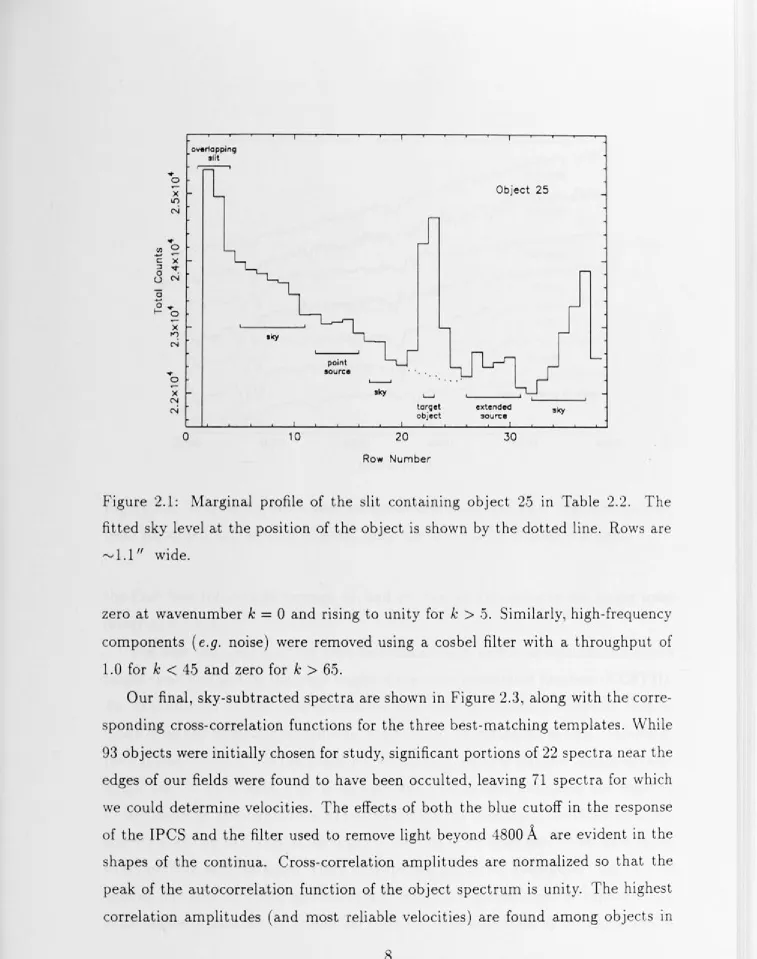
Figure 2.1: Marginal profile of the slit containing object 25 in Table 2.2. The

fitted sky level at the position of the object is shown by the dotted line. Rows are

""1.1" wide.

zero at wavenumber

k

=

0 and rising to unity for

k

>

5. Similarly, high-frequency

components ( e.g. noise) were removed using a cosbel filter with a throughput of

1.0 for

k

<

45 and zero for

k

>

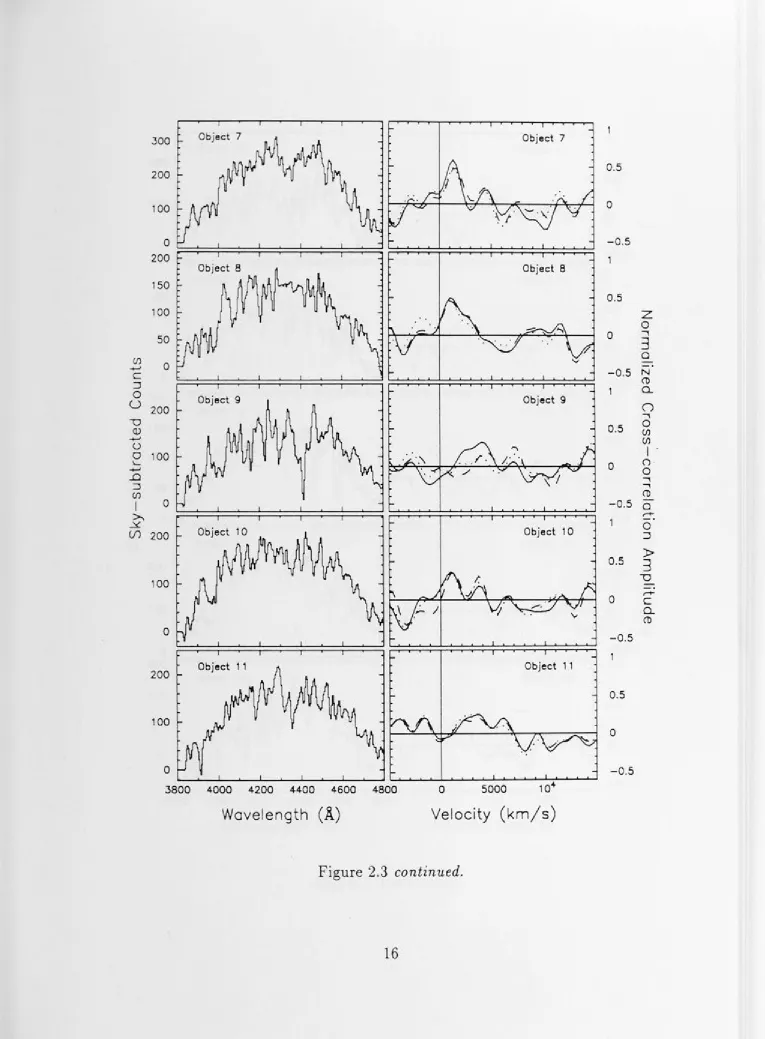
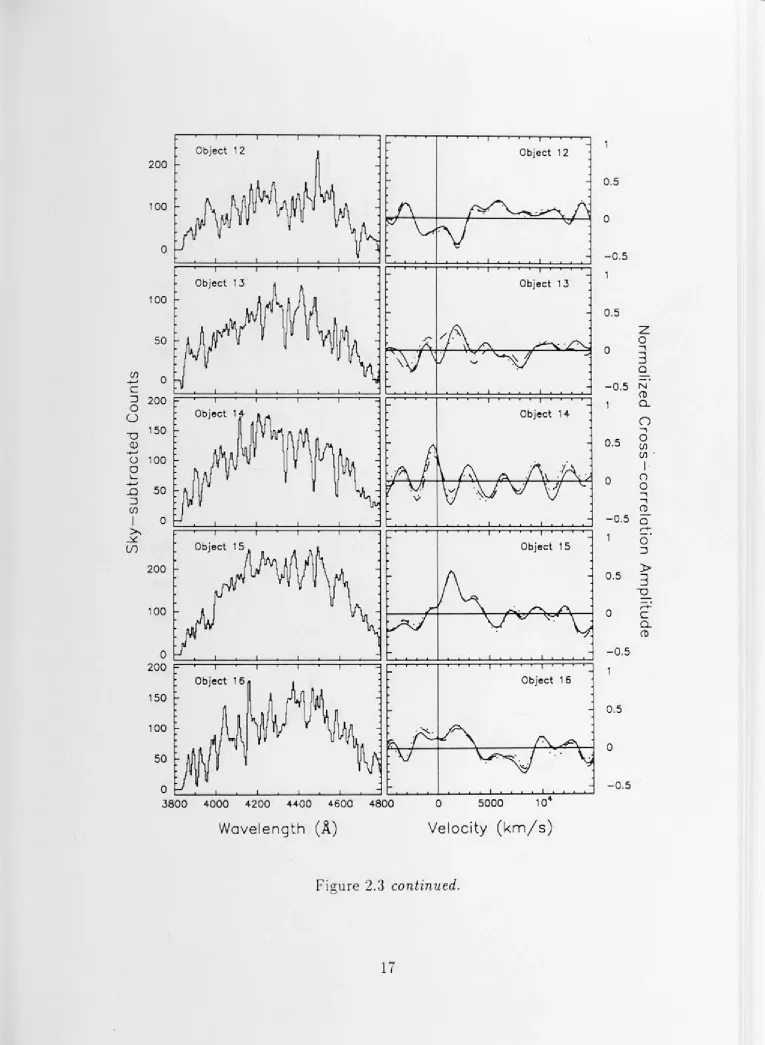
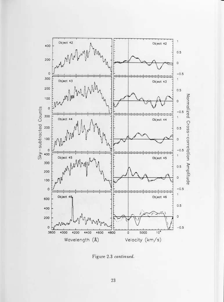
65.

Our final, sky-subtracted spectra are shown in Figure 2.3, along with the

corre-sponding cross-correlation functions for the three best-matching templates. While

93 objects were initially chosen for study, significant portions of 22 spectra near the

edges of our fields were found to have been occulted, leaving 71 spectra for which

we could determine velocities. The effects of both the blue cutoff in the response

of the IPCS and the filter used to remove light beyond 4800

A

are evident in the

shapes of the continua. Cross-correlation amplitudes are normalized so that the

peak of the autocorrelation function of the object spectrum is unity. The highest

[image:20.798.22.779.29.988.2]

F'ornox Globular Clusters

3800 4000 4200 4400 4600 4800

Wavelength (A)

Figure 2.2: Template spectra used for cross-correlation analysis. The spectra have

been smoothed and arbitrarily offset from one another for display purposes.

the East field (objects 39 through 41, and 49 through 71) owing to the longer total

integration time.

The best template matches were determined both by visual examination of the

target spectrum and by the peak height of the cross-correlation function (CCFPH).

An examination of the cross-correlation functions in Figure 2.3 reveals that in

many cases the peaks are asymn1etric and marginally significant at best. Moreover ,

poor sky-subtraction is occasionally responsible for spurious features of considerable

amplitude. In such cases. individual correlation peaks were evaluated and rejected

if they could be at tri bu ted only to features in the sky spectrum. Artificial template

spectra made up of Gaussian absorption features of variable line ratios were found

to be useful in such instances . Once the expected pattern of absorption lines beating

against one another could be established, spurious features could be rejected with

to the relevant peaks in the cross-correlation functions. The final velocity was

taken as a mean of velocities determined using the three best-matching templates.

Spectra were classed as Galactic halo stars if their velocities were less than 400 km / s

and as globular clusters if 400 km/s

<

v

<

3000 km/s. Objects with v

>

3000 km/s or with spectra having obvious emission features were classified as background

galaxies. The velocities for these objects are generally quite unreliable owing to

mismatch between the template and object spectra. The positions , magnitudes ,

Table 2.2: Cross-correlation Results.

ID# a 8 BJ BJ - R V CCFPH

(1950 ) ( 1950) (km/s )

1 03 35 47.3 -35 40 21 21.7 1.31 1121 0.45

2 03 35 47.2 -35 35 33 21.8 0.86 4666 0.30

3 03 35 47.5 -35 39 54 21.6 0.90 3331 0.28

4 03 35 49.2 -35 36 44 22.3 1.04 2478 0.39

5 03 35 50.1 -35 38 48 21.3 1.32 1624 0.75

6 03 35 51.4 -35 37 52 21.9 1.13 1186 0.41

7 03 35 ,52.0 -35 32 44 21.5 0.98 1385 0.52

8 03 35 54.8 -35 38 09 22.4 0.84 1152 0.47

9 03 35 56.2 -35 37 17 22.1 1.07 ,.__,4000

10 03 35 58.4 -35 36 03 21.9 0.91 1068 0.36

11 03 36 02.0 -35 41 37 21.7 1.00 3258 0.23

12 03 36 02.1 -35 35 06 22.0 0.91 ,.__,5000

13 03 36 03.6 -35 31 58 21.9 1.05 1922 0.29

14 03 36 03.9 -35 33 39 22.1 1.31 -381 0.41

15 03 36 05.2 -35 39 54 21.7 1.05 1355 0.56

16 03 36 05.9 -35 34 20 22.1 1.16 1766 0.29

17 03 36 07.8 -35 34 44 22.3 0.89 1784 0.27

18 03 36 11.2 -35 32 34 22.4 1.08 ,.__,5000

19 03 36 17.0 -35 36 46 21.6 1.52 ,.__, 15000

20 033617.8 -35 38 42 21.6 1.33 1836 0.67

21 03 36 18.2 -35 40 52 21.9 1.27 2085 0.37

22 03 36 19.0 -35 39 29 21.7 1.26 3844 0.41

23 03 36 20.3 -35 35 15 22.4 1.06 1761 0.32

24 03 36 21.5 -35 36 04 21.4 1.50 980 0.71

25 03 36 22.7 -35 38 12 22.4 1.19 2182 0.37

26 03 36 23.5 -35 37 25 21.8 1.54 1646 0.53

27 03 36 14.7 -35 33 54 22.3 0.81 1921 0.37

28 03 36 16.7 -35 37 02 21.7 1.31 1677 0.37

29 03 36 19.2 -35 36 29 21.8 1.33 1280 0.58

ID# a

( 1950)

31 03 36 24.7

32 03 36 29.6

33 03 36 30.1

34 03 36 35.1

35 03 36 35.7

36 03 36 41.3

37 03 36 42.8

38 03 36 43.0

39 03 36 44.5

40 03 36 44.4

41 03 36 45.7

42 03 36 45.8

43 03 36 46.0

44 03 36 48.7

45 03 36 50.9

46 03 36 51.8

47 03 36 51. 7

48 03 36 52.4

49 03 36 46.9

50 03 36 48.5

51 03 36 48.7

52 03 36 51.8

53 03 36 51. 7

54 03 36 51.9

55 03 36 54.0

56 03 36 54. l

57 03 36 55.4

58 03 36 59.3

59 03 36 .59.9 60 03 36 ,59.9

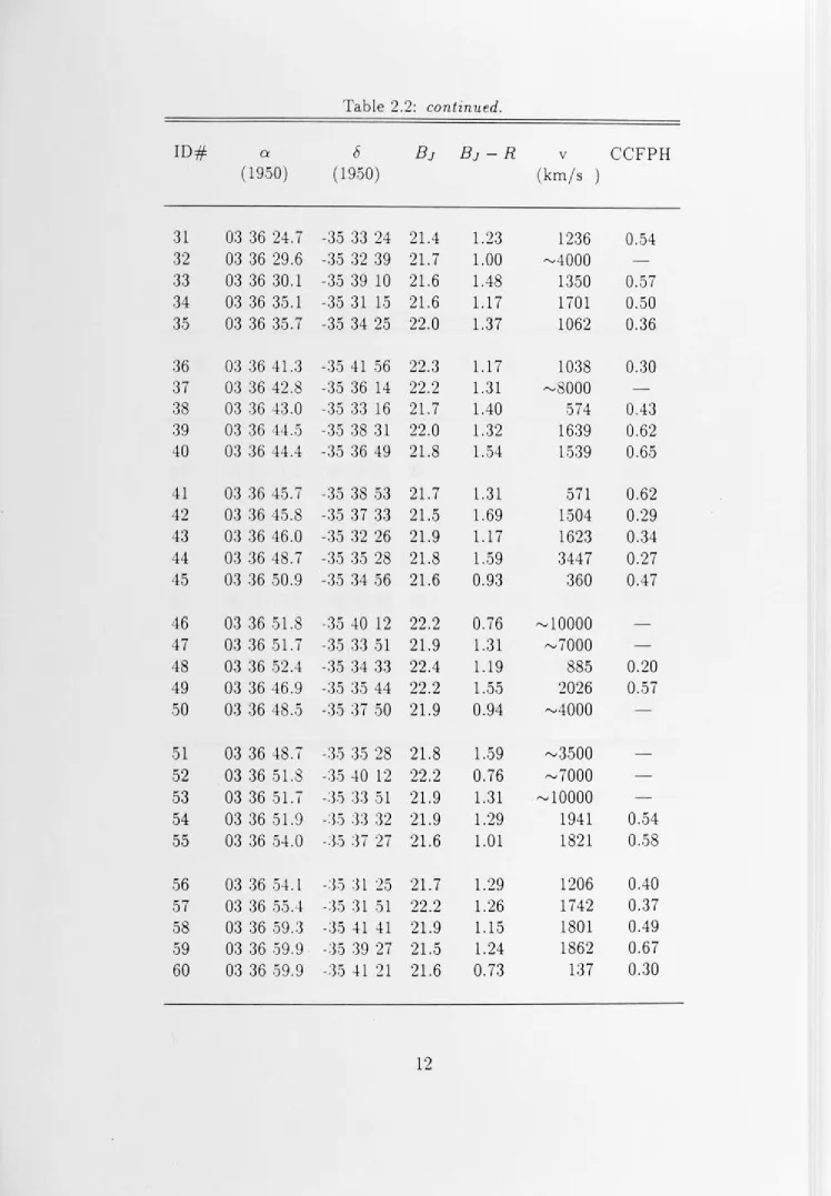
Table 2.2: continued.

8

(1950)

BJ BJ - R V CCFPH

(km/s )

-35 33 24 21.4 1.23 1236 0.54

-35 32 39 21.7 1.00 rv4000

-35 39 10 21.6 1.48 1350 0.57

-35 31 15 21.6 1.17 1701 0.50

-35 34 25 22.0 1.37 1062 0.36

-35 41 56 22.3 1.17 1038 0.30

-35 36 14 22.2 1.31 rv8000

-35 33 16 21.7 1.40 574 0.43

-35 38 31 22.0 1.32 1639 0.62

-35 36 49 21.8 1.54 1539 0.65

-35 38 53 21.7 1.31 571 0.62

-35 37 33 21.5 1.69 1504 0.29

-35 32 26 21.9 1.17 1623 0.34

-35 35 28 21.8 1.59 3447 0.27

-35 34 56 21.6 0.93 360 0.47

-35 40 12 22.2 0.76 ""'10000 -35 33 51 21.9 1.31 ""'7000

-35 34 33 22.4 1.19 885 0.20

-35 35 44 22.2 1.55 2026 0.57

-35 37 50 21.9 0.94 rv4000

-3.5 35 28 21.8 1.59 rv3500

-:3.5 40 12 22.2 0.76 rv700Q

-J.5 33 51 21.9 1.31 ""'10000

-:3.S :3:3 32 21.9 1.29 1941 0.54

-:3.5 :37 27 21.6 1.01 1821 0.58

-:J,5 31 25 21.7 1.29 1206 0.40

-:35 31 ,51 22.2 1.26 1742 0.37

-:35 41 41 21.9 1.15 1801 0.49

-:3.5 39 27 21.5 1.24 1862 0.67

[image:24.798.31.779.26.1103.2]

Table 2.2: continued.

ID# a

8

B1 BJ - R V

CCFPH

( 1950) ( 1950)

(km/s )

61 03 37 01.1 -35 40 49 21.9 0.95 157 0.37

62 03 37 01.2 -35 34 32 21.2 1.35 794 0.73

63 03 37 02.2 -35 38 16 21.8 0.82 1282 0.43

64 03 37 06.6 -35 33 14 21.3 0.80 -42 0.68

65 03 37 09.1 -35 32 42 21.1 1.24 67 0.83

66 03 37 10.1 -35 36 36 21.8 0.98 845 0.68

67 03 37 10.8 -35 38 42 22.3 1.09 1343 0.39

68 03 37 14.3 -35 37 11 21.6 1.18 1166 0.57

69 03 37 15.1 -35 33 46 22.4 0.97 1938 0.34

70 033717.3 -35 35 38 22.3 0.98 ,.._,5000

(J) +-'

§ 300 Object 1

0

u

--0 200

Q)

+-'

u 0

L. +-' 100 ...0

::J

(J) I

~ 0

.:x.

(J)

3800 4000 4200 4400 4600 4800

Wavelength

(X)

Object 1

0 5000 104

Velocity (km/s)

0.5

0

0 """"I

0

CJ) CJ) I

0

0

""""I """"I (1)

0

,-+

0

::J

)> .

3·

--0

-0 .5 ,_

C

0... (1)

Figure 2.3: Sky-subtracted spectra and normalized cross-correlation functions for

all objects listed in Table 2.2. C ross-correlation functions are shown only for the

Obj ect 2 _{Obj ect 2}

200

100

0

300 Obj ect 3 Object 3

200

100

(j) -+--'

C 0

::J

::==:::=~===::::=:::=~===::::=:::=~===::::=~

~~~~~~=;::::;:::!=;::::;=::=::::;::::~~

0

U 200

~ 150

-+--'

0

O 100

L

-+--'

Ll 50

::J (/)

Object 4 Object 4

~ o::=::!:=::::;:~=::!==:::==:=:!=::=======;::;:~~~~::=::::!=:!:=!=!=~=!=:;:::;~

~ 400

300 200 100 200 100 0

Object 5

Object 6

3800 4000 4200 4400 4600 4800

Wavelength

(A)

Object 5

Object 6

0 5000 10~

Velocity (km/s)

Figure 2.3 continued.

0.5 0 -0 .5 0.5

z

0

0 -,

3 Q

-0.5 N

(1) 0 .5 0 0.. 0 -, 0 Cl) Cl)

-I_

(")

0 _-,

-,

(1)

-0.5 o

300 200 100 150 100 50

2

0

C

::J

0

U 200

-0

Q)

+-'

u

0 100

..._

-+-'

..0

::J

CJ)

Obj ect 7 Obj ect 7

Ob j ect 8

Object 9 Object 9

I o

>, :::=:::::::==::==:::::::::::===::==~=:::==::==:!=~ :=~~~~~~~~~~~~~ ..:::£.

(/) 200 Object 10

100

0

200 Object 11 Object 11

100

0

3800 4000 4200 4400 4600 4800 0 5000 10~

Wavelength (.~) Velocity (km/s)

Figure 2.3 continued.

0.5 0 -0 .5 0.5

z

0 0 -,

3

0

-0.5 N

(1) 0.5 0 a. 0 -, 0 CJ) CJ)

I .

()

-0 _-,

-,

(t) -0.5 o

[image:28.796.17.782.23.1062.2]

200

100

0

100

50

2

0

C

::, 200

0

u

-0 Q) -+-' u 0 ..._ -+-' ..0 :J (J) I >, ..Y. (/) 150 100 50 200 100 150 100 50

Ob j ect 12 _{Obj ect 12}

Object 13 Obj ect 13

Object 14

Object 15

Object 16 Object 16

0 .__..._.___.__...___.i..._...__....J...___.__..____._--' i....i... ... ~ ... ....__.__._..,___..._...___._...,,...__,_ ...

3aoo 4000 4200 4400 4600 4800 o 5000 1 o4

Wavelength

(A)

Velocity (km/s)

Figure 2.3 continued.

0.5 0 -0 .5 0.5

z

0 0 ....,

3

a -0.5 N

(t) 0.5 0 a.. 0 ...., 0 (/) (/) . l-o 0 ...., ...., (t)

-0.5 a

[image:29.796.17.782.20.1065.2]

(/) +-' 100 50 0 150 100 50

Object 17 _{Ob j ect 17}

Object 18 Object 18

§ 0 ~=!==;:==;=::::::;::=;:==!:==!==::::==::==~~~:;::::;~~=;:::!=!=;::;:::!=:::;:::!~~

O 800

u

600 400 200 600 400 200

Object 19 Ob j ect 19

Object 20 Object 20

0 ::=:::=:::;::==!:=:!=::!:=:=;:==!=:!::::=::::!===! :=;:::;:::;:::;:=:;::~:::;:::;::::;::;::;:::;:~:=:;::~~

400

300

200

100

0

Object 21

C....-'---'--"""---'--'---l-__.,_..1..--__._-.2

3800 4000 4200 4400 4600 4800

Wavelength

(A.)

Object 21

0 5000 10~

Velocity (km/s)

Figure 2.3 continued.

0.5 0 -0 .5 0.5 0

z

0 -, 3 0

-0 .5 N

(1) 0.5 0 -0 .5 0.5 0 -0 .5 0.5 0 -0 .5 Q. 0 -, 0 (fJ (fJ .

(J) -+--' C :J 800 600 400 200 0 300 200 100 0

Object 22 _{Object 22}

Object 23 _{Object 23}

81000 Object 24 _{Object 24}

-0 Q) -+--' u 0 I.... -+--' ..0 :J (/) I >, _y U) 500 400 200 0 800 600 400 200

Object 25 Object 25

~~~==:=::::!===!:==:;:=:::::!===!:==:;:=::::::!

Object 26 Object 26

0 ,..__....____.__...____,___.__ ____ ___.__...___._~ I...J...J... ... ...__ ... ...,..._._ ...

3aoo 4000 4200 4400 4600 4aoo o 5000 1 o4

Wave length (~) Velocity (km/s)

Figure 2.3 continued.

0.5 0 -0 .5 0.5

z

0

0 -,

3

a

-0.5 N

(1) 0.5 0 -0 .5 0.5 0 -0.5 0.5 0 -0.5 a. 0 -, 0 (/) CJ)

150

100

50

0

300

200

100

100

0

400

200

0

Object 27 _{Object 27}

Object 28 _{Object 28}

Object 29 _{Object 29}

Object 30 _{Object 30}

Object 31 Object 31

.._...___.._...____.__...__...____.__.._____._____.

3800 4000 4200 4400 4600 4800 0 5000

Wavelength

_(ll)

_{Velocity (km/s)}

Figure 2.3 continued.

-0.5

0

-0.5

0.5

0

z

0

...,

3 0

-0 .5 N

(t)

0.5

0

0...

0 _...,

0

CJ) CJ)

I . o·

0

..., _...,

(t) -0 .5 o

0.5

0

-0 .5

0.5

0

-0.5

0

::::i

)>

3 -0

,-+-c 0...

(J) -+-' 400 300 200 100 400 200

Object 32 _{Ob ject 32}

Object 33 _{Ob ject 33}

C 0

:::, 300 ;:::=:::;:::::::::;:==:;::::=!=::::::;==:!:=::::!:::==!:==:!==::::! _{::=~=!=~=!=:;::::!::::;:::::;:::!::::;::~;:::!:::::!==~}

0

u

--0 _Q) 200

-+-'

u

0

~ 100

..0

:::,

(J)

Object 34

~ o:::::=::!==!===:=::=::::;==::~~:!:====~::=:;:::;::::;=;=:;:::;::;~::::::!~:!=!:::::;=!=!:::;::;~

..Y.

(I) 200 Object 35

100

0

Object 36 100

50

0

3800 4000 4200 4400 4600 4800

Wavelength

(ll)

Object 35

Object 36

0 5000

Velocity (km/s)

Figure 2.3 continued.

0.5 0 -0.5 0.5

z

0 0

...,

3

0

-0.5 N

(l)

0 .5

0

Cl.

0

_...,

0

(fJ (./)

I .

(')

0

...,

...,

(l)

-0.5 o

(/)

-+-'

200

100

Ob j ect 37 _{Obj ect 37}

Object 38

§ 0 ~~~==::=~~::=::!=:::!:==::===~~~*=~*=;:::;=!=;:::!::::;=;:::!::::;=;:::!:~ 0

u

-0 400

Q)

-+-'

0

~ 200

+-'

..0

: )

(/)

Object 39 _{Object 39}

I o

>... :;;:::::::::::=~===:;::=:::!:=::::::!=::::::!==:::==!::=::!::==: _{::=!::~=!=::!=:=!=:!=;::;::::;::::;=!:::!=:;=!:::!=:;~}

-(A

1000 _{Object 40 Object 40}

500

Object 41 Object 41

600

400

200

0

3800 4000 4200 4400 4600 4800 0 5000 ,

o-4-Wave length (~) Ve locity (km/s)

Figure 2.3 continued.

0.5

0

-0 .5

0.5

0

z

0

-,

3

0

-0 .5 N

(1)

0.5

0

Q..

0

-,

0

CJ) CJ) •

I

()

0 _-,

-, (1) -0.5 o

0.5

0

-0.5

0.5

0

-0.5

r+

C Q..

400

200

200

100

(J) 0

-+-'

C

::) 300

0

u

~ 200

-+-'

0

0

~ 100

..0

::) (J)

Obj ect 42

Object 43

Object 44

I o

2

400 :=::*~=:;=:::::;:=~=;=::=;=:;=::;::~

Object 45

(/) 300 200 100 600 400 200 0

Object 4

._.__.__.,_...____.__.____ ... ___.,_..___..___.

3800 4000 4200 4400 4600 4800

Wave length

(.il)

Ob j ect 42

Ob ject 43

Object 44

Object 45

Object 46

0 5000

Velocity (km/s)

Figure 2.3 continued.

0.5 0 -0.5 0.5

z

0

0

...,

3

0

-0 .5 N (t) 0.5 0 Q_ 0

...,

0 (1)

CJ) . I . (") 0

...,

...,

(t)

-0 .5 o

0.5

0

-0 .5

0.5

0

- 0 .5

[image:35.797.16.789.19.1058.2]

400 300 200 100

Object 47 _{Object 47}

0 ~::;=:::::;::::::;::==!:=!::::=:!:=:::==!::::~===! _{~:;:::;:~:::::;:::;::;:=;=;*~~::;::::::::;:::;:::;}

(J') +-' 200 150 100 50

Object 48

§ o~::;::~==;:=::;::~==;==::;::::::::;==;:=~~~::;::~=;:::;:=:=::;:::;::;:::;::;:::!::::!:::;:~~

0

U 300

'U

Q)

u

200

0

~

L) 100

::::::l

(J')

Object 49

I o

~ ::::::=~~==::=:::::!=::::::!::=::===:::=:::::::==!::::::= ;::::;:~;::;:::;:::!;::;::!::=!=!=::!::::!=!=:!:::!:::::!=:!:=!~

..Y.

(/) _{Object 50}

400

200

400 Object 51

200

0 L.,_...,___. _ _.__...J,..._.__--1....___.__...l....-... -...J L...I.._.__...,_..._..._..._...__._...,__...__,__.._.__,__ ...

3aoo 4000 4200 4400 4600 4800 o 5000 1 o""

Wavelength (~) Velocity (km/s)

Figure 2.3 continued.

0.5 0 -0.5 0.5

z

0

0 -,

3

a

-0.5 N

(1) 0.5 0 a. 0 -, 0 U) CJ) I ()

0 _-,

-,

Cl)

-0.5 o

1000

500

0

400

200

~ 400

-+-'

u

0

~ 200

-+-'

Ll

:J (./)

I 0

~ 600

.::x.

if)

400

200

0

300 200 100

0

Obj ect 52 _{Obj ect 52}

Object 5 Object 53

Object 55 Object 55

Object 56 Object 56

______________

..._

_____

...___._

...

3800 4000 4200 4400 4600 4800 0 5000

Wavelength

(1l)

Velocity (km/s)

Figure 2.3 continued.

0.5

0

-0 .5

0.5

z

0

0 -,

3

0

-0.5 N

(!)

0.5

0

a..

0

-,

0

(./) (fJ

I .

o

-0

-, -, (!) -0 .5 o

0.5

0

-0.5

0.5

0

-0 .5

0

:J

)>

3

-a

r+ C

a..

--0 Q) +-' u 0 ~ +-' ..0 ::::l CJ) I ~ ..Y. (/) 200 100 0 400 300 200 100 600 400 200 0 600 400 200 400 200 0

Ob ject 57 _{Ob ject 57}

Ob ject 58 Ob ject 58

Object 59

::=:~~==~~=::=:~=:;==~===!

;:::::::::::::::::::::=::::::::::=::::::::::::=:::::::::::::=:::::::::::::::::::::::

Object 60 Object 60

Object 61 Object 61

,____.___.._..._

__

...__...____.__...__

_

__.

3800 4000 4200 4400 4600 4800 0 5000

10'4-Wavelength

(ll)

Velocity (km/s)

Figure 2.3 continued.

0.5 0 -0.5 0.5 0

z

0 -, 3 0

-0 .5 N

(1) 0.5 0 Q. 0 -, 0 (fJ (fJ •

1-(") 0 -, -, (1)

-0 .5 o

(fJ +-' 800 600 400 200 0 400 300 200 100

Object 62 _{Object 62}

Object 63

C 0

:J _{:::=~~==;::=~~==;::==!==:!:==;::=:::! ;::;:=:!:::;:::!=!::::;=::=!:~=~=!::::=!=!::::!=!~}

0 800

u

-0 600

Q)

+-'

O 400

0

L

... .D 200

:J (fJ

Object 64 _{Object 64}

I o

>-. :::=~~~=~~~==~~==:::::::::! ~~~~~::;=!=!=::!:=!=!=:;=!~:;::;~

..Y.

(J) Object 65 _{Object 65}

1000

500

Object 66 Object 66

400

200

0 .____.___., _ _.____.__,______._____.,_...___.____, _{L...-~__,__ ... _.__.~--~__,__ ...}

3800 4000 4200 4400 4600 4800 0 5000 104

Wavelength

(i)

Velocity (km/s)

Figure 2.3 continued.

0.5 0 -0 .5 0.5 0

z

0 -, 3 a

-0.5 N

(t) 0.5 0 Cl.. 0 l 0 (/) (/)

I .

0

0

-, -, (t)

-0.5 o

300 _{Obj ect 67}

Ob j ect 67

200

100

Object 68 _{Obj ect 68}

600 400 200

(/)

-+-'

C 0

::, 300 ::==:::::::::::==~=:::~:=::~::::::==~::::::::== ::=;::~~:;:::;~:;:::;~=!=!=:!:=!=!=:!:=!=!:=:!:~

0

u

-0 200

Q)

-+-'

u 0

L 100

-+-'

..0

::, (/)

Object 69

I o

2

800 :==~~==~~==:::::==:::::::::::==~:::;::~

U1 Object 70

600

300 200 100

0 ..._...i,..__...._...____.____,..._...J..,___.__~~__,

3800 4000 4200 4400 4600 4800

Wavelength

(ll)

Object 69

Object 70

Object 71

0 5000

Velocity (km/s)

Figure 2.3 continued.

0.5 0 -0 .5 0 .5

z

0

0

...,

3

0

-0 .5 N

(1) 0.5 0 a.. (")

...,

0 (/J (/J

-I. (')

0

_...,

...,

(1)

-0 .5 o

2.3

Velocity Uncertainties.

Thirteen sample objects residing in overlapping regions of our fields were observed

twice using different masks and slit geometries. Three of these objects have

red-shifts exceeding 3000 km/ s and are classified as background galaxies. Owing to

high redshifts and varying degrees of template mismatch, the velocities we

deter-mine for these objects are unreliable and we exclude them from this analysis. The pair-wise differences in velocity for the remaining ten sources yield an RMS

veloc-ity uncertainty of 171

±

38 km/s. Extensive simulations have shown that velocities determined from CCFPHs

<

0.2 are unreliable. Excluding two pair-wise velocity differences which fail to meet this peak-height criterion, we obtain an RMS velocity

uncertainty of 150

±

38 km/s. This value overestimates our sample uncertainty slightly since the velocities we have tabulated for our twice-observed objects are the

means of the two observations. Based on our simulations and the improved

peak-heights we obtain for the composite spectra, we determine a sample uncertainty

for all velocities with CCFPH

>

0.2 of 142

±

36 km/s.

An independent estimate of our velocity uncertainty is provided by the observed _.

\

velocity dispersion of the six objects which we have classified as foreground halo

stars. We expect these stars to have an intrinsic line-of-sight velocity dispersion of

~ _{100 km/s (Sommer-Larsen 1987). For the six stars with velocities}

_<

_{400 km/s,}

we find a mean velocity of 50 km/s with a dispersion of 227 km/s. Quadrature

sub-traction yields an instrumental dispersion of 204

±

66 km/s. To within the error dictated by the small sample size, this is in agreement with the uncertainty

de-termined from our multiple observations. We attribute the (insignificantly) higher

value found here to greater mismatch between halo-star spectra and our integrated,

globular cluster template spectra.

2.4

Kinematics of

the

Cluster System.

2.4.1 Velocity Dispersion.

In Figure 2.4 we plot a velocity histogram for all objects listed in Table 2.2 with -400

<

v

<

_{3000 km/s. In view of possible blending of the velocity distributions}

Table 2.3: Velocity Dispersion Results.

all objects CCFPH> 0.4 v

<

400 km/s

400

<

v

<

3000 km/s

halo stars _{globular clusters}

km/s

144± 254 269 ± 167

50

±

93 1 77

±

46

1517 ± 91 1367 ± 78

1498 ± 72

388

±

54 397

±

55

408

±

42

described by Morrison et al. (1990) to simultaneously determine the most probable dispersions for the two samples. In particular, we maximize the log likelihood function

(2.1)

where _{v 9, a9 are the mean velocity and dispersion of the globular clusters, vh, ah}

are the mean ve_locity and dispersion of foreground halo stars,

f

h is the sample

fraction comprising halo stars, and Vi is the measured velocity of the

_ith

_object

with Vi

<

3000 km/s. The results of this procedure, corrected for our instrumental

error, are given in Table 2.3. Also shown are the results of computing dispersions directly from the 27 objects for which we obtained a CCFPH > 0.4, and for the 4 7 objects with 400

<

v

<

_{3000 km/s. Based on extensive simulations, we estimate}

our velocity uncertainties for objects with CCFPH> 0.4 to be :::: 75 km/s. The velocity dispersions determined in all three cases are, to within the uncertainties, identical. The values for the mean velocity and dispersion for the halo stars fitted using Equation 2.1 are highly correlated with those of the globular clusters and the uncertainties are correspondingly high. Normalized Gaussians with velocity dispersions from Table 2.3 are shown plotted as dashed curves in Figure 2.4. The most probable mean velocity of the cluster system is rv la higher than the 1425

N

/ '\

10 I \

I

I \

I \

I \

5

0 ' - - - - ' - - ~ ~ o . . . . l L . l ~ ~ ~ ~ ~ ~ ~ ~ ~ ~ ~ ~ ~ ~ ~ - - i . . : . . 1 . . . J - . . : . . . . : : - - - ,

-1000 0 1000

Velocity (km/s)

2000 3000

Figure 2.4: Velocity distribution of all objects in Table 2.2 with v

<

3000 km/s. The

hatched region shows the distribution of velocities determined from spectra with

CCFPH

>

0.4. The dashed curve corresponds to a maximum-likelihood fit of two Gaussians to the distributions of halo stars and NGC 1399 globular clusters. The

dotted curve is a Gaussian distribution with the same dispersion as that computed

from only those cluster velocities for which

CCFPH

>

0.4.

For a sample size of 53 objects, the most probable value of fh predicts that between 5 and 7 objects in the sample belong to the halo star population. Such a

low contamination level is due simply to the high concentration of globular clusters

surrounding NGC 1399. The Bahcall-Soneira model (Bahcall and Soneira 1980;

Mamon and Soneira 1982) predicts that in the direction of NGC 1399 we should

see rv 316 halo stars per square degree with 21.0

<

B

<

22.5 and 0. 7

<

B-R

<

1.4.

We would thus expect to find 18 foreground stars within the rv210 arcmin2

area

covered by our three fields. To a limiting magnitude of B

=

23.2, Bridges

et

al.

(1991) find a globular cluster surface density profile ~₉ ex

R-1.

4

B

and ~₉ ex R-1.s±o.2 arcmin-2 _in

_{V ,}

for

R

in arcminutes. If we assume t hat t he cluster luminosity function is independent of R, we can normalize the cluster counts

of Bridges et al. _{to our brighter magnitude limit. Adopting ~}

9

=

13R-1.

45 _arcmin-2

and a Gaussian luminosity function with

B

0 = 24.9 and a- = 1.5, we estimate that

within our field of view there are a total of '"'-1120 clusters with

B

<

22.5. Out of a sample of 53 objects we thus expect to see 7

±

1 foreground halo stars , in good agreement with our findings.

2.4.2 _{Radial Velocity Dispersion Profile.}

Computing velocity dispersions for clusters in each of four annular regions we obtain the dispersion profile shown in Figure 2.5. Also indicated are the long-slit, stellar velocity dispersion results obtained by BCKB, Franx, Illingworth, and Heckman (1989a), Winsall (1991), and the velocity dispersions from the compilation of Fer-guson (1989) for 68 Fornax cluster galaxies. Within the region 2'

<

R

<

9', and to within the uncertainties plotted, there is no evidence for a rise or fall of the veloc-ity dispersion with radius . It _{is particularly interesting, however, that the velocity}

dispersion we obtain for the globular clusters is ( i) about double the dispersion measured for the integrated light at a radius of f"V 1.5' , and ( ii) is similar to the velocity dispersion of the Fornax cluster as a whole. We return to this point in Section

2.

7.

2.4.3 Rotation.

From long-slit spectroscopy of the integrated stellar light within 35 arcsec of the core, Franx, Illingworth, and Heckman ( 1989b) have determined the projected ro-tation axis of

N

_{GC 1399 to lie along P.A. f"V 220° ( offset} '"'-I 16° from the photometric

minor axis). To their limiting radius they find a rotation amplitude of 26 km/sin the sense that the south-eastern side of the galaxy is receding faster. BCKB have made similar measurements out to a radius of 90"(though with the slit aligned along P.A. 84°) and find a rotation amplitude of f"V 50 km/s in the same sense.

Hodge (1978) finds that the photometric major axis rotates from P.A.f"V 30° to P.A.f"V 120° between 1.5 'and 2 '. _{Simply averaging velocities either side of P.A. 30°,}

-

(/)

'

E

Y.

-

C

0

(/)

~

V

a.

(/)

::)

u

0

v

>

600

400

f+

200

0.01

Integrated Stellar Light

\ ·r-f.

li{

r

½½frtr···-- ..

0.1

Radius (orcmin)

Globular Clusters

10

f

Fornax Ga laxies

100

Figure 2.5: Velocity dispersion profile of NGC 1399. Open circles indicate the

integrated stellar light measurements of BCKB, open triangles correspond to the data of Franx, Illingworth and Heckman (1989a), and the open diamond is from Winsall (1991). Globular cluster velocity dispersions in four concentric annuli are indicated by x s, while the dispersion for the sample as a whole is shown by the filled circle. The open squares correspond to the velocity dispersions of other galaxies in the Fornax cluster. The curves represent model predictions and are discussed in the text.

clusters of 41

±

62 km/s and 29

±

61 km/s, respectively. Assuming solid body

rotation, straight-line fits to the data for rotation axis P.A.s 30° and 120° yield

respective slopes of 0.16

±

.07 and -0.21

±

.08 km s-1_arcsec-1

. The sense of rotation

is such that the western clusters are receding more quickly. Figure 2.6 shows the cluster velocities plotted as a function of projected distance from the rotation

axis . The rotation we find is marginally significant at most , and dynamically