International Journal of Control
Vol. 00, No. 00, Month 200x, 1–22
RESEARCH ARTICLE
Infinite Horizon Optimal Impulsive Control with Applications to Internet Congestion Control
Konstantin Avrachenkova∗, Oussama Habachib, Alexey Piunovskiyc, and Yi Zhangc a4 INRIA Sophia Antipolis, 2004 Route des Lucioles, Sophia Antipolis, France, +33(4)92387751,
k.avrachenkov@sophia.inria.fr;
bUniversity of Avignon, 339 Chemin des Meinajaries, Avignon, France, +33(4)90843518,
oussama.habachi@etd.univ-avignon.fr;
cDepartment of Mathematical Sciences, University of Liverpool, Liverpool, UK, +44(151)7944737 and
+44(151)7944761, piunov@liv.ac.uk and yi.zhang@liv.ac.uk. (Received 00 Month 200x; final version received 00 Month 200x)
We investigate infinite horizon deterministic optimal control problems with both gradual and impulsive controls, where any finitely many impulses are allowed simultaneously. Both discounted and long run time average criteria are considered. We establish very general and at the same time natural conditions, under which the dynamic programming approach results in an optimal feedback policy. The established theoretical results are applied to the Internet congestion control, and by solving analytically and nontrivially the underlying optimal control problems, we obtain a simple threshold-based active queue management scheme, which takes into account the main parameters of the transmission control protocols, and improves the fairness among the connections in a given network.
Keywords:Optimal impulsive control; Infinite time horizon; Long-run average and discounted criteria; Alpha-fairness; Internet Congestion Control.
AMS classification49N25
1 Introduction
The impulsive optimal control theory has many real-life applications. For example many control problems in queueing theory, population dynamics, mathematical epidemiology, financial math-ematics etc can be formulated as the impulsively controlled systems: see Hordijk and van der Duyn Schouten (1983), Hou and Wong (2011), Korn (1999), Palczewski and Stettner (2007), Pi-unovskiy (2004), Xiao et al. (2006) and the references therein. Roughly speaking, an impulse (or intervention) means the instant change of the state of the system. This results in discontinuous trajectories, leading to technical difficulties when solving optimal control problems. Neverthe-less, it is possible to adjust the dynamic programming method for such models: see Bardi and Capuzzo-Dolcetta (1997), Bensoussan and Lions (1984), Christensen (2014), Davis (1993), Motta and Rampazzo (1996), Yushkevich (1989). The Pontryagin maximum principle (or the closely related Lagrangian approach) can also be used for solving impulsive optimal control problems: see Dufour and Miller (2007), Hou and Wong (2011), Miller and Rubinovich (2003), Taringoo and Caines (2013), Xiao et al. (2006).
∗Corresponding author. Email: k.avrachenkov@sophia.inria.fr
ISSN: 0020-7179 print/ISSN 1366-5820 online c
200x Taylor & Francis
In the current paper, we consider deterministic models similar to those investigated in Bardi and Capuzzo-Dolcetta (1997), Hou and Wong (2011), Miller and Rubinovich (2003), Motta and Rampazzo (1996), Taringoo and Caines (2013), Xiao et al. (2006). Note that in Hou and Wong (2011), Miller and Rubinovich (2003), Motta and Rampazzo (1996), Taringoo and Caines (2013) only the finite-horizon case was studied. The long-run average (per cycle) reward was considered in Xiao et al. (2006). In the latter article, only a specific optimal control problem for a fish population was solved using the maximum principle. We underline that no gradual (or continuous, ordinary) control and no running cost/reward were considered in Hou and Wong (2011), Xiao et al. (2006). In Bardi and Capuzzo-Dolcetta (1997), the deterministic discounted model was studied. To guarantee no accumulation of impulses, usually a separated from zero cost is paid for any impulsive action; see Bardi and Capuzzo-Dolcetta (1997), Bensoussan and Lions (1984). Note that our verification theorems remain valid when there is no impulse cost, which is the case in the considered applications. Therefore, the distinguishing features of the current work are like follows.
- We develop the dynamic programming approach to the infinite-horizon models both with the total discounted reward and the long-run average reward, which include the impulse-generated rewards along with the running reward. The impulse-generated reward/cost may be zero. - Both the gradual and impulsive controls are considered.
- We allow any finite number of simultaneous impulses which was not allowed in Hou and Wong (2011), Motta and Rampazzo (1996), Taringoo and Caines (2013), Xiao et al. (2006).
- We rigorously and nontrivially solve in closed-form two new problems of the Internet conges-tion control, which are of their own importance.
Let us elaborate a bit more on importance and interest of the application of our established theoretical results to the Internet congestion control. Recently, there has been a steady increase in the demand for QoS (Quality of Services) and fairness among the increasing number of IP (Internet Protocol) flows. Although the Transmission Control Protocol (TCP) gives efficient solutions to end-to-end error control and congestion control, the problem of fairness among flows is far from being solved: see, for example, Altman et al. (2005), M¨oller et al. (2007), Li et al. (2007) for the discussions of the unfairness among various TCP versions. The fairness can be improved by the Active Queue Management (AQM) through the participation of the links or routers in the congestion control. We measure the network fairness by the long-run average α-fairness and the discounted α-fairness, which can be specified to the total throughput, the proportional fairness and the max-min fairness maximization with the particular values of the tuning parameterα: see Mo and Walrand (2000). The network model together with its analysis in the present article is different from the existing literature on the network utility maximization, see e.g., Kunniyur and Srikant (2003), Kelly et al. (1998), Low and Lapsley (1999), in at least the following three important aspects.
- We take into account the fine, saw-tooth like, dynamics of congestion control algorithms. - We use per-flow control, which nowadays becomes feasible, see Noirie et al. (2009), and
de-scribe its form.
- By solving analytically the impulsive control problems, we propose a novel AQM scheme that takes into account not only the traffic transiting through bottleneck links but also end-to-end congestion control algorithms implemented at the edges of the network. More specifically, our scheme asserts that a congestion notification (packet drop or explicit congestion notification) should be sent out whenever the current sending rate is over a threshold, whose closed-form expression is obtained.
Section 4 concludes this article. The proofs of the statements presented in Section 3 are postponed to the appendix.
2 Dynamic programming for general optimal impulsive control problems
In this section, we establish the verification theorems for a general infinite horizon impulsive control problem under the long-run average criterion and the discounted criterion, which are then used to solve the concerned Internet congestion control problems in the next section.
2.1 Description of the controlled process
Let us consider the following dynamical system inX⊆IRn(withXbeing a nonempty measurable subset ofRn, and some initial condition x(0) =x0 ∈X) governed by
dx=f(x, u)dt, (1)
whereu ∈U is the gradual control with U being an arbitrary nonempty Borel space. Suppose another nonempty Borel space V is given, and, at any time moment T, if he decides so, the decision maker can apply an impulsive controlv∈V leading to the following new state:
x(T) =j(x(T−), v), (2)
wherej is a measurable mapping from X×V toX.
Below we let c(x, u) be the reward rate if the controlled process is at the state x and the gradual control u is applied, and C(x, v) be the reward earned from applying the impulsive controlv, both being measurable real-valued functions.
Definition 2.1 : A policyπis defined by aU-valued measurable mappingu(t) and a sequence of impulses {Ti, vi}∞i=1 with vi ∈ V and · · · ≥ Ti+1 ≥ Ti ≥ 0, which satisfies T0 := 0 and
limi→∞Ti = ∞. A policy π is called a feedback one if one can write u(t) = uf(x(t)), TiL =
inf{t > Ti−1 : x(t)∈ L},vi=vf,L(x(Ti−)), whereuf is a U-valued measurable mapping on X,
andL ⊂Xis a specified (measurable) subset ofX. A feedback policy is completely characterized and thus denoted by the triplet (uf,L, vf,L).
We underline that, since it is required in the above definition that limi→∞Ti =∞, under each
policy there are no more than finitely many impulsive controls within each finite interval. We are interested in theadmissible policiesπ under which the following hold (with any initial state):
(a). T0 ≤T1 < T2 < . . .. This requirement is not restrictive because, in case n < ∞ impulsive controls vi+1, vi+2, . . . , vi+n are applied simultaneously, i.e., Ti < Ti+1 = Ti+2 = · · · = Ti+n < Ti+n+1,we merge these impulsive controls as a single one ˆv by defining
j(x,ˆv) :=j(j(. . . j(x, vi+1), . . . , vi+n−1), vi+n) (3)
and
C(x,vˆ) :=C(x, vi+1) +C(j(x, vi+1), vi+2) +· · ·+C(j(. . . j(x, vi+1), . . . , vi+n−1), vi+n). (4)
Note that different orders of vi+1, vi+2, . . . , vi+n give rise to different ˆv, and since only finitely
many impulses are admitted at any single time moment, the expressions on the right hand sides of (3) and (4) are always well defined.
for all t,wherever the derivative exists; satisfying (2) for all T =Ti,i= 1,2, . . .; and satisfying
thatxπ(t) is continuous at eacht6=T i.
The controlled process under such a policyπ is denoted byxπ(t).
Remark 1 : We emphasize that not every arbitrary triplet (uf,L, vf,L) defines an admissible feedback policy: we must be sure that limi→∞Ti =∞. Otherwise, according to Definition 2.1, the
objectsuf,{TiL, vi}∞i=1 do not define a policy at all. The requirement limi→∞Ti =∞appears in
all cited works. Very often a positive penalty, bigger thanε >0, for any one impulse is introduced: see Chapter 6,§1.1 in Bensoussan and Lions (1984); see also Bardi and Capuzzo-Dolcetta (1997), Korn (1999). In our notations, that means C(x, v) < −ε. As a result, any policy with a finite objective will be admissible. In the next section, we do not require the impulse reward C to be negative, and our verification theorems are of conditional nature: if one succeeds to find an
admissible policy satisfying the corresponding equations and requirements, then that policy is optimal. Below we consider only admissible policies, and the word ‘admissible’ is omitted for brevity.
2.2 Verification theorems
Under policyπ and initial statex0, the average reward is defined by
J(x0, π) = lim inf
T→∞
1 T
Z T
0
c(xπ(t), u(t))dt+
N(T)
X
i=1
C(xπ(Ti−), vi)
, (5)
where and below N(T) := sup{n >0, Tn≤T}, and x(T0−) := x0; and the discounted reward (with the discount factorρ >0) is given by
Jρ(x0, π) = lim inf T→∞ J
T
ρ(x0, π), (6)
where
JρT(x0, π) =
Z T 0
e−ρtc(xπ(t), u(t))dt+ X
i=1,2,...Ti∈[0,T]
e−ρTiC(xπ(T−
i ), vi).
We only consider the class of (admissible) policiesπ such that the right side of (5) (resp., (6)) is well defined under the average (resp., discounted) criterion, i.e., all the limits and integrals are finite. The optimal control problem under the average criterion reads
J(x0, π)→max
π , (7)
and the one under the discounted criterion reads
Jρ(x0, π)→max
π . (8)
A policyπ∗ is called (average) optimal (resp., (discounted) optimal) ifJ(x0, π∗) = supπJ(x0, π) (resp.,Jρ(x0, π∗) = supπJρ(x0, π)) for eachx0 ∈ X. Below we consider both problems (5) and
(8), and provide the corresponding verification theorems for an optimal feedback policy, see Theorems 2.3 and 2.5.
Condition2.2 There are a continuous functionh(x) onX and a constantg∈Rsuch that the following hold.
(i) The gradient ∂h∂x exists everywhere apart from a subset D ⊂X, whereas under every policy π and for each initial state x0, h(xπ(t)) is absolutely continuous on [Ti, Ti+1),i= 0,1, . . .; and {t∈[0,∞) :xπ(t)∈ D}is a null set with respect to the Lebesgue measure.
(ii) For allx∈X\ D,
max
sup
u∈U
c(x, u)−g+h∂h
∂x, f(x, u)i
, sup
v∈V
[C(x, v) +h(j(x, v))−h(x)]
= 0, (9)
and for allx∈ D, supv∈V [C(x, v) +h(j(x, v))−h(x)]≤0.
(iii) There are a measurable subset L∗ ⊂ X and a feedback policy π∗ = (uf∗,L∗, vf,L∗) such that for all x ∈ X \(D ∪ L∗), c(x, uf∗(x))−g +h∂h
∂x, f(x, u f∗
(x)i = 0 and for all x ∈ L∗, C(x, vf,L∗(x)) +h(j(x, vf,L∗(x)))−h(x) = 0,and j(x, vf,L∗(x))∈ L/ ∗.
(iv) For any policy π and each initial state x0 ∈ X, lim supT→∞
h(xπ(T))
T ≥ 0, whereas
lim supT→∞
h(xπ∗(T)) T = 0.
Equation (9) is the Bellman equation for problem (7). The triplet (g, π∗, h) from Condition 2.2 is often called canonical, and the policyπ∗ is called a canonical policy. The next result asserts that any canonical policy is optimal for problem (7).
Theorem 2.3 : For the average problem (7), the feedback policyπ∗in Condition 2.2 is optimal, andg in Condition 2.2 is the value function, i.e., g= supπJ(x0, π) for each x0 ∈X.
Proof For each arbitrarily fixedT >0, initial statex0∈X and policyπ, it holds that
h(xπ(T)) =h(x0) +
Z T
0
h∂h ∂x(x
π(t)), f(xπ(t), u(t))i
dt
+ X
i:Ti∈[0,T]
h(j(xπ(Ti−), vi))−h(xπ(Ti−)) . (10)
Therefore,
Z T
0
c(xπ(t), u(t))dt+
N(T)
X
i=1
C(xπ(Ti−), vi) +h(xπ(T))
=h(x0) +
Z T
0
c(xπ(t), u(t)) +h∂h ∂x(x
π(t)), f(xπ(t), u(t))i
dt
+ X
i:Ti∈[0,T]
h(j(xπ(Ti−), vi))−h(xπ(Ti−)) +C(x π(T−
i ), vi) ≤h(x0) +
Z T 0
gdt,
where the last inequality is because of (9) and the definition of g and h as in Condition 2.2. It follows that T1 nRT
0 c(x
π(t), u(t))dt+PN(T)
i=1 C(xπ(T
−
i ), vi)
o
+h(xπT(T)) ≤ h(x0)
T +g, and
con-sequently, J(x0, π) + lim supT→∞
h(xπ(T))
T ≤ g. Since lim supT→∞
h(xπ(T))
T ≥ 0 for each π, we
obtain J(x0, π) ≤ g for each policy π. For the feedback policy π∗ from Condition 2.2, since lim supT→∞ h(x
π∗(T))
T = 0,and we have J(x0, π
∗) =g.The statement is proved.
The next remark is used in the proof of Theorem 3.1 below.
lim supT→∞ h(xπ ∗
(T))
T = 0, then the policy π
∗ is optimal (with the value g) out of the class of
policiesπ that satisfy lim supT→∞h(x π(T))
T ≥0.
For the discounted problem (8), we formulate the following condition similar to Condition 2.2.
Condition2.4 There is a continuous functionW(x) on X such that the following hold. (i) The gradient ∂W∂x exists everywhere apart from a subset D ⊂X ⊂IRn; for any policy π and for any initial statex0,the functionW(xπ(t)) is absolutely continuous on all intervals [Ti−1, Ti), i= 1,2, . . .; and the Lebesgue measure of the set {t∈[0,∞) : xπ(t)∈ D}equals zero.
(ii) The following Bellman equation
max
sup
u∈U
c(x, u)−ρW(x) +h∂W
∂x , f(x, u)i
, sup
v∈V
[C(x, v) +W(j(x, v))−W(x)]
= 0 (11)
is satisfied for allx∈X\ D and supv∈V [C(x, v) +W(j(x, v))−W(x)]≤0 for allx∈ D. (iii) There are a measurable subset L∗ ⊂ X and a feedback policy π∗ = (uf∗,L∗, vf,L∗) such thatc(x, uf∗(x))−ρW(x) +h∂W
∂x, f(x, u f∗
(x)i= 0 for allx∈X\(D ∪ L∗) andC(x, vf,L∗ (x)) + W(j(x, vf,L∗(x)))−W(x) = 0 for all x∈ L∗; moreover, j(x, vf,L∗(x))∈X\ L∗.
(iv) For any initial state x0 ∈ X, lim supT→∞e−ρTW(xπ(T)) ≥ 0 for any policy π, whereas
lim supT→∞e−ρTW(xπ∗
(T)) = 0.
Theorem 2.5 : For the discounted problem (8), the feedback policy π∗ from Condition 2.4 is optimal, andsupπJρ(x0, π) =W(x0) =Jρ(x0, π∗) for each x0 ∈X.
Proof The proof proceeds along the same line of reasoning as in that of Theorem 2.3; instead of (10), one should now make use of the representation
0 =W(x0) +
Z T
0 e−ρt
h∂W(x
π(t)) ∂x , f(x
π(t), u(t))i −ρW(xπ(t))
dt
+ X
i=1,2,...Ti∈[0,T]
e−ρTiW(g(xπ(T−
i ), vi)−W(x π(T−
i )) −e
−ρTW(xπ(T)).
According to Theorem 2.5, if some function W satisfying Condition 2.4 is obtained, it must be unique.
Similarly to Bensoussan and Lions (1984), our results are conditional: if one succeeds to obtain appropriate functions h or W satisfying Conditions 2.2 or 2.4, then the corresponding policy π∗ is optimal for problem (7) or (8). We did not intend to investigate the existence of the solutions to the Bellman equations (9) and (11). That problem is rather delicate, and various sufficient conditions for similar problems can be found in e.g., Bardi and Capuzzo-Dolcetta (1997), Bensoussan and Lions (1984), Miller and Rubinovich (2003). In particular, to guarantee no accumulation of impulses, the authors usually require the (negative) impulse reward to be separated from zero. We emphasize that in Section 3, the verification theorems presented above are used to build the optimal policy for the problems with a zero impulse reward.
3 Applications to the Internet congestion control
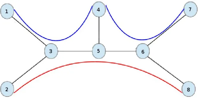
Figure 1. An example of a network with three connections and seven links.
Let us considern TCP connections operating in an Internet Protocol (IP) network ofL links defined by a routing matrixA, whose element alk is equal to one if connection k goes through
link l, or zero otherwise. Without loss of generality, we assume that each link is occupied by some connection, and each connection is routed through some link. Denote byxk(t) the sending
rate of connectionkat time t. We also denote byP(k) the set of links constituting to the path of connectionk. An example of such a network is sketched in Figure 1, where we specify a link with the two nodes it connects. For example, (1,3) denotes the link between nodes 1 and 3. Let us label all the links in the following way.
label 1 2 3 4 5 6 7
link (1,3) (3,5) (4,5) (5,6) (6,7) (2,3) (6,8)
the connections 1, 2, 3 are routed over the paths P(1) ={1,2,3},P(2) ={3,4,5} and P(3) = {2,4,6,7}, respectively, so that the routing matrix is given by
A=
1 0 0 1 0 1 1 1 0 0 1 1 0 1 0 0 0 1 0 0 1
.
In this section, the column vector notationx(t) := (x1(t), . . . , xn(t))T is in use, and the terms
of connection and source are used interchangeably.
We point out that our network model is quite general at least in the following sense. The data sources are allowed to use different TCP versions, or if they use the same TCP, the TCP parameters (round-trip time, the increase-decrease factors) can be different. More precisely, we suppose that the sending rate of connectionk evolves according to the following equation
d
dtxk(t) =akx
γk(t), a
k∈(0,∞), γk∈[0,1], (12)
follows
xk(Ti,k) =bkxk(Ti,k−)< xk(Ti,k−), bk∈(0,1). (13)
Here and below,ak,bk and γk are constants, which would cover at least two important versions
of the TCP end-to-end congestion control; if γk = 0 we retrieve the AIMD congestion control
mechanism (see Avrachenkov et al. (2010)), and ifγk= 1 we retrieve the Multiplicative Increase
Multiplicative Decrease (MIMD) congestion control mechanism (see Kelly (2003), Zhang et al. (2010)). Also note that (12) and (13) correspond to a hybrid model description that represents well the saw-tooth behavior of many TCP variants, see Hespanha et al. (2001), Avrachenkov et al. (2010), Zhang et al. (2010).
When Ti+2,k > Ti+1,k =Ti,k > Ti−1,k, multiple (indeed, two in this case) congestion
notifica-tions are being sent out simultaneously atTi+1,k =Ti,k. We only allow finitely many congestion
notifications to be sent out at any time moment. For now we writeTi := (Ti,1, . . . , Ti,n) for the ith time moments of the impulsive control for each of the n connections, and assume that the decision of reducing the sending rate of connectionkis independent upon the other connections. Since there is no gradual control, we tentatively call the sequence ofT1, T2, . . . a policy for the congestion control problem, which will be formalized below.
We will consider two performance measures of the system; namely the time averageα-fairness function
lim inf
T→∞
1 1−α
n
X
k=1 1 T
Z T
0
x1k−α(t)dt,
and the discountedα-fairness function
lim inf
T→∞
1 1−α
n
X
k=1
Z T
0
e−ρTx1k−α(t)dt,
to be maximized over the consecutive moments of sending congestion notifications Ti, i =
1,2, . . .. In the meanwhile, due to the limited capacities of the links, the expression lim infT→∞ T1 R0T Ax(t)dt (resp., lim infT→∞R0T e−ρtAx(t)dt) under the average (resp.,
dis-counted) criterion should not be too big. Therefore, after introducing the weight coefficients λ1, . . . , λL≥0,we consider the following objective functions to be maximized:
Q=
n
X
k=1
(
lim inf
T→∞
1 T
Z T
0
x1k−α(t) 1−α dt
)
−
L
X
l=1 λl
X
k:l∈P(k) lim inf
T→∞
1 T
Z T
0
xk(t)dt (14)
in the average case, and
Qρ= n
X
k=1
(
lim inf
T→∞ Z T
0
e−ρtx 1−α k (t)
1−α dt
)
−
L
X
l=1 λl
X
k:l∈P(k) lim inf
T→∞ Z T
0
e−ρtxk(t)dt (15)
in the discounted case, where we recall that P(k) indicates the set of links corresponding to connectionk.
Below by using the verification theorems established earlier, we obtain the optimal policies for the problems
Q→ max
T1,T2,...
and
Qρ→ max T1,T2,...
, (17)
respectively.
3.1 Solving the average optimal impulsive control problem
We consider in this subsection the average problem (16). Concentrated on policies satisfying
lim inf
T→∞
1 1−α
n
X
k=1 1 T
Z T
0
x1k−α(t)dt= lim
T→∞
1 1−α
n
X
k=1 1 T
Z T
0
x1k−α(t)dt <∞
and lim infT→∞ T1 R0T xk(t)dt < ∞ for each k = 1, . . . , n, for problem (16) it is sufficient to
consider the case ofn= 1.Indeed, one can legitimately rewrite the function (14) as
Q=
n
X
k=1 lim inf
T→∞
1 T
Z T
0
x1k−α(t) 1−α −λ
kx k(t)
!
dt,
where λk := P
l∈P(k)λl, which allows us to decouple different sources. Thus, we will focus on
the case ofn= 1, and solve the following optimal control problem
˜
J(x0) = lim inf T→∞
1 T
Z T
0
x1−α(t)
1−α −λx(t)
dt→ max
T1,T2,...
, (18)
wherex(t) is subject to (12), (13) and the impulsive controlsT1, T2, . . . with the initial condition x(0) =x0.Here and below the indexk= 1 is omitted for convenience.
In the remaining part of this subsection, using the verification theorem (Theorem 2.3), we rigorously obtain the optimal policy and value to problem (18) in closed-forms.
Remark 3 : When more than one but finitely many congestion notifications are sent out si-multaneously, in line with the treatment in the previous section, we will understand the resulting multiple reductions on the sending rate as a consequence of a single “big” impulsive control.
Let us start with formulating the congestion control problem (18) in the framework given in the previous section, which also applies to the next subsection. Indeed, one can take the following system parameters;X = (0,∞), j(x, v) =bvx,C(x, v) = 0 withv ∈V ={1,2, . . .}, f(x, u) =axγ,andc(x, u) = x11−−αα −λx withu∈U,which is a singleton, i.e., there is no gradual control, so that in what follows, we omitu∈U everywhere.
For the future reference and to improve the readability, we write down the Bellman equation (9) for problem (18) as follows;
max
x1−α
1−α −λx
−g+∂h ∂x(x)ax
γ, sup m=1,2,...
{h(bmx)−h(x)}
= 0. (19)
As will be seen in the next theorem, for each fixed x, the supremum inside the parenthesis of (19) is attained at a finite value of m.
Theorem 3.1 : Suppose λ > 0, γ ∈ [0,1], α > 0, α 6= 1, 2−α −γ 6= 0, a ∈ (0,∞),
π∗= (L∗, vL∗) with L∗= [x,∞), andvL∗(x) =k if x∈[bkx−1,bxk)⊆ L
∗ for k= 1,2, . . . ,where
¯ x=
(2−γ)(1−b2−α−γ) (2−α−γ)(1−b2−γ)λ
α1
>0. (20)
When γ <1, the value function is given by
J(x0, π∗) =g:=xλ
α 1−α
(1−γ)(1−b2−γ)
(2−γ)(1−b1−γ); (21)
and whenγ = 1,
J(x0, π∗) =g:=xλ
α 1−α
b−1
ln (b). (22)
(Clearly, the constructed policy π∗ is admissible.)
The proof of this theorem can be found in the appendix.
3.2 Solving the discounted optimal impulsive control problem
The discounted problem turns out more difficult to deal with, for which we consider that the sending rate increases additively, i.e., dxk(t)
dt = ak > 0, and decreases multiplicatively, i.e., j(xk, v) =bkxk with bk∈(0,1) when a congestion notification is sent, see (12) and (13). Thus,
the prevailingly used version of TCP New Reno in today’s Internet is covered as a special case. Furthermore, we assumeα∈(1,2).
Similarly to the average case, we concentrate on policies under which lim infT→∞
RT
0 e
−ρtx
k(t)dt = limT→∞ RT
0 e
−ρtx
k(t)dt < ∞, and upon rewriting the
objec-tive function in problem (17) as Qρ = Pnk=1lim infT→∞ RT
0 e
−ρtx1k−α(t)
1−α −λkxk(t)
dt, where
λk = P
l∈P(k)λl, it becomes clear that there is no loss of generality to focus on the case of n= 1;
˜
Jρ(x0) = lim inf T→∞
Z T
0 e−ρt
x1−α(t)
1−α −λx(t)
dt→ max
T1,T2,...
, (23)
As in the average case, one can put this impulsive control problem in the framework of the previous section; see Remark3 and the paragraph above it, so that Theorem 2.5 is applicable. Now the Bellman equation (11) has the form
max
x1−α
1−α−λx−ρW(x) +a dW
dx , supi≥1
[W(bix)−W(x)]
= 0. (24)
The linear differential equation
x1−α
1−α −λx−ρW˜(x) +a dW˜
dx = 0 (25)
can be integrated:
˜
W(x) =eρa(x−1)
λ ρ +
λa ρ2 +
1
ρ(α−1)+ ˜w1
− x
1−α ρ(α−1)−
λ ρx−
aλ ρ2 −
eρax
ρ
Z x
1
Here ˜w1 = ˜W(1) is a fixed parameter.
Suppose for a moment that no impulses are allowed, so that x(t) = x0+at. We omit the π index because here is a single control policy. We have a family of functions ˜W(x) depending on the initial value ˜w1, but only one of them coincides with the objective function
lim inf
T→∞ Z T
0
e−ρt(x(t)) 1−α
1−α −λx(t)
dt=W∗(x0).
In this situation, for the function ˜W, all the parts of Condition 2.4 are obviously satisfied (D=∅, T1 =∞,L∗=∅) except for (iv).
Since W∗ <0, the case lim supT→∞e−ρTW∗(x(T))>0 is excluded and we need to find such
an initial valuew∗1 that lim
T→∞e
−ρTW˜(x(T)) = 0, where x(T) =x
0+aT, x0 >0. (27) Equation (27) is equivalent to the following:
lim
T→∞e ρ ax0
e−ρa
λ ρ +
λa ρ2 +
1
ρ(α−1)+ ˜w1
−1 ρ
Z x0+aT
1
e−ρauu−αdu
= 0.
Therefore,
w∗1 = e
ρ a
ρ
ρ
a
α−1
Γ
1−α,ρ a
− 1
ρ(α−1)−
λ(ρ+a)
ρ2 , (28)
and W∗(x0) is given by (26) with ˜w1 = w1∗. Here Γ(y, z) =
R∞
z e
−uuy−1du is the incomplete gamma function (Gradshteyn and Ryzhik 2007, 3.381-3).
For the discounted impulsive control problem (17), the solution is given in the following state-ment.
Theorem 3.2 : The following statements take place. (a) Equation
H(x) :=eρx(1a−b) −1
(1−b)λa
ρ −(1−b)e
ρx a
Z x
bx
e−ρuau−αdu (29)
−eρx(1a−b) −b
x1−α(1−b1−α)
α−1 +λx(1−b)
= 0
has a single positive solution x¯. (b) Let
w1 = e
ρ a
ρ
Z x¯
1
e−ρuau−αdu−λ(ρ+a)
ρ2 − 1
ρ(α−1) (30)
−
"
¯
x1−α(1−b1−α) ρ(α−1) +
(1−b)λx¯
ρ +
eρbax¯
ρ
Z x¯
bx¯
e−ρauu−αdu #,
eρbx¯a−ρ −e ρ¯x−ρ
a
and, for 0< x <x¯, put W(x) = ˜W(x), where W˜ is given by formula (26) under w1˜ =w1. For the intervals x,¯ x¯b, x¯b,bx¯2
(c) The functionW(x0) = supπJρ(x0, π) =Jρ(x0, π∗) is the Bellman function, where the
(feed-back) optimal policy π∗ is given by
L∗ = [¯x,∞), vf,L∗(x) =i if x∈h x¯ bi−1,
¯ x bi
.
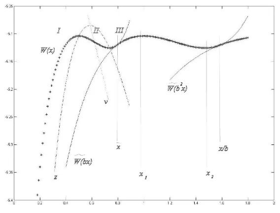
See the appendix for the proof. The shape of the Bellman functionW is plotted in Figure A1.
Remark 4 : Let us calculate the limit of ¯x whenρ approaches zero. One can easily show that, for any x >0,
lim
ρ→0H(x) = 0 and ρlim→0 H(x)
ρ =
x2(1−b) a
λ(b2−1)
2 +
x−α(1−b2−α) 2−α
.
Let
¯ x0=
2(1−b2−α) λ(1−b2)(2−α)
1/α
, (31)
i.e.
lim
ρ→0 H(x)
ρ
>0, ifx <x¯0, <0, ifx >x¯0, = 0, ifx= ¯x0.
The function Hρ(x) is continuous with respect to ρ. Therefore, for any small enough ε >0,
∃δ >0 : ∀ρ∈(0, δ) H(¯x0−ε)
ρ >0 and
H(¯x0+ε) ρ <0
meaning that ¯xρ, the solution to (29) at ρ ∈ (0, δ), satisfies ¯xρ ∈ (¯x0−ε,x0¯ +ε). This means
limρ→0+x¯ρ = ¯x0. Note that (31) is the optimal threshold if we consider the long-run average reward with the same reward ratec.
Remark 5 : The two theorems established in this section define our proposed threshold-based AQM scheme, which asserts that if the sending rate is smaller than ¯x, then do not send any congestion notification, while if the sending rate is greater or equal to ¯x,then send (multiple, if needed) congestion notifications until the sending rate is reduced to some level belowx with x given by (20) under the average criterion and by Theorem 3.2(a) under the discounted criterion.
4 Conclusion
Appendix A:
A.1 Proof of Theorem 3.1
Proof of Theorem 3.1.Supposeγ <1. By Theorem 2.3, it suffices to show that Condition 2.2 is satisfied by the policyπ∗= (L∗, vL∗), the constantg given by (21) and the function
h(x) =
h0(x), ifx∈(0,x¯),
hk(x) =h0(bkx),ifx∈[¯x/bk−1,x/b¯ k),
(A1)
where
h0(x) = 1 a
− x
2−α−γ
(1−α)(2−α−γ) +λ x2−γ 2−γ +g
x1−γ 1−γ
,
and ¯xis given by (20). Standard analysis shows that the functionh is bounded from below, and so Condition 2.2 is satisfied. Since part (i) of Condition 2.2 is trivially verified, we only verify its parts (ii,iii) as follows.
Consider firstly x ∈ (0, x) = X \ L∗. Then, we obtain from direct calculations that
x1−α
1−α −λx
− g + ∂h∂x(x)axγ =
x1−α
1−α −λx
− g + ∂h0(x)
∂x axγ = 0. Let us show that
supm=1,2,...{h(bmx)−h(x)} = supm=1,2,...{h0(bmx)−h0(x)} ≤ 0 for x ∈ (0, x) as follows. De-fine ∆1(x) :=h0(bx)−h0(x) for each x ∈ (0, x). Then one can show that ∆1(x) <0 for each b∈(0,1).Indeed, direct calculations give
∆1(x) = x1−γ
a
−(b
2−α−γ−1)x1−α
(1−α)(2−α−γ) +λ
(b2−γ−1)x 2−γ +g
(b1−γ−1) 1−γ
,
so that for the strict negativity of ∆1(x), it is equivalent to showing it for the following expression ˜
∆1(x) :=−
(b2−α−γ−1)x1−α
(1−α)(2−α−γ) +λ
(b2−γ−1)x
2−γ +g
(b1−γ−1)
1−γ ,
whose first order and second order derivatives (with respect tox) are given by
˜
∆01(x) =−(b
2−α−γ−1)x−α
2−α−γ +λ
(b2−γ−1) 2−γ
and
˜
∆001(x) = α(b
2−α−γ−1)x−α−1 2−α−γ .
Under the conditions of the parameters, ˜∆001(x) < 0 for each x ∈(0, x), and thus the function ˜
∆1(x) is concave on (0, x) achieving its unique maximum at the stationary point given by x = x = n(2(2−−αγ−)(1γ)(1−b−2−b2α−−γγ))λ
oα1
> 0. Note that ˜∆1(x) = 0 and limx↓0∆˜1(x) ≤ 0. It follows from the above observations and the standard analysis of derivatives that ˜∆1(x) <0 and thus ∆1(x)<0 for each x∈(0, x).Since ∂x∂b ≤0 for each b∈(0,1) as can be easily verified, one can replaceb withbm (m= 2,3, . . .) in the above argument to obtain thath
0(bmx)−h0(x)<0 for eachx∈(0, x), and thus
sup
m=1,2,...
forx∈(0, x),as desired. Hence, it follows that Condition 2.2(ii,iii) is satisfied on (0, x). Next, we show by induction that Condition 2.2(ii,iii) is satisfied on [bkx−1,
x
bk),k= 1,2, . . . .Let
us consider the case ofk= 1, i.e., the interval [¯x,x¯b). By the definition of the function h(x), we have
sup
m=1,2,...
{h(bmx)−h(x)}= 0 (A3)
forx∈[¯x,x/b¯ ). Indeed, by the definition ofh(x), we have
h(bx)−h(x) = 0 (A4)
for x ∈ [¯x,x/b¯ ), whereas for each m = 2,3, . . . and x ∈ [¯x,x¯b), it holds that h(bmx)−h(x) = h0(bmx)−h0(bx) ≤ 0, which follows from that bx ∈ (0, x), bmx = bm−1(bx) ∈ (0, x) for each x∈[¯x,x¯b),and (A2). Furthermore, one can show that
∆2(x) := x1−α
1−α −λx−g+ ∂h(x)
∂x ax
γ ≤0 (A5)
for eachx∈[¯x,x/b¯ ),which follows from the following observations. Sinceh(x) =h1(x) =h0(bx), we see ∆2(x) =−(b
2−α−γ−1)x1−α
1−α +λ(b2
−γ−1)x+g(b1−γ−1) for eachx∈[¯x,¯x
b),and in particular,
∆2(x) = 0, (A6)
as can be easily verified. The derivative of the function ∆2(x) with respect to x is given by ∆02(x) = −(b2−α−γ−1)x−α +λ(b2−γ−1). If 2−γ−α < 0, then ∆02(x) < 0, which together with (A6) shows ∆2(x)≤0 on [¯x,x¯b).If 2−γ−α > 0, then ∆200(x) =α(b2−α−γ−1)x−α−1 <0 and thus, the function ∆2(x) is concave with the maximum attained at the stationary point x=
1−b2−α−γ
(1−b2−γ)λ 1
α
.Since
1−b2−α−γ
(1−b2−γ)λ 1
α
≤x, (A6) implies ∆2(x)≤0 on [¯x,x¯b),as desired. By the way, for the later reference, the above observations actually show that
G(x) :=−(b
2−α−γ−1)x1−α
1−α +λ(b
2−γ−1)x+g(b1−γ−1)≤0 (A7)
for all x≥x. Thus, combining (A3), (A4), and (A5) shows that Condition 2.2(ii,iii) is satisfied on [¯x,x¯b).
Assume that for each x ∈[bkx−1,
x
bk) and each k = 1,2, . . . , M, relations (A3) and (A5) hold,
together with
h(bkx)−h(x) = 0 (the corresponding version of (A4)). (A8) Now we consider the case of k = M + 1, i.e., when x ∈ [bxM,
x
bM+1). For each x ∈ [
x bM,
x bM+1),
when m = 1,2, . . . , M, it holds that bmx ∈ [bMx−m,bM+1x−m), and thus h(bmx) − h(x) =
h0(bM+1x) − h0(bM+1(x)) = 0; when m = M + 1, M + 2, . . ., bmx ∈ (0, x) = L∗, and thus h(bmx) − h(x) = h0(bmx) − h0(bM+1x) = 0 if m = M + 1, and h(bmx) − h(x) = h0(bm−(M+1)(bM+1x))−h0(bM+1x) ≤ 0 if m > M + 1, by (A2). Thus, we see (A3) holds forx∈[bxM,
x
bM+1). Note that in the above we have also incidentally verified the validity of (A8)
for the case ofk=M+ 1.
eachk= 1,2, . . . ,sinceh(x) =hk(x) =h0(bkx) for each x∈[bkx−1,bxk), we have
∆2(x) :=−
(bk(2−α−γ)−1)x1−α
(1−α) +λx(b
k(2−γ)−1) +g(bk(1−γ)−1).
For the convenience of the future reference, let us introduce the notation
˜
∆k(x) :=−
(bk(2−α−γ)−1)x1−α 1−α +λ(b
k(2−γ)−1)x+g(bk(1−γ)−1)
= bk(1−γ)(−b
k(1−α)x1−α
1−α +λb
kx+g)−(−x1−α
1−α +λx+g)
for each x >0.Therefore, for x∈[bkx−2,
x
bk−1), we have
∆2(x) = ˜∆k−1(x) =b(k−1)(1−γ)(−
b(k−1)(1−α)x1−α 1−α +λb
k−1x+g)−(−x1−α
1−α +λx+g).
Let us define
F(x) :=−x 1−α
1−α +λx+g
for each x >0.We then have from the direct calculations that
˜ ∆k−1(
¯ x bk−2) =b
(k−1)(1−γ)F(bx¯)−F( x¯
bk−2) (A9)
for each k= 1,2, . . . .Focusing on F(bkx¯−2),we have
b1−γF( x¯
bk−2) =− ¯ x1−α 1−α
b1−γ
b(k−2)(1−α) +λx¯ b1−γ bk−2 +gb
1−γ
=−x¯ 1−α
1−α
b2−α−γ
b(k−1)(1−α) +λx¯ b2−γ bk−1 +gb
1−γ
=−( ¯ x b(k−1))1
−α
1−α b
2−α−γ+λ( x¯ bk−1)b
2−γ+gb1−γ.
Recall that in the above, we have proved that G(x) ≤ 0 for x ≥ x¯, see (A7). Thus, we have G(bk¯x−1)≤0,i.e.,−
b2−α−γ( x¯ bk−1)
1−α
1−α +λb2
−γ( x¯
bk−1)+gb1
−γ ≤ −(bk¯x−1) 1−α
1−α +λ( ¯ x
bk−1)+g.Consequently,
b1−γF( x¯
bk−2)≤ − (bkx¯−1)1
−α
1−α +λ( ¯ x
bk−1) +g=F( ¯ x bk−1).
Now we verify (A5) for the particular case ofk=M+ 1. By the inductive supposition, (A5) holds for x∈[bMx−1,
x
bM), we thus have ∆2(
¯ x
bM−1)≤0, and
0≥∆˜M(
¯ x
bM−1) =b
M(1−γ)F(bx¯)−F( x¯
bM−1)≥b
(M)(1−γ)F(bx¯)− 1 b1−γF(
¯ x bM).
Therefore, we obtain thatb(M+1)(1−γ)F(bx¯)−F(bx¯M)≤0,and by (A9),
∆2( ¯ x
Furthermore, the derivative of the function ˜∆M+1(x) with respect to x is given by ˜∆0M+1(x) = −(b(M+1)(2−α−γ)−1)x−α+λ(b(M+1)(2−γ)−1). If 2−γ −α < 0, then ˜∆0M+1(x) < 0. Thus, by (A10), we obtain that ∆2(x) = ˜∆M+1(x) ≤ 0 for x ∈ [bxM,bMx+1). If 2−γ −α > 0, then
˜
∆00M+1(x) = α(b(M+1)(2−α−γ) −1)x−α−1 < 0, and in turn, the function ˜∆M+1(x) is concave with the maximum attained at the stationary pointx=
1−b(M+1)(2−α−γ)
(1−b(M+1)(2−γ))λ α1
.Moreover, we have PM
m=0b
m(2−α−γ)
PM
m=0bm(2−γ)
≤ bM α1 ,which follows from the fact that for eachm= 0,1, . . . , M, m(2−α−γ) +
M α≥m(2−γ),so that bm(2−α−γ)bM α≤bm(2−γ). From this we see
(1−b2−α−γ)PM
m=0bm(2−α−γ) (1−b2−γ)PM
m=0bm(2−γ)
≤ 1
bM α
1−b2−α−γ 1−b2−γ
⇒ 1−b
(M+1)(2−α−γ) (1−b(M+1)(2−γ))λ ≤
1 bM α
(2−γ)(1−b2−α−γ)
(2−α−γ)(1−b2−γ)λ
⇔ 1−b
(M+1)(2−α−γ) (1−b(M+1)(2−γ))λ
!(1 α)
≤ x¯ bM.
Finally, it follows from the last line of the previous inequalities, the concavity of the function ˜
∆M+1 and (A10) that ∆2(x)≤0 forx∈[bxM,
x
bM+1), which verifies (A5), and thus completes the
proof.
For the case ofγ = 1, we consider the functionh in the form of (A1) with ¯x being still given by (20), andh0 being defined by
h0(x) = 1 a
− x
1−α
(1−α)2 +λx+glnx
.
Condition 2.2(i, ii, iii) can be verified similarly to the case ofγ <1.We now focus on the verifica-tion of Condiverifica-tion 2.2(iv). Ifα >1, theng <0,and standard analysis shows thath0 is bounded from below, so that Condition 2.2(iv) is verified. Consider the case of α < 1. Then g > 0, and any policy π satisfying lim supt→∞ h(x
π(t))
t <0 cannot be optimal. Indeed, it follows from
lim supt→∞ h(x π(t))
t <0 that for each >0,there exists someT >0 such thath(x
π(t))≤ −tfor
allt > T.Therefore, limt→∞h(xπ(t)) =−∞.Since− x
1−α
(1−α)2+λxis bounded on [0, x],necessarily
limt→∞xπ(t) = 0.But then lim inft→∞1t Rt
0
(xπ(s))1−α
1−α −λx
π(s)ds = 0< g (c.f. (18)).
There-fore, it suffices to consider policiesπ which verify Condition 2.2(iv), i.e., lim supt→∞ h(x π(t))
t ≥0.
Now the statement follows from Remark2.
A.2 Proof of Theorem 3.2
Some comments and remarks are in position before we give the proof of this theorem. In fact, they help the reader follow the proof. For b= 0.5,ρ = 1,α = 1.3, λ= 2, a= 0.2 the graph of the functionW is presented in Figure A1. Here ¯x= 0.7901 andw1 =−4.9301. The dashed line represents the graph of the function
z(x) =−1 ρ
x1−α α−1 +λx
When ˜W(x) = z(x), we have ddxW˜ = 0; if ˜W(x) > z(x) (resp., ˜W(x) < z(x)), the function ˜W increases (resp., decreases). The dotted line represents the graph of the function
v(x) = a(x
−α−λ) ρ2 −
1 ρ
x1−α α−1 +λx
.
If ˜W(x) =v(x),then from (25) we have
a2d 2W˜ dx2 =a
2
"
aρdW˜
dx +λa−ax
−α
#
=a2
ρ2W˜(x) +ρλx+ρx 1−α
α−1 +λa−ax
−α
= 0,
[image:17.595.146.430.288.504.2]that is, x is the point of inflection of the function ˜W. This reasoning applies to any solution of equation (25).
Figure A1. Graph of the Bellman functionW(x) (bright line with the star point markers).
In the graph, for 0 < x < x¯, the Bellman function W(x) = ˜W(x) has three parts, denoted below as I, II and III, where it increases, strictly decreases, and again increases. Correspondingly, the function ˜W(bx) also has three parts I, II and III, where it increases, strictly decreases and increases again, andW(x) = ˜W(bx) for ¯x≤x < x¯b. The point ¯x is such that
˜
W(¯x) = ˜W(bx¯) and dW˜(x) dx
¯ x
= dW˜(bx) dx
¯ x
. (A12)
As is shown in the proof of Theorem 3.2 below, these two equations are satisfied if and only if ¯
xsolves equation (29).
branch above function v because the two increasing functions ˜W(x) and ˜W(bx) could not have common points.
The increasing part I of function ˜W(x) cannot intersect with ˜W(bx).
The strictly decreasing part II of the function ˜W(x) cannot intersect with the parts II and III of the function ˜W(bx). Possible common points with the part I of ˜W(bx) are of no interest
because here dW˜dx(x) <0 and dW˜dx(bx) ≥0.
The increasing part III of function ˜W(x) can intersect with the parts I and II of function ˜
W(bx), but again the latter case is of no interest because here dW˜dx(x) ≥0 and dW˜dx(bx) <0. Thus, the only possibility to satisfy (A12) is the case when the increasing part III of ˜W(x) touches the increasing part I of function ˜W(bx). The inflection linev(x) is located between the increasing and decreasing branches of the functionz(x), so that the part III of ˜W(x) is convex and the part I of ˜W(bx) is concave, meaning that no more than one point ¯x can satisfy the equations (A12).
Using formula (26), the equations (A12) can be rewritten as follows:
0 = ˜W(x)−W˜(bx) =eρxa −e bρx
a
e−ρa
λ ρ +
λa ρ2 +
1
ρ(α−1)+ ˜w1
−1 ρ
Z x 1
e−ρua u−αdu
−x
1−α(1−b1−α)
ρ(α−1) −(1−b) λx
ρ + ebρxa
ρ
Z bx x
e−ρuau
−αdu;
(A13)
0 = dW˜(x) dx −
dW˜(bx) dx =
ρ ae
ρx a −bρ
ae
bρx a e−
ρ a λ ρ + λa ρ2 +
1
ρ(α−1)+ ˜w1
−1 ρ
Z x
1
e−ρua u−αdu
−(1−b)λ ρ +
bebρxa
a
Z bx
x
e−ρuau−αdu.
After we multiply these equations by factors 1−be(b−1)ρxa
and aρ1−e(b−1)ρxa
correspond-ingly and subtract the equations, the variable ˜w1 is cancelled and we obtain equation
0 =
1−be(b−1)ρxa
"
b1−αx1−α ρ(α−1) +
ebρxa
ρ
Z bx
x
e−aρuu−αdu−
x1−α
ρ(α−1)−(1−b) λx ρ # −a ρ
1−e(b−a1)ρx
"
bebρxa
a
Z bx
x
e−ρuau−αdu−(1−b)λ
ρ
#
,
which is equivalent toH(x) = 0.
Equation (30) follows directly from the first one of equations (A13): if we know the value ofx (equal to ¯x), we can compute the value of ˜w1 =w1.
To prove the solvability of the equation (29) we compute the following limits:
lim
x→∞H(x)≤ −xlim→∞e ρx(1−b)
a ·λx(1−b) =−∞;
lim
x→0H(x) = limx→0(b−1)
x1−α(1−b1−α) α−1 +
Z x
bx
e−ρuau−αdu
,
and the positive expression in the square brackets does not exceed
x1−α(1−b1−α) α−1 +
Z x
bx
1−ρu a + 1 2 ρu a 2
u−αdu= x
+
u1−α 1−α −
ρu2−α a(2−α) +
ρ2u3−α 2a2(3−α)
x
bx
=
ρ2u3−α 2a2(3−α) −
ρu2−α a(2−α)
x
bx
→0 as x→0,
so that limx→0H(x) = 0. Finally,
dH dx =−
ρ(1−b) a e
ρx(1−b) a
x1−α(1−b1−α)
α−1 +λx(1−b)
+
b−eρx(1a−b)
λ(1−b)−x−α(1−b1−α)+λ(1−b)2eρx(1a−b)
−ρ
a(1−b)e
ρx a
Z x
bx
e−ρuau−αdu−(1−b)e ρx
a h
e−ρxax−α−be− ρbx
a (bx)−α i
=−ρ(1−b)(1−b 1−α) a(α−1) x
1−α−
b−1−ρx(1−b) a
(1−b1−α)x−α−λ(1−b)
+λ(1−b)2− ρ a(1−b)
x1−α(1−b1−α) 1−α
−(1−b)
1 +ρx a
x−α
1−ρx a
−b
1−ρbx a
(bx)−α
+(x),
where limx→0(x) = 0; so
lim
x→0 dH
dx = limx→0
ρ(1−b)(1−b2−α)
a x
1−α = +∞
meaning that the continuous function H(x) increases from the limit zero for small values of x and becomes negative for big values ofx.
Therefore, equation (29) has a single positive solution ¯x, and part (a) of the statement has been proved.
(b) Item (i) of Condition 2.4 is obviously satisfied (D=∅). For Item (ii), we consider the following three cases.
(α) Let 0 < x ≤ x¯. The differential equation (25) holds for function W on the interval 0< x <x¯. For these values of x,
W(bix)< W(x),∀ i≥1. (A14) Indeed, to prove this, note that the functionW(bx) = ˜W(bx) is increasing (c.f. Figure A1), so that W(bx) > W(b2x) > . . . . As explained in the proof of part (a), Part III of the function W(x) is convex and the function ˜W(bx) touching smoothlyW(x) at the point ¯x, is concave, so that W(bx) = ˜W(bx) < W(x) here. The same inequality holds for smaller values of x where W(x) decreases (part II) andW(bx) = ˜W(bx) increases. Part I of the functionW(x) is obviously bigger than W(bx), too. Thus the Bellman equation (24) is satisfied on the interval 0< x < x¯ and also on the interval (0,x¯].
(β) Consider x ∈ (¯x,x/b¯ ] and denote x1 and x2 the points of the analytical maximum and minimum of the functionW(x) = ˜W(bx). (See Fig.A1.)
Forx∈(¯x, x1) the functionW(x) is concave; hence
a dW dx x
< a dW dx ¯ x
=a dW˜ dx ¯ x
=ρW˜(¯x)− x¯ 1−α
1−α +λx¯=ρ[ ˜W(¯x)−z(¯x)].
have
adW dx
x
< ρ[W(x)−z(x)] =ρW(x)−
x1−α 1−α −λx
,
and the Bellman equation (24) is satisfied because hereW(x) = ˜W(bx) =W(bx) andW(bi+1x)< W(bx) for all i≥1 by (A14).
Forx∈[x1, x2] we haveW(x)> z(x) andadWdx ≤0: remember,W(x) = ˜W(bx) and the latter function is of type II forx∈[x1, x2]. Therefore, again
adW dx −ρ
W(x)−1 ρ
x1−α 1−α −λx
<0
and the Bellman equation (24) is satisfied. Forx∈(x2,x/b¯ ], we have
adW dx =b
dW˜ dx
bx < dW˜
dx
bx
because the function ˜W increases here andb∈(0,1). Next,
ρ[W(x)−z(x)] =ρ[ ˜W(bx)−z(x)]> ρ[ ˜W(bx)−z(bx)]
because the functionz(x) decreases. Therefore,
adW
dx −ρ[W(x)−z(x)]< dW˜
dx
bx
−ρ[ ˜W(bx)−z(bx)] = 0
sincebx≤x¯, and, for these values, equation (25) holds. We see that the Bellman equation (24) is satisfied.
(γ) Finally, let us consider the remaining interval (x¯b,∞).Suppose
adW
dx −ρ[W(x)−z(x)]<0 forx∈
x¯
bi−1, ¯ x bi
i
,
for some naturali≥1. Then, for x∈ bx¯i,
¯ x bi+1
, we have
adW
dx −ρ[W(x)−z(x)] =ba dW
dx
bx
−ρ[W(bx)−z(x)].
If dWdx
bx<0 then the last expression is negative. Otherwise, ba dW
dx
bx
≤a dW dx
bx
andz(x)< z(bx),
so that
adW
dx −ρ[W(x)−z(x)]< a dW
dx
bx
−ρ[W(bx)−z(bx)]<0
Thus, the Bellman equation (24) is satisfied for allx >0.
To finish the proof of part (b) of this statement, it remains to note that Item (iii) of Condition 2.4 is also obviously satisfied:
L∗ = [¯x,∞); vf,L∗(x) =vi ifx∈
h x¯
bi−1, ¯ x bi
.
(c) Note that item (iv) of Condition 2.4 is not satisfied. Indeed, there is an admissible control policy such that, on any time interval (T−1, T],xπ(·) is so close to zero thate−ρTW(xπ(T))<−1. (Remember that limx→0W(x) =−∞.)
Let us fix an arbitrary x0 >0 and modify the reward rate:
ˆ c(x) =
c(x), ifx≥min{x0, bx¯}:= ˆx; c(ˆx), ifx <x.ˆ
Note that ˆc ≥ c. The function ˜W(x) given by (26) will change only for x < xˆ ≤ x0 and remains increasing in its part I, meaning that this modified function ˆW satisfies all items (i)– (iii) of Condition 2.4: the proof is identical to the one presented above. But now Condition 2.4 (iv) is also satisfied because the function ˆW is bounded. Therefore, according to Theorem 2.5, supπJˆρ(x0, π) = ˆW(x0) = ˆJρ(x0, π∗), where ˆJρ corresponds to the reward rate ˆc. But
sup
π
Jρ(x0, π)≤sup π
ˆ
Jρ(x0, π) = ˆW(x0) =W(x0),
and for the feedback policyπ∗, which is independent ofx0, we have W(x0) = ˆW(x0) = ˆJρ(x0, π∗) =Jρ(x0, π∗).
The last equality holds because, under the feedback policyπ∗, starting from x0, the trajectory xπ∗(t) satisfiesxπ∗(t)≥xˆfor all t≥0, and in this region ˆc=c.
Acknowledgement
This work is partially funded by INRIA Alcatel-Lucent Joint Lab, ADR “Semantic Networking”.
References
Altman, E., Avrachenkov, K., and Prabhu, B. (2005), “Fairness in MIMD Congestion Control Algorithms,” Telecommunication Systems, 30, 387–415.
Avrachenkov, K., Ayesta, U., and Piunovskiy, A. (2010), “Convergence of trajectories and opti-mal buffer sizing for AIMD congestion control,” Performance Evaluation, 67, 501–527. Bardi, M., and Capuzzo-Dolcetta, I., Optimal Control and Viscosity Solutions of
Hamilton-Jacobi-Bellman Equations, Boston: Birkhauser (1997).
Bensoussan, A., and Lions, J., Impulse Control and Quasivariational Inequalities, Montrouge: µ, Gauthier-Villars (1984).
Christensen, S. (2014), “On the solution of general impulse control problems using superharmonic functions,” Stochastic Processes and Their Applications, 124, 709–729.
Davis, M.,Markov Models and Optimization, London: Chapman and Hall (1993).
Gradshteyn, I., and Ryzhik, I., Table of Integrals, Series, and Products, New York: Academic Press (2007).
Hespanha, J.P., Bohacek, S., Obraczka, K., and Lee, J. (2001), “Hybrid Modeling of TCP Con-gestion Control,” Hybrid Systems: Computation and Control, LNCS v. 2034, pp. 291–304. Hordijk, A., and van der Duyn Schouten, F. (1983), “Average optimal policies in Markov decision
drift processes with applications to a queueing and a replacement model,” Advances in Applied Probability, 15, 274–303.
Hou, S., and Wong, K. (2011), “Optimal impulsive control problem with application to human immunodeficiency virus treatment,” Journal of Optimization Theory and Applications, 151, 385–401.
Kelly, F.P., Maulloo, A.K., and Tan, D. (1998), “Rate control for communication networks: shadow prices, proportional fairness and stability,” Journal of the Operational Research Society, 49, 237–252.
Kelly, T. (2003), “Scalable TCP: Improving performance in high-speed wide area networks,”
Computer Communication Review, 33(2), 83–91.
Korn, R. (1999), “Some applications of impulse control in mathematical finance,”Mathematical Methods of Operations Research, 50, 493–518.
Kunniyur, S., and Srikant, R. (2003), “End-to-end congestion control schemes: utility functions, random losses and ECN marks,” IEEE/ACM Transactions on Networking, 11, 689–702. Li, Y.T., Leith, D., and Shorten, R. (2007), “Experimental Evaluation of TCP Protocols for
High-Speed Networks,”IEEE/ACM Transactions on Networking, 15, 1109–1122.
Low, S.H., and Lapsley, D.E. (1999), “Optimization flow control I: basic algorithm and conver-gence,” IEEE/ACM Transactions on Networking, 7, 861–874.
Miller, A., and Miller, B. (2011), “Control of connected Markov chains. Application to congestion avoidance in the Internet,” In Proceedings of IEEE CDC-ECC 2011, pp. 7242–7248. Miller, B., and Rubinovich, E.,Impulsive Control in Continuous and Discrete-Continuous
Sys-tems, New York: Springer (2003).
Mo, J., and Walrand, J. (2000), “Fair end-to-end window-based congestion control,”IEEE/ACM Transactions on Networking, 8, 556–567.
M¨oller, N., Barakat, C., Avrachenkov, K., and Altman, E. (2007), “Inter-protocol fairness be-tween TCP New Reno and TCP Westwood,” in3rd EuroNGI Conference on Next Genera-tion Internet Networks, pp. 127–134.
Motta, M., and Rampazzo, F. (1996), “Dynamic programming for nonlinear systems driven by ordinary and impulsive controls,”SIAM Journal on Control and Optimization, 34, 199–225. Noirie, L., Dotaro, E., Carofiglio, G., Dupas, A., Pecci, P., Popa, D., and Post, G. (2009), “Semantic networking: Flow-based, traffic-aware, and self-managed networking,” Bell Labs Technical Journal, 14, 23–38.
Palczewski, J., and Stettner, L. (2007), “Impulsive control of portfolios,” Applied Mathematics and Optmization, 56, 67–103.
Piunovskiy, A. (2004), “Multicriteria impulsive control of jump Markov processes,”Mathematical Methods of Operations Research, 60, 125–144.
Taringoo, F., and Caines, P. (2013), “On the optimal control of impulsive hybrid systems on Riemannian manifolds,”SIAM Journal on Control and Optimization, 51, 3127–3153. Xiao, Y., Cheng, D., and Qin, H. (2006), “Optimal impulsive control in periodic ecosystem,”
Systems and Control Letters, 55, 558–565.
Yushkevich, A. (1989), “Verification theorems for Markov decision processes with controllable de-terministic drift, gradual and impulse controls,”Theory of Probability and Its Applications, 34, 474–496.