virginia mazzini
virginia mazzini
S P E C I F I C - I O N E F F E C T S I N
N O N - A Q U E O U S S O L U T I O N S
December 2017
A thesis submitted for the degree of Doctor of Philosophy of The Australian National University
University © December2017.
e-mail: virginia.mazzini@anu.edu.au
This document was typeset using LATEX and Lorenzo Pantieri’sArsClassicapackage, a reworking of the ClassicThesis style designed by André Miede, inspired to the masterpieceThe Elements of Typographic Styleby Robert Bringhurst.
Graphics were typeset using the tikz package, to achieve continuity of the typo-graphic style in text and typo-graphics. Calculations were performed, and plots made,
inR(R Core Team, 2017), using mainly the packagesplyrand ggplot2; the
pack-agetikzDevicewas employed to translate theRgraphics into LATEXtikz-pgf com-mands.
This thesis is an account of my own original research work, undertaken between May2013and December2017at the Department of Applied Math-ematics in the Research School of Physics and Engineering at the Australian National University (Canberra, Australia).
Parts of the contents presented have been produced in collaboration with colleagues, and published or submitted for publication in peer-reviewed journals. These are listed in the section ‘List of Publications’ and are clearly marked in the body of the document.
None of this material has been submitted in whole or part to any other insti-tution for the award of a degree or diploma. To the best of my knowledge, this thesis contains no work previously published by another person, except where due reference is made in the text.
This research is supported by an Australian Government Research Training Program (rtp) Scholarship.
This manuscript contains approximately40000words.
I acknowledge and celebrate the First Australians on whose traditional lands I have been living during the production of this thesis, and I pay my respect to the elders of the Ngunnawal people past and present.
Canberra, December2017
A C K N O W L E D G E M E N T S
I am grateful to all that have supported me, professionally and/or personally, during this demanding journey.
I thank my supervisor Prof. Vince Craig for providing positive incentives, creative and honest scientific discussions, genuine advice, and for striving to adapt his supervision methods to the different needs of his students. I am particularly grateful for the opportunities of development and networking Prof. Craig has enabled me to attend, and for his commitment to promoting an inclusive and diverse research environment.
My advisor Prof. Pierandrea Lo Nostro has introduced me to the topic of specific-ion effects, and has been a participating mentor since my Masters’ studies. I am thankful for the scientific guidance, the lifting conversations in moments of discouragement, and for the light-hearted humour.
Dr. Drew Parsons, also in the role of advisor, has willingly given assistance in some more abstract aspects of my research. In addition, I am appreciative of the fruitful discussions that I have shared with Dr. Andrea Salis during his time as a visiting fellow in the Department of Applied Mathematics; and of the caring advisory support and frank opinions provided by Prof. Barry Ninham.
I also have received invaluable technical support for the completion of my work. I am indebted to Mr. Tim Sawkins and Mr. Ron Cruikshank at the Department of Applied Mathematics for general technical support; to Mr. David Anderson, Mr. Dennis Gibson and Mr. Luke Materne of the Re-search School of Physics and Engineering Electronics Unit at the anu— es-pecially for assembling the ‘button-bot’; to Ms. Bozena Belzowski, Mrs. Avis Paterson and Mr. Vance Lawrence at theanuResearch School of Chemistry for providing Blue Dextran; to Dr. Fouad Karouta from the Department of Electronics Materials Engineering for granting access to experimental equip-ment.
On a personal note, I am blessed with the friendship and affection of many. I thank my parents Katia and Gino, for being devoted to us daughters, and for educating us in the values of laicism, freedom, progress and solidarity. My sister Elisa, endless love and priceless wit. I look forward to reading your thesis. Manuela and Massimo, for welcoming me as your own daughter and hosting me and chauffeuring me around Florence and Prato when I visited.
ison, E-Jen, Rick, Matt, Ben and all the other fellow students and researchers in the Applied Mathematics Department.
A B ST R A C T
Electrolyte solutions play a central role in life and technological processes because of their complexity. This complexity is yet to be described by a pre-dictive theory of the specific effects that different ions induce in solution. The vast majority of investigations of specific-ion effects have been conducted in aqueous solutions. These studies have revealed that amongst the complexity, the effectiveness of the ions often follow trends that are apparent across a number of very different experiments, revealing an underlying order, (e.g. the Hofmeister series). It is often assumed that water itself is intricately involved in these trends.
Here I investigate specific-ion effects in non-aqueous solvents rather than water. By extending the investigation to a number of non-aqueous solvents, the role of the solvent in specific-ion effect trends can be elucidated and a better understanding of the general phenomenon gained.
Firstly, a more definite terminology is developed for describing the speci-fic-ion effects trends in order to address the current confusion in the liter-ature and provide a basis for the following investigations. An extensive investigation of the scarce literature demonstrates that water is by no means a special solvent with regards to ion-specificity, and that within the com-plexity there is universality. An investigation of electrostriction under the conditions of infinite dilution shows that the same fundamental specific ion trends are observed across all solvents, demonstrating that ion-specificity arises from the ions themselves. In this regard the influence of solvents, sur-faces and real concentrations of electrolytes can be seen as perturbations to this fundamental series. Further work shows that for systems that are per-turbed, the trends in non-aqueous protic solvents can be expected to follow the same trend in water; and in aprotic solvents the cations are more likely to adhere to the trend in water than the anions.
My experimental work focuses on specific-anion effects of seven Hofmeis-ter sodium salts in the solvents: waHofmeis-ter, methanol, formamide, dimethyl sulfoxide and propylene carbonate. Two very different experiments were performed; the elution of electrolytes from a size-exclusion chromatography column and an investigation of the electrolyte moderated swelling of a cat-ionic brush (pmetac) using a Quartz Crystal Microbalance (qcm). The trends observed are consistent across these experiments. A forward or re-verse Hofmeister series is observed in practically all salt-solvent combina-tions, and the reversal is attributed to the polarisability of the solvent.
If you think education is expensive, try ignorance.
C O N T E N T S
list of figures xvii list of tables xxi
list of acronyms & abbreviations xxiii list of symbols xxv
list of publications xxxi
1 introduction 1
1.1 The importance of specific-ion effects 1 1.2 A brief historical account of sie 2 1.3 Theories of ion-specificity 3
1.4 An experimentalist’s point of view 5 1.5 Motivations for this work 6
1.6 Non-aqueous electrolytes 7 1.7 Outline of the thesis 7
2 literature review 9 2.1 Introduction 9
2.2 Manifestations of sie 10 2.3 Terminology 11
2.4 Characteristics of non-aqueous solvents 15 2.5 Methodology 17
2.6 Methanol 19 2.7 Formamide 21
2.8 N-methylformamide 22 2.9 N,N-dimethylformamide 23 2.10 Dimethyl sulfoxide 24 2.11 Additional solvents 25 2.12 Other investigations 28 2.13 An overall view 30 2.14 Summary 32
3 electrostriction 35 3.1 Motivation 35
3.2 Partial molar volumes and electrostriction 36 3.3 Methods 38
3.4 Results and discussion 41 3.5 Conclusions 54
4 volcano plots 57 4.1 Introduction 57
4.2 Energies related to the solvation process 58
4.3 The origin of volcano plots 59
4.4 The law of matching water affinities 61 4.5 Brief review of recent volcano plot studies 62 4.6 Results and discussion 68
4.7 Interpretation of volcano plots in solvents 73 4.8 Volcano plots in the ‘real world’ 81
4.9 Conclusions 84
5 experimental procedures 87 5.1 Experimental materials 87
5.2 Preparation of the salt solutions 90
5.3 The influence of trace quantities of water 93 5.4 Material incompatibilities with the solvents 97
6 chromatography of salts 99 6.1 Rationale 99
6.2 Size-exclusion chromatography in water 99 6.3 Description of the technique 101
6.4 Experiment details 103
6.5 Results and detailed discussion 113 6.6 Summary 120
7 anion-specific polymer conformation 123 7.1 Introduction 123
7.2 Qcm for investigating polymer conformation 124 7.3 Experiment details 126
7.4 results and discussion 131 7.5 Summary 134
8 an overall view 135
8.1 A global depiction of sie in non-aqueous solvents 135 8.2 The global experiment picture of anion trends 139
9 conclusions 143 9.1 Further work 145
a electrostriction data 147 a.1 Tabulation of the volumes 147
Bibliography for the current appendix 151 a.2 Standard molar volumes of electrolytes 152 a.3 Electrostrictive volume of electrolytes 154 a.4 Normalised electrostrictive volumes 156
b volcano plots 159
b.1 Aqueous ionic radii versus ab initio radii 159 b.2 Lines highlighting cation trends 160
b.3 Lines highlighting anion trends 164 b.4 Solubilities of electrolytes in solvents 169
contents xv
c.2 Plots 180
Bibliography for the current appendix 186
d solubility data collection 191
Bibliography for the current appendix 200
e custom conductivity cell 203
f effect of water impurities on sec and qcm experiments 205 f.1 Size-exclusion chromatography 205
f.2 Polymer conformation byqcm 208 f.3 Conclusions 208
g a summary of unsuccessful approaches 209 g.1 Standard molar volume measurements 209 g.2 Turbidimetry 212
g.3 Nmr T2 relaxation times of salt solutions 212
g.4 Swelling of commercial hydrogels 212
L I ST O F F I G U R E S
Figure1 Hofmeister and lyotropic series of ions 13 Figure2 concentration dependence of electrostriction 38 Figure3 electrostrictive volumes scheme 39
Figure4 intrinsic volumes of electrolytes 41
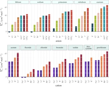
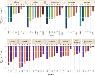
Figure5 standard molar volumes of electrolytes in water 42 Figure6 electrostrictive volumes of electrolytes in water 48 Figure7 normalised electrostriction in water 49
Figure8 Born-Haber cycle of the solvation-related enthalpies 59 Figure9 volcano plots, free energies, cation trends 71
Figure10 radii volcano plots, enthalpies, cation trends 74 Figure11 radii volcano plots, free energies, cation trends 75 Figure12 protic volc. p. polyatomic anions, enthalp., cat. trends 77 Figure13 aprotic volc. p. poly. anions, enthalp., cat. trends 78 Figure14 radii protic volc. p., poly. anions, enthalp., cat. trends 79 Figure15 radii poly. anions aprot. volc. p., enthalp., cat. trends 80 Figure16 volcano plots, activity coefficients, cation trends 83 Figure17 molecular models of the experiments chemicals 89 Figure18 scheme of the chromatography experiment setup 104 Figure19 custom-made conductivity detector calibration curves 106 Figure20 chromatogram of sodium electrolytes in water 114 Figure21 chromatogram of sodium electrolytes inmeoh 116 Figure22 chromatogram of sodium electrolytes in fa 117 Figure23 chromatogram of sodium electrolytes in dmso 119 Figure24 chromatogram of sodium electrolytes in pc 120 Figure25 summary ofsec retention factors 121
Figure26 pmetac skeletal structural formula 123
Figure27 qcm shifts, dependence on salt concentration 129 Figure28 qcmshifts, brush-coated sensor versus bare sensor 130 Figure29 qcm,pmetacbrush net response to concentration 130 Figure30 qcm, solvent-dependent effect of NaClO4onpmetac 131
Figure31 summary ofqcm shifts in all solvents 133 Figure32 qcm,∆D3 versus−∆F3 plot 134
Figure33 standard molar volumes of electrolytes inmeoh 152 Figure34 standard molar volumes of electrolytes inetoh 152 Figure35 standard molar volumes of electrolytes in fa 152 Figure36 standard molar volumes of electrolytes innmf 152 Figure37 standard molar volumes of electrolytes in eg 152 Figure38 standard molar volumes of electrolytes in pc 153 Figure39 standard molar volumes of electrolytes in ec 153 Figure40 standard molar volumes of electrolytes indmso 153 Figure41 standard molar volumes of electrolytes in ace 153 Figure42 standard molar volumes of electrolytes inmecn 153 Figure43 standard molar volumes of electrolytes indmf 153
Figure44 electrostrictive volumes of electrolytes inmeoh 154 Figure45 electrostrictive volumes of electrolytes in etoh 154 Figure46 electrostrictive volumes of electrolytes in fa 154 Figure47 electrostrictive volumes of electrolytes in nmf 154 Figure48 electrostrictive volumes of electrolytes in eg 154 Figure49 electrostrictive volumes of electrolytes in pc 155 Figure50 electrostrictive volumes of electrolytes in ec 155 Figure51 electrostrictive volumes of electrolytes indmso 155 Figure52 electrostrictive volumes of electrolytes in ace 155 Figure53 electrostrictive volumes of electrolytes inmecn 155 Figure54 electrostrictive volumes of electrolytes in dmf 155 Figure55 normalised electrostriction inmeoh 156
Figure56 normalised electrostriction inetoh 156 Figure57 normalised electrostriction infa 156 Figure58 normalised electrostriction innmf 156 Figure59 normalised electrostriction ineg 156 Figure60 normalised electrostriction inpc 157 Figure61 normalised electrostriction inec 157 Figure62 normalised electrostriction indmso 157 Figure63 normalised electrostriction inace 157 Figure64 normalised electrostriction inmecn 157 Figure65 normalised electrostriction indmf 157 Figure66 hydrated versusab-initioradii of ions 159
Figure67 volcano plots, protic, enthalpies, cation trends 160 Figure68 volcano plots, aprotic , enthalpies, cation trends 160
Figure69 exploded volcano plots, protic, enthalpies, cation trends 161 Figure70 exploded volcano plots, aprotic , enthalpies, cat. trends 161 Figure71 volcano plots, osmotic coefficients, cation trends 162 Figure72 poly. anions volcano plots, osmotic coeff., cation trends 163 Figure73 poly. anions volcano plots, activity coeff., cation trends 163 Figure74 volcano plots, protic, enthalpies, anion trends 164
Figure75 volcano plots, aprotic , enthalpies, anion trends 164 Figure76 volcano plots, protic, free energies, anion trends 165 Figure77 volcano plots, aprotic , free energies, anion trends 165 Figure78 radii volcano plots, protic, enthalpies, anion trends 166 Figure79 radii volcano plots, aprotic , enthalpies, anion trends 166 Figure80 radii volcano plots, protic, free energies, anion trends 167 Figure81 radii volcano plots, aprotic , free energies, anion trends 167 Figure82 volcano plots, osmotic coeff., anion trends 168
Figure83 volcano plots, activity coeff., anion trends 168 Figure84 electrolyte solubility in protic solvents 169 Figure85 electrolyte solubility in aprotic solvents 170 Figure86 osmotic coeff. of alkali metal halides 180 Figure87 activity coeff. of alkali metal halides 181
list of figures xix
L I ST O F TA B L E S
Table1 Hofmeister original experiment series 3
Table2 physical properties of the solvents investigated 16 Table3 specific-ion effects series in water 18
Table4 sie series inmeoh 19
Table5 additional sieseries in meoh 20 Table6 sie series infa 21
Table7 sie series innmf 23 Table8 sie series indmf 24 Table9 sie series indmso 25 Table10 sie series inetoh 26 Table11 sie series inpc andec 27
Table12 additional sieseries in pcand ec 28
Table13 summary ofsie series in different solvents 31 Table14 anionsie trends in standard molar volumes 43 Table15 cationsie trends in standard molar volumes 44 Table16 anionsie trends in electrostrictive volumes 46 Table17 cationsie trends in electrostrictive volumes 47 Table18 anionsietrends in the normalised electrostriction 51 Table19 cationsietrends in normalised electrostriction 52 Table20 summary of volcano plots reported in the literature 65 Table21 specifications of the electrolytes used in experiments 88 Table22 oven drying protocol for the electrolytes 88
Table23 technical specifications of the solvents investigated 90 Table24 solubility of electrolytes in non-aqueous solvents 92 Table25 summary of the electrolytes investigated per solvent 93 Table26 contaminant water to ion ratio 94
Table27 size of investigated ions and solvent molecules 100 Table28 sec column size in different solvents 110
Table29 summary of the anion-specific trends from experiment 139 Table30 ab initiostatic ionic polarisabilities 141
Table31 intrinsic, standard, electrostrictive and normalised volumes 147 Table32 Pitzer model fitting coeffs. in non-aqueous solvents 173
Table33 Pitzer-Archer model coeffs. in non-aqueous solvents 177 Table34 Polynomial fitting coefficients non-aqueous solvents 177 Table35 Pitzer coefficients for electrolytes in water 178
Table36 literature salt solubility in non-aqueous solvents 191
A C R O N Y M S & A B B R E V I AT I O N S
1pentoh 1-pentanol (pentan-1-ol). 198 2buoh 2-butanol (butan-2-ol).192
2proh 2-propanol (propan-2-ol). 16,173,177,199
ace acetone (propan-2-one). 16, 25, 30–32, 38, 42– 47,50–52,150,153,155,157,173,191
acs American Chemical Society.88,90
buoh butanol (butan-1-ol). 70,191,192
dlvo Derjaguin, Landau, Verwey, Overbeek.4 dma N,N-dimethylacetamide. 16,173,192 dmc dimethyl carbonate. 173
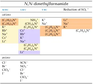
dme dimethoxyethane (1,2-dimethoxyethane). 173 dmf N,N-dimethylformamide. 16,23,24,26,30–32,
38, 43, 44, 46, 47, 51, 52, 95, 150, 151,153, 155, 157,173,192,193
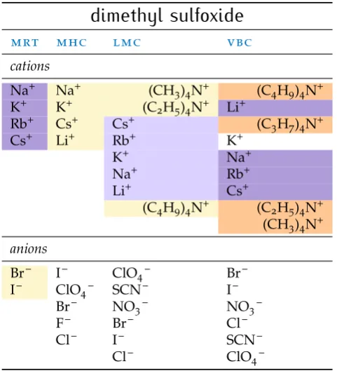
dmso dimethyl sulfoxide. 7,16,24–26, 29–32,38, 43, 44, 46, 47, 51, 52, 83, 90, 91, 93–95,97,99, 100, 103, 106, 109, 110, 112, 113, 116, 119–121, 127, 128, 132, 134, 139–142, 144, 149, 150, 153, 155, 157,162,163,168,173,174,177,193,205,207
ec ethylene carbonate (1,3-dioxolan-2-one). 16, 25–28, 30–32, 38, 42–44, 46, 47, 51, 52, 66, 68, 83,149,153,155,157,162,168,174,177,193 eg ethylene glycol (ethane-1,2-diol). 16,25,28,30,
31, 38, 42–44, 46, 47, 51, 52, 70, 148, 149, 152, 154,156,193
etoh ethanol. 7, 16, 25–27, 29–31, 38, 43–47, 51, 52, 148,152,154,156,174,177,193,194
fa formamide. 7, 16,21,22,24, 28, 30–32,38,43– 47, 51, 52, 70, 90, 93, 94, 97, 99, 100, 103, 106, 109, 110, 112, 113, 116–119, 121, 122, 127, 128, 132, 134, 139–142, 144, 148, 152, 154, 156, 194, 212
fep fluorinated ethylene propylene. 98,105
ft-ir Fourier-transform infrared spectroscopy. 28, 102
i-buoh iso-butanol (2-methylpropan-1-ol).192
i-pentoh iso-pentanol (3-methylbutan-1-ol). 198
kf Karl Fischer. 90,91,94–97,205
lmc limiting molar ionic conductivity. 15, 18, 19, 21–27,30–32,48,53,118,122
lmwa law of matching water affinities. 8, 29, 37, 57, 60–64, 66–68, 81, 82, 84, 89, 101, 118, 124, 143, 172
md molecular dynamics simulations. 4,64
mecn acetonitrile. 7, 16, 25, 29–31, 38, 43, 44,46, 47, 51, 52, 85, 95, 141, 150, 153, 155, 157, 174,194, 195
meno2 nitromethane. 25,30–32,141,195
meoh methanol. 7,16,19–21,29–32,38,43–47,51,52, 67, 70, 82, 83, 85, 90, 93–97, 99, 100, 103, 105– 107, 109–113, 115–117, 119–122, 127, 130–134, 139–141, 144, 147, 148, 152, 154, 156, 162, 168, 174, 175, 177, 195–197, 205, 206, 208, 209, 211, 212
mhc constant pressure standard partial molar heat capacity of the ion. 18–21,23–27,31,32,48 mrt nmrmolecular reorientation time. 18–25,31 msa- methanesulfonate. 28
nma N-methylacetamide. 83, 141, 162, 163, 168, 175–177,197
nmf N-methylformamide. 16, 22–26,30–32, 38, 43– 47, 51, 52, 83, 84, 150, 152, 154, 156, 162, 168, 176,197
nmr nuclear magnetic resonance. 17,20,29,61,102, 111,125,145,212
list of acronyms & abbreviations xxv
peek polyether ether ketone. 105
pmetac
poly(2-methacryloyloxyethyl-trimethyl-ammonium chloride. 123, 124, 127, 129–134, 140
proh 1-propanol (propan-1-ol).16,25,30,31,72,198, 199
ptfe polytetrafluoroethylene.98,105,106,108,128
qcm quartz crystal microbalance. 8, 91, 95, 97, 98, 122, 124, 126–129, 131, 132, 134, 139, 140, 205, 208
qcm-d quartz crystal microbalance with dissipation monitoring. 125–127
rdd relative limiting static dielectric decrement. 18, 19,21–23,31,32
sec size-exclusion chromatography. 8, 95, 98, 99, 101, 102, 114, 115, 120–122, 134, 138–140, 144, 203,205,206
sie specific-ion effects. 1–12,14,15,17,19–28, 30– 33, 35, 37, 43–47, 51–55, 57, 62, 64, 84, 85, 87, 89, 90, 93–95, 99, 113, 122, 131, 132, 134–145, 205
sulf sulfolane (tetrahydrothiophene 1,1-dioxide). 163,176,177
t-buoh tert-butanol (2-methylpropan-2-ol). 141,192
vbc viscosityB-coefficients (see Bη). 15, 18, 19, 21–
L I ST O F SY M B O L S
α static polarisability. 16,141 αp isobaric expansivity. 211
AN Gutmann-Mayer acceptor number. 16, 17, 19, 70
Bη B-coefficients from the empirical Jones-Dole
viscosity equation. 37, 48, 53, 61, 65–67, 83, 85
ci amount-of-substance concentration of solute i,
unitsmol dm−3. 90,210–212 CN coordination number. 65
Dn QCM dissipation factor of the overtone n
2Γn/fn. 125,126
∆Dn shift of — . 126,128,129,132,134
DN Gutmann donor number. 15,16,19,70
η viscosity.16
0 electric constant or vacuum permittivity,
8.854×10⁻¹²F m−1. 171
R relative permittivity. 16,38,60,171
e elementary charge,1.602 176 634×10−19C.60, 171
fn QCM resonance frequency of the overtone n.
125,126
∆fn shift of the — . 126,128–131,133,134,208
∆Fn normalised — — . 129–134,208
γ activity coefficient. 82, 83, 163, 168, 171–176, 181,183,185
Γn QCM half-height half-bandwidth of the
over-tone n. 125
∆abs. hydr.G−◦ absolute standard molar Gibbs free energy of
hydration (solvation in water). 65
∆abs. soln.G molar Gibbs free energy of solvation. 58
∆abs. soln.G−◦ absolute standard — . 58,70,71,78,165
∆fG−◦ standard molar Gibbs free energy of formation. 58
∆hydr.G−◦ standard molar Gibbs free energy of dissolu-tion in water. 65
∆soln.G−◦ standard molar Gibbs free energy of
dissolu-tion.58,69,71,75,78,80,165,167
∆abs. hydr.H−◦ absolute standard molar enthalpy of hydration
(solvation in water). 65
∆abs. soln.H molar enthalpy of solvation. 58
∆abs. soln.H−◦ absolute standard — . 58,59,70,77,160,164
∆fH−◦ standard molar enthalpy of formation. 58, 59,
69
∆hydr.H molar enthalpy of dissolution in water. 60
∆hydr.H−◦ standard molar — . 65,69
∆soln.H−◦ standard molar enthalpy of dissolution. 58,59,
69,74,77,79,160,164,166
k Boltzmann constant,1.381×10−23J K−1. 171 Ka association constant.65
Kav size exclusion chromatography available
reten-tion factor.102,111,115 Kd dissociation constant. 65
Ksec size exclusion chromatography retention
factor.101,102,111,113,120,121
kT isothermal compressibility.16,38
µ dipole moment.16
Mi molar mass of species i ing mol−1. 3, 16, 40,
100,111,115,209–211
mi molality of solute i, units mol kg−1. 90, 171–
185,210
νi stoichiometric coefficient of species i. 3
Na Avogadro constant6.022×1023mol−1. 171
N% electrostrictive volume normalised by the in-trinsic volume. 49–53,147–151,156,157
ni number of moles of species i in mol. 36, 94, 209,210
π 3.1415926536. 100,125,171
φ osmotic coefficient. 65, 66, 162, 163, 168, 171, 172,180,182,184
P pressure. 36,209
list of symbols xxix
ρi density of species i ing cm−3. 16,40,191–200,
209–212
ri radius of species i. 60,65,74,75,79,80,83,100,
159,162,163,166–170
S solubility. 65,82,92,169,170,191–200
∆abs. soln.S molar entropy of solvation. 58
∆fS−◦ standard molar entropy of formation. 58
T absolute temperature inK. 36,58,171,174–179, 209
t temperature in◦C. 16,88,92,191–200
V volume.36,100,209
Vcryst partial molar volume of a species in its
crystal-line form. 40
Vi partial molar volume of the species i in
solu-tion. 36,209
V−i◦ standard — . 36,38,39, 41–44, 49, 53,147–153, 209–211
φ
Vi apparent — . 209–212
Vi intr intrinsic molar volume of the species i. 36,38,
40,41,49,147–151
Vi el electrostrictive partial molar volume caused by the speciesi. 36
V−i el◦ standard — . 36,38,46–49,147–151,154,155 Vi internal pore volume of a stationary phase.
101,102,110–114,116,117,119,120 Vr elution volume of an analyte. 101,102
Vt total geometric volume of a stationary phase.
102,110,111,114,116,117,119,120
V0 void volume of a chromatography column.
101,102,110–114,116,117,119,120
Wt.% percentage by weight. 92,94,97, 111,191–200, 205
L I ST O F P U B L I C AT I O N S
Part of the work presented in this thesis has been published in the following papers:
Mazzini, V. and V. S. J. Craig
2016 ‘Specific-ion effects in non-aqueous systems’,Curr. Opin. Colloid In-terface Sci.23, pp.82–93,doi:10.1016/j.cocis.2016.06.009.
2017 ‘What is the fundamental ion-specific series for anions and cations? Ion specificity in standard partial molar volumes of electrolytes and electrostriction in water and non-aqueous solvents’,Chem. Sci.8(10 2017), pp.7052–7065,doi:10.1039/C7SC02691A.
2018 ‘Volcano plots emerge from a sea of non-aqueous solvents: The law of matching water affinities extends to all solvents’, Submitted. Mazzini, V., G. Liu and V. S. J. Craig
2018 ‘Probing the Hofmeister series beyond water: Specific-ion effects in non-aqueous solvents’, J. Chem. Phys. 148, 22, p. 222805, doi: 10 . 1063/1.5017278.
1
I N T R O D U C T I O N
The phrase ‘specific-ion effects (sie)’ encompasses all those cases where a property of an electrolyte solution, or the behaviour of a substance dissolved therein, depends on the particular cations and anions present beyond their electrostatic charge.
1.1 the importance of specific-ion effects
Between the years2000 and2017, Web of Science™ indexes more than 1700 publications investigating sie, that span across (bio)chemistry, (bio)physics, materials science, biotechnology, pharmacology, engineering, medicine, wa-ter resources and plant science. This inwa-terdisciplinary inwa-terest in siestems from the fact that electrolyte solutions are omnipresent: pure, neat water containing no dissolved salts is extremely rare in nature.
Salts are what enables the specificity and complexity of interactions in life processes. Everyone is aware of the essential role water has for life, but it is often overlooked that this water must be salty to be of any use: drink-ing demineralised water for long periods of time has deleterious effects on health due to osmotic shock and disruption of the body homeostasis mechan-isms (Kozisek,2005). The details of ‘life’ is one of the most pressing research topics. Untangling its mechanisms and one day explaining its mystery is a major ambition of scientific progress. This cannot be achieved without ac-knowledging the importance of salts for life: ions interact with proteins and affect their solvated structure (Baldwin, 1996; Y. Zhang and Cremer, 2006); the activity of enzymes is salt-dependent (Bilaniˇcová et al., 2008). Striking examples are provided by the fields of medicine and biology (Lo Nostro and Ninham,2012). The fine-tuned equilibrium that allows the human body to function largely relies on the specificity allowed by electrolytes. For in-stance, intravenous injections of NaCl and KCl solutions, that differ only by the cations they contain, both of charge+1, have dramatically distinct effects on a subject. The first one is known as saline solution, and can be injected to treat dehydration. The latter instead alters the resting potential of the cardiac muscle and can quickly induce death by cardiac arrest (Weidmann,
1956). Strict protocols are constantly discussed to avoid accidental adminis-tration of the latter to a patient (Reeve et al.,2005). An extensive account of
sie in biology can be found in:Kunz (2010),Lo Nostro and Ninham(2012) andNinham and Lo Nostro(2010).
Ions have a fundamental role in climate and natural equilibria as well. Sea-water is quite rich in a variety of ions, and as a consequence foams more than freshwater. One of the causes of the foaming of sea water (pollution and al-gae aside) is the presence of salts that inhibit bubble coalescence (Craig, Nin-ham et al.,1993a). Salts also reduce the solubility of gases in water (Millero, Huang et al.,2002a,b) and therefore affect aquatic life.
Important sie are also observed in a vast variety of other settings, such as the processing of colloids, where the stability (Lyklema, 2009) and rhe-ological behaviour of the system can be controlled (Franks, 2002; Franks et al., 1999). Also, the supramolecular self-assembly of surfactants is salt-dependent (Lo Nostro, Ninham, Ambrosi et al., 2003; Lo Nostro, Ninham, Milani et al., 2006). The above have consequences in applications such as mineral processing and wastewater treatment, and also in drug delivery and in food processing (cheesemaking for instance). In addition, polymer conformations show rich ion-specificity (Y. Zhang and Cremer, 2006), with consequences for instance in the development of responsive surface coat-ings (Azzaroni et al., 2005; G. Liu and G. Zhang, 2013; Willott et al., 2015; Y. Zhang, Furyk et al.,2005). Finally,sieare also relevant in corrosion kinet-ics (Trompette,2015).
1.2 a brief historical account of sie
The realisation that the electrostatic charge of an ion is not sufficient to de-scribe the properties of its solutions occurred early on, but the theoretical connection of solution behaviour to the fundamental properties of the elec-trolytes remains a work in progress.
Although Poiseuille already had worked on the electrolyte-dependent vis-cosity of salt solutions (Kunz, 2009), the work of Franz Hofmeister and col-laborators at the end of the19thcentury (Hofmeister,1888a,b) is considered
the starting point of the topic of sie in contemporary scientific literature. An English translation of this landmark work is available (Kunz, Henle et al.,2004).
1.3 theories of ion-specificity 3
Table 1:Values from Hofmeister’s original study on the precipitation of egg globulin (Hofmeister, 1888a; Kunz, Henle et al., 2004). Each cell shows the lowest concentration of the salt composed by the corresponding ions that is able to precipitate the protein. The concentration is expressed in Eq l−1, where the equivalent molar mass of each ion corresponds to its molar mass (Mi/g mol−1) divided by its stoichiometric coefficient (ν):
Eq=msalt/(Mcation/νcation+Manion/νanion), wheremsalt/gis the salt mass
per litre. The cell background shading highlights the groups individuated by Hofmeister based on the salt effectiveness in precipitating proteins. The darker the shade, the lower the salt precipitating power. The cells with the darkest shade and no value indicate salts for which no protein pre-cipitation could be achieved within their solubility interval. The grey cell indicates a salt with very poor solubility. Where the cell background is white, the salt has not been tested.
Li+ Na+ K+ NH4+ Mg2+ SO42– 1.57 1.60 2.03 2.65 HPO42– 1.65 1.61 2.51
CH3COO– 1.69 1.67 citrate3– 1.68 1.67 2.71 tartrate2– 1.56 1.51 2.72
HCO3– 2.53
CrO42– 2.62 2.64
Cl– 3.63 3.52
NO3– 5.42
ClO3– 5.53
et al.,2004). The explanation that he provided for this phenomenon was that salts withdraw water from the solubilised protein, causing it to precipitate. Different salts have different potency in ‘absorbing’ water. Hofmeister went on to test the generality of his hypothesis by salt-precipitating a range of very chemically distinct colloids: isinglass (collagen derived from the swim bladders of fish), colloidal ferric oxide and sodium oleate. Very similar re-sponses to the blood serum and egg globulin were found, consolidating the hypothesis and calling for further studies.
Research into siehas had surges in the following 150years, and exhaust-ive reviews of the literature and the evolution of scientific thought on sie are available (Cacace et al.,1997; Collins and Washabaugh, 1985;Jungwirth and Cremer, 2014; Kunz, Lo Nostro et al., 2004; Kunz and Neueder, 2009; Lo Nostro and Ninham,2012;Ninham and Lo Nostro,2010).
1.3 theories of ion-specificity
In fact, the classical theories that have been developed and employed dur-ing the19thand20thcentury, such as the Debye-Hückel theory of the activity
of strong electrolytes and theDerjaguin, Landau, Verwey, Overbeek (dlvo) theory for the stability of colloid suspensions, fail to predict the system be-haviour except for very dilute electrolyte solutions (close to ideality). As a consequence, the quantitative description of systems containing higher concentrations or more complex combinations of charged solutes, such as biological fluids, electrochemical solutions, the precipitation of colloids, the self-assembly of surfactants and the foaming of seawater have been inaccess-ible.
The restriction of the Debye-Hückel theory to dilute systems was clearly stated by its authors, but others nonetheless applied the theory as if it were a general one. Efforts focused on adding parameters and extensions in order to make this oversimplified model fit, rather than on the development of new approaches.
The classical theories are mainly based on electrostatic intuition. These models account for the non-ideality of electrolyte behaviour only at very dilute concentration, and the introduction of fitting parameters such as the ionic radii is needed to square with experimental values at higher concen-trations. That is, ion-specificity is not built into these models, and this is because they are not accounting for the Van der Waals forces, or they are not treating them adequately (Ninham and Yaminsky,1997). Van der Waals forces include all of the ‘electrodynamic’ forces: the collective and coordin-ated interactions of moving electrons (Parsegian,2006), and are further sub-divided into interactions between permanent dipoles (‘Keesom’ forces); in-teractions between a permanent dipole and the transient dipole induced in a nonpolar molecule by the permanent dipole itself (‘Debye’ forces); and interactions between transient dipoles of nonpolar but polarisable bodies (‘London’ dispersion forces) (Parsegian,2006). Dispersion forces depend on the particular ion: they are ion-specific and they are coupled to the electro-static forces, therefore a separate mathematical treatment of the two (that implies they are additive) is not satisfactory. In addition the potential needs to be calculated for many-body interactions, which are not pairwise additive: the body problem must be tackled. Although the inclusion of many-body quantum electrodynamics in the classical theories is widely agreed upon, this is not an easy task, and several groups are employing different approaches, mainly continuum treatments andmolecular dynamics simula-tions (md).
Concerted efforts to understand the fundamental origins of the Hofmeis-ter series and sie in general have emerged (Arslanargin et al., 2016; T. L. Beck,2011;Duignan, Baer and Mundy, 2016; Duignan, Baer, Schenter et al.,
1.4 an experimentalist’s point of view 5
2008; Ninham, Duignan et al., 2011; Ninham and Yaminsky, 1997; Pollard and T. L. Beck,2016,2017;Shi and T. Beck,2017).
This brief summary does not capture just how dynamic the theoretical work in the field currently is. In fact, there exists a plurality of positions on what details are most relevant in the theory, and even on where we are in our progress (that is, what remains to be understood). These are reflected in a number of publications and the following list is a brief selection: Boström et al. (2005), dos Santos et al. (2010), Gurau et al. (2004), Jungwirth and Cremer(2014),Kunz, Lo Nostro et al.(2004),Leontidis(2002,2016),Lo Nos-tro and Ninham (2012),Parsons, Boström, Lo Nostro et al. (2011), Pegram and Record(2008), Schwierz, Horinek and Netz(2010), Schwierz, Horinek, Sivan et al.(2016), Y. Zhang and Cremer (2006, 2010) and Y. Zhang, Furyk et al.(2005). Each approach offers benefits and time will reveal the realm in which these different treatments are best applied. Nevertheless, the outlook looks promising (Lo Nostro and Ninham,2016;Okur et al.,2017).
1.4 an experimentalist’s point of view
Developing an understanding of sie is a fundamental affair that has been actively investigated for a long time. It is compelling because of the wide-spread importance of electrolyte solutions across science and technology.
I would like to reflect here on my experience with sieas a university stu-dent. During my early studies, I acquired an understanding of electrolyte solutions that drew mainly on electrostatic intuitions, and on quantities diffi-cult to define such as hydration, hydrophobic forces or water structure. Only at an advanced stage I was exposed to the relevance of sie: despite being acquainted with the high level of specificity that chemistry implicates, the encounter was a wondrous one. Somehow I had assumed thatsiewere not that relevant and that our understanding of siewas crystalline. I therefore came to the conclusion that, across the uncountable experimental applica-tions and uses of electrolyte soluapplica-tions, a number of other scientists could be in my same situation. That is, that their deep knowledge of the specificities of the particular system at hand might not necessarily be accompanied by an appreciation of the generality of the phenomenon ofsie.
students at the start of their curricula, rather than to request a change in their forma mentis later. There are indeed cases where the effect of ions on a system are small with regards to the overall result, and in these cases the specific nature of the ions can be ignored, but this should be determined a posteriori.
1.5 motivations for this work
As the phenomenology of sie is very complex, and the theorisation dif-ficult, it is very hard to identify how the various interactions in solution balance, and what the overarching rules are. Everything seems to be equally relevant. This makes the work of theorists and experimentalists very diffi-cult. The present work aims at improving this condition, in the first place by attempting an identification of the dominant variables that affect sie in different experimental situations, and secondly by providing data that can offer a broader testing ground than those available so far in the literature.
The trigger for the research encompassed by this thesis was activated a few years ago by debate on the origin of sie. The main point of discussion was on the fundamental origin ofsie. Do they originate from the ions alone, from the interactions of the ions with the solvent, from the interaction of the ions with a surface, or a mix of all of the above?
A way to address the above questions is by investigating the solvent-dependency of sie, in order to ascertain the importance of the solvent. Whereas different types of ions and surfaces have been thoroughly analysed in relation to sie, the same detailed investigation has not yet been applied to solvents.
Some knowledge that the sie are evident in non-aqueous solvents was available prior to this work, but a comprehensive investigation into sie in non-aqueous solvents had not been conducted (Bilaniˇcová et al.,2008;Henry and Craig, 2008; Peruzzi, Ninham et al., 2012; Z. Yang, 2009). This work commenced seeking answers to the following questions: is water a special solvent in regards to manifestation of sie? If not, how do sie manifest in non-aqueous solvents — are the same trends as in water evident? Are there properties of the solvents or the ions directly or simply correlated to thesie trends? Are thesietrends experiment-dependent?
1.6 non-aqueous electrolytes 7
Ultimately, the expectation was that an improved knowledge ofsiein non-aqueous systems would advance our understanding of sie in aqueous sys-tems. As such, a theory that makes quantitative prediction ofsiein aqueous systems would also undergo the additional challenge of being tested against observations in non-aqueous solvents.
1.6 non-aqueous electrolytes
Although aqueous electrolytes have received the largest interest, non-aque-ous electrolyte solutions are relevant in a number of applications, particu-larly those encompassing electrochemical and electroanalytical aspects. This is because non-aqueous solvents offer a variety of advantages over aqueous solutions, that include different solvating properties, larger electrochemical windows and the prevention of hydration and hydrolysis (Zuman and Waw-zonek,1978). Drawbacks are the toxicity of many non-aqueous solvents, and in some cases the high volatility and flammability.
Examples include battery technology (Aurbach et al.,2004;Li et al.,2013; M. Winter and Brodd,2004); supercapacitors, whereacetonitrile (mecn)and propylene carbonate (4-methyl-1,3-dioxolan-2-one) (pc) are the solvents of choice (Béguin et al.,2014;M. Winter and Brodd,2004); electrodeposition of metals (Jorné and Tobias, 1975; Simka et al., 2009); semiconductors (Fulop and Taylor,1985;Lincot,2005;Nicholson,2005) including nanowires, as inR. Chen et al. (2003); conductive polymers (Ko et al., 1990) and fuel cells (M. Winter and Brodd,2004). Non-aqueous solvents are also employed in analyt-ical techniques such as non-aqueous capillary electrophoresis (Bjørnsdottir et al., 1998; Riekkola, 2002) and liquid chromatography (Jane et al., 1985) and are relevant in the rates of chemical reactions involving ionic transition states, such as Sn2 reactions (Parker, 1962). Non-aqueous solvents such as dimethyl sulfoxide (dmso) and formamide (fa) are also important in life sciences, the first in polymerase chain reaction (pcr) and as a cryoprotecting agent for the preservation of cells, tissues and organs; the latter as a dna denaturant. Methanol (meoh) and ethanol (etoh) are relevant in energy production. The systematic effect of different ions in the aforementioned ap-plications has been studied only in some cases, such as inLo Nostro, Mazzini et al.(2016).
1.7 outline of the thesis
These open with a review of the available literature in Chapter 2: in this chapter I identify the trends ofsiein a coherent way.
Chapter 3 is concerned with the fundamental trends of sie in different non-aqueous solvents by investigating the electrostrictive volume, a standard bulk property of solutions.
I consequently review the use of the ‘volcano plots’ and the law of match-ing water affinities (lmwa) concept in Chapter 4, and extend these to non-aqueous solvents, for standard thermodynamic properties such as the ener-gies of solution, but also for real-concentration ones: the activity coefficients and the solubility of electrolytes.
The exposition of my experimental work begins in Chapter5, with the gen-eral procedures and the materials employed, and the issues encountered; the results obtained in the size-exclusion chromatography (sec) of electrolytes experiments follow in Chapter 6; finally, the quartz crystal microbalance (qcm)investigations of the anion-specific conformation of polymer brushes are presented in Chapter7.
I discuss all the results obtained in this work collectively in Chapter 8 to give a general picture of this exploratory qualitative work on sie in non-aqueous solvents, and to outline its general implications.
In Chapter 9, I summarise the conclusions and delineate possible further work.
2
L I T E R AT U R E R E V I E W
This chapter is reproduced with revisions and changes from:
V. Mazzini and V. S. J. Craig (2016), ‘Specific-ion Effects in Non-aqueous Systems’, Curr. Opin. Colloid Interface Sci. 23, pp. 82–93, doi: 10 . 1016 / j . cocis.2016.06.009.
2.1 introduction
A reasonable starting point for this work is to review and analyse the avail-able knowledge onsiein non-aqueous solvents. This chapter therefore con-tains a review of the published literature on the matter, with the specific goal of looking fortrendsin thesiein non-aqueous systems. The analysis is performed with the following questions in mind:
1. Is a consistent trend in the strength ofsieseen in different experiments for the same non-aqueous solvent?
2. Do the trends in the strength of siein the non-aqueous solvents match those observed in water?
3. Are the trends observed in non-aqueous solvents consistent with the Hofmeister or lyotropic series?
4. Can the sieobserved be related to the properties of the solvent?
The present review is limited to works that explicitly investigate sie in non-aqueous solvents, as tracing publications that have only tangentially touched on the topic complicates the search due to the sprawled body of work on non-aqueous electrolytes.
In addition, only phenomena in neat solvents are covered. There is a con-siderable number of publications regarding electrolytes in mixed solvents, but this goes beyond the scope of this thesis, which addresses neat solvents only, as it is investigating the role of the solvent in sie. I regard mixed sol-vents as adding an additional level of complexity on the matter of sie in non-aqueous solvents, that is beyond the scope of this work.
The terminology that is going to be used is presented in Section2.3. The properties of the solvents investigated are listed in Table2.
A review summarising the general trends on the topic of sie in non-aqueous solvents has not previously been compiled, as pointed out recently
byKunz(2014), though Marcus has made a substantial contribution, in addi-tion to his large personal scientific producaddi-tion, in reviewing and tabulating the existing works regarding electrolytes in non-aqueous solvents (Jenkins and Marcus, 1995; Marcus, 2015; Marcus and Hefter, 2004; Marcus, Hefter and Pang, 1994). The gap is addressed here, with the aim to obtain insight into the general manifestation of siein non-aqueous solvents. This is made challenging by the scarcity and patchiness of the data on the behaviour of salts in non-aqueous solvents, which is partly due to the low solubility of electrolytes in many of them.
The majority of the data that are discussed in this chapter are contained in a recent book fromMarcus(2015). This is a carefully compiled work that includes critically tabulated data. It is a recent and updated collection of the state-of-the-art knowledge about aqueous and non-aqueous electrolyte solutions, and that makes it an invaluable reference for anyone interested in the topic.
2.2 manifestations of sie
The outcome of most measurements and experiments involving electrolyte solutions is dependent on the particular ions present (Kunz,2010;Lo Nostro and Ninham, 2012). The effect is most often observed as a modulation in the magnitude of a property (i.e. surface tension, conductivity, activity of enzymes) or as a difference in the concentration of electrolyte required to induce a particular change (such as in the precipitation of colloids and pro-teins). However and notably, in some cases, different ions of the same charge induce the opposite effect. Often the strength of the effect varies regularly across the anions and cations, even in systems that are dissimilar.
A large number of experimental works limit themselves to reporting the presence ofsiein a small set of electrolytes, without then attempting a more systematic study. Often, the recognition of sie is used as a self-standing explanation for the observed trend, as if the underlying mechanisms were fully understood. In a number of cases, the presence of a series is improp-erly claimed, as the electrolytes compared differ both in cations and anions, or only two salts have been considered. In order to produce work that is actually helpful in understanding sie, the electrolytes studied must share a common ion, otherwise it is not possible to separate the contribution of the anions and cations. Then, the minimum number of electrolytes required to identify a series is three ions, but a larger range is highly desirable.
ob-2.3 terminology 11
served when the common cation is Li+ can be very different from the anion
series when Cs+is the common counterion. Thus it is desirable to investigate the full matrix of combinations of cations and anions. Cations and anions always come at least as a pair and it is not possible to work on a real world experimental system that has a single isolated charge: electrical neutrality has to be maintained in the system. Therefore, resorting to the above meth-ods is the only way to decipher the variations imparted by one of the two ions.
To the exculpation of us experimentalists, it has to be acknowledged that often limits are imposed by the experiment, or the solubility of the salts themselves, and therefore it is often quite difficult to achieve a characterisa-tion of a broad variety of electrolytes.
2.3 terminology
The ordering of the salts that emerged from Hofmeister’s work (1888) has since been referred to as the ‘Hofmeister series’, and the phenomenon as ‘Hofmeister effects’ or ‘specific-ion effects’. Also the term ‘lyotropic series’
has been used (Calligaris and Nicoli, 2006; Fridovich,1963;Larsen and Ma-gid,1974;Leontidis, 2016;Schott, 1984), although the phrase was originally introduced byVoet (1937) only for the behaviour of hydrophilic colloids in the presence of salts.
The series observed and reported are not always the same as the one found by Hofmeister for the precipitation of egg albumins, but often vary and even invert depending on the experiment and experimental conditions. That is the series can reverse due to changes in pH, concentration, temperat-ure, counterion and surface charge (Heyda et al., 2010; Lyklema, 2009; Par-sons, Boström, Maceina et al., 2010; Parsons and Ninham, 2011; Robertson,
1911; Schwierz, Horinek, Sivan et al., 2016; Senske et al., 2016). Therefore, nowadays the Hofmeister series is not precisely defined and the appellative is sometimes even used when the series is not followed. The ordering is seen to vary slightly from one publication to the next (Leontidis,2002; Salis and Ninham,2014;Vlachy, Jagoda-Cwiklik et al.,2009;Wiggins,1997;Y. Zhang and Cremer,2006), but despite this the overall trends of the series are agreed upon. There are also examples where the sie on a system are categorised by authors as a Hofmeister series when in fact the magnitude of the effect shows a V-shaped ordering (with the minimum or the maximum usually oc-cupied by chloride for the anions) rather than a monotonic trend (Schwierz, Horinek and Netz, 2010; Tóth et al.,2008; Varhaˇc et al., 2009; Žoldák et al.,
The variations observed in the ordering of sie between different experi-ments and even the same experiment under different conditions hinder the-orists’ attempts at achieving a physical description and a mathematical for-mulation for sie. It is often tacitly attributed to the influence of ions on the solvent— usually water (Collins and Washabaugh, 1985; Hribar et al.,
2002)—and/or surfaces.
In this work, the phrase ‘specific-ion effects’ is used as an umbrella-term to describeall circumstances in which the type of ion has a pronounced in-fluence on a measurable property of a solution; while the definition of ‘Hof-meister effects’ is reserved for the subset ofsiein which the strength of the effects of the ionic species follows the Hofmeister series. Also, the lyotropic series (Voet, 1937) is here recognised as a different series to the Hofmeister series, noting that, although sometimes these terms are used interchangeably, they are not equivalent as remarked by Marcus in his recent book (Marcus,
2015). The ordering of ions according to their lyotropic number was intro-duced byVoet(1937), based on their effects on several properties of colloidal suspensions: the smaller the lyotropic number the more effective the ion is at promoting flocculation, for instance.
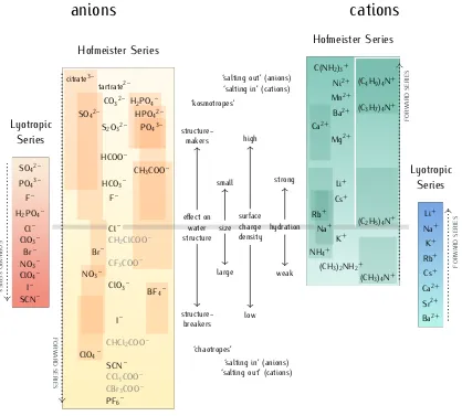
The Hofmeister and lyotropic series are depicted in Fig.1. This figure at-tempts to account for the variability seen in reports of the Hofmeister series in the literature. The ordering of ions that is highly consistent across dif-ferent studies forms the backbone of the series and is shown in the centre. The positions of other ions are indicated by a bar to show the range of po-sitions in the series that have been reported for that ion. The various dis-tinctions and adjectives that have been used in the literature to group the ions according to their behaviour (such as ‘kosmotropes/ chaotropes’) are reported in the figure as well, and apply for most ions in the Hofmeister series. An evident exception is guanidinium, C(NH2)3+, which is a poorly
2.3 terminology 13
Hofmeister Series Hofmeister Series
Lyotropic Series Lyotropic Series Cl– F– HCO3– HCOO–
CH3COO– S2O32–
CO32– tartrate2–
PO43– H2PO4–
HPO42– SO42–
citrate3–
CH2ClCOO–
CF3COO– Br–
ClO3– NO3–
BF4–
I–
CHCl2COO–
SCN– ClO4–
CCl3COO–
CBr3COO– PF6–
effect on water structure size surface charge density hydration structure-makers structure-breakers small large high low strong weak ‘kosmotropes’
‘salting out’ (anions) ‘salting in’ (cations)
‘chaotropes’
‘salting in’ (anions) ‘salting out’ (cations)
Na+ Rb+ Cs+ Li+ Mg2+ Ba2+ Ca2+ Mn2+ Ni2+ C(NH2)3+
K+
(CH3)2NH2+ NH4+
(CH3)4N+ (C2H5)4N+ (C3H7)4N+ (C4H9)4N+
Cl– H2PO4–
F– PO43– SO42–
[image:45.595.92.510.61.438.2]ClO3– Br– NO3– ClO4– I– SCN– Na+ K+ Rb+ Cs+ Ca2+ Sr2+ Ba2+ Li+
anions
cations
FORW ARD SERIES FORW ARD SERIES FORW ARD SERIES FORW ARD SERIESFigure 1: The Hofmeister and lyotropic series of ions in water. The forward direction for
each series is indicated by the corresponding arrow. For the Hofmeister ions the forward series is the one of decreasing effectiveness at precipitating proteins out of solution. For the lyotropic ions, the forward series corresponds to increasing lyotropic number. The Hofmeister series were obtained by combining those repor-ted in several references: for anions,Cacace et al.(1997),Collins and Washabaugh
(1985),Hamaguchi and Geiduschek(1962), Hanstein(1979),Kunz (2010), Kunz,
Henle et al.(2004),Maiti et al.(2009),Pinna et al.(2005),von Hippel and Schleich
(1969),von Hippel and Wong(1964),Y. Zhang and Cremer(2010) andZhao(2016); for cations,Arakawa and Timasheff (1984),Cacace et al. (1997), Carpenter and Lovelace(1935),Fischer and Moore(1907),Jain and Ahluwalia(1996),von Hippel
and Schleich(1969),von Hippel and Wong (1964) andZhao(2016). The ion is
positioned in its most agreed upon ranking, and bars indicate the variations in po-sition among different publications. The relative popo-sitioning of the haloacetates is well-known, but their positioning with respect to the ‘classic’ anions of the series is certain only in a few cases. This uncertainty is reflected by presenting these ions in grey text rather than black. The ethyl- to butylammonium cations ordering is known with respect to the tetramethylammonium ion, but not to the other cations in the series with certainty. A white line has therefore been drawn around these ions to mark the discontinuity. Ions at one end of the series are often attributed with having the opposite effect to ions at the other end of the series. As such there is a point in the series where the influence of ions reverses. The grey horizontal line traces the divide that corresponds to this property reversal. Exceptions to this classification are Rb+ and Cs+, which are larger and less hydrated than Na+and
K+; the guanidinium ion (C(NH2)3+) and the tetraalkylammonium cations which
The salting-out ability of the tetraalkylammonium series decreases from (CH3)4N+, generally a salting-out cation (although this can change
depend-ing on conditions, seeJain and Ahluwalia(1996) andvon Hippel and Wong,
1964), to (C4H9)4N+, which is a very effective salting-in agent (Jain and
Ahluwalia,1996;Mason, Dempsey et al.,2009). This behaviour is analogous to the anions series, where smaller ions are more effective salting-out agents. But the water structure-making ability of the tetraalkylammonium cations also progressively increases with the length of the alkyl chains (and therefore the cation size), due to ‘hydrophobic hydration’ (Marcus,1994;Zhao,2016), in contrast to what happens for the inorganic anions and cations. Therefore, the relationship between the size (and surface charge density) of the tetraal-kylammonium cations and their effect on water structure (and on protein stability) is the opposite of the one observed for inorganic cations. Few ac-counts of the relative positioning of the tetraethyl- to tetrabutylammonium ions with respect to the main cations of the series are available: these ions are therefore separated by a white line in Fig.1, but their positioning follows their general behaviour (Marcus,1994;Zhao,2016): (C2H5)4N+is considered
as neutral to salting-in, and (C4H9)4N+is extremely salting-in; (CH3)4N+has
generally a salting-out effect, and can be more or less potent than NH4+
de-pending on the experiment (Hyde et al.,2017).
The ordering of ions in the Hofmeister and lyotropic series is similar, but it is not identical. They are most similar for anions. Notable are the in-versions of fluoride with dihydrogenphosphate, chlorate with bromide, and nitrate and iodide with perchlorate between the series. For cations, the two series run in oppositedirections, and whereas the divalent cations ordering is mirrored from the Hofmeister to the lyotropic series, the ordering of the alkali metal cations is not: the lyotropic series follows the cation size from caesium to lithium, whereas the Hofmeister series (in its most commonly proposed order) runs as: potassium > sodium > rubidium > caesium > lith-ium. Notably, the lyotropic numbers are not available for the tetraalkylam-monium cations, and therefore these ions cannot be positioned within the lyotropic series. These distinctions between the Hofmeister and the lyotropic series will be used later in the identification of sie trends in non-aqueous solvents.
2.4 characteristics of non-aqueous solvents 15
theory of Hofmeister effects has not been achieved after more than a century from its first report.
In the ensuing chapters, we are going to also encounter cases where the ordering is ion-dependent, but neither the Hofmeister nor lyotropic series is evident, as for anions, theviscosity B-coefficients (see Bη) (vbc) (Bilaniˇcová et al.,2008;Collins and Washabaugh,1985), thelimiting molar ionic conduct-ivity (lmc) (Marcus, 2015), and for the ion pairing of tetraalkylammonium salts in ethanol (Giesecke, Mériguet et al.,2015).
In the cases where the series runs opposite to the conventional order, that have been known as either the reverse, inverse or indirect Hofmeister series, the term ‘reverse’ is employed here.
The great success of the Hofmeister series is that it is so regularly observed in systems that are very different: a great many systems adhere to the Hof-meister paradigm (Kabalnov et al.,1995;Lagi et al.,2007;Lonetti et al.,2005; Oncsik et al.,2015; Piculell and Nilsson,1989; Roberts et al.,2002;Ru et al.,
2000;Salomäki et al.,2004;Schott,1995;Vrbka et al.,2004;Washabaugh and Collins, 1986; Wiggins, 1997). The negative consequence of this is that, on occasion, observations of sie are described as Hofmeister effects when the strength of the influence of the ions does not follow the Hofmeister series, this somewhat clouds the field.
2.4 characteristics of non-aqueous solvents
Non-aqueous solvents are liquids other than water. This work is concerned with the subset of non-aqueous solvents that are capable of dissolving salts. These solvents usually have high dielectric constant in order to be able to sep-arate the charges of the electrolyte. But many other subtle and interwoven characteristics come into play to define what is a good solvent for electro-lytes: the capability of donating/accepting hydrogen bonding, the physical size of the solvent molecules, the specific chemical groups in the solvent mo-lecule that interact with the anion and the cation. Extensive descriptions are available inIzutsu(2009) andMarcus(2015).
Table 2lists the properties of the solvents included in this thesis. Among those, the empirical parameters expressing solvent acidity and basicity (do-nor and acceptors numbers) need illustration.
The Gutmann Donor NumberDNis a measure of the basicity of a solvent. It represents the ability of solvent molecules to donate a free electron pair from their donor atoms (O, N or S). It is quantified as the negative of the standard molar enthalpy of reaction −∆H−◦ of the solvent with the Lewis acid antimony pentachloride SbCl5, in dilute solution in the inert solvent
1,2-dichloroethane at 25◦C (Marcus, 2015). These values are expressed in kcal mol−1units, as a difference from the reference solvent
lit
er
at
ur
e
re
vie
[image:48.595.89.638.157.400.2]w
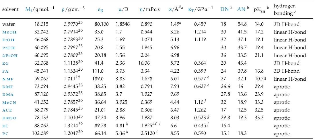
Table 2:Physical properties of the solvents investigated.
solvent Mi/g mol−1 ρ/g cm−3 R µ/D η/mPa s α/Å3a kT/GPa−1 DNb ANb pKshb hydrogen bondingc
water 18.015 0.997025 80.100 1.8546 0.890 1.49d 0.459 18 54.8 14.0 3D H-bond
meoh 32.042 0.791420 33.0 1.7 0.544 3.26 1.214 30 41.5 17.2 linear H-bond
etoh 46.068 0.789320 25.3 1.69 1.074 5.13 1.119 32 37.1 19.1 linear H-bond
proh 60.095 0.799725 20.8 1.55 1.945 6.96 30 33.7 19.4 linear H-bond
2proh 60.095 0.780925 20.18 1.56 2.04 6.98 36 33.5 21.1 linear H-bond
eg 62.068 1.113520 41.4 2.36 16.06 5.72 0.364 20 43.4 3D H-bond
fa 45.041 1.133420 111.0 3.73 3.34 4.22 0.399 24 39.8 16.8 3D H-bond
nmf 59.067 1.01119 189.0 3.83 1.678 6.01 0.577e 27 32.1 10.74 linear H-bond
dmf 73.094 0.944525 38.25 3.82 0.794 7.93 0.627e 26.6 16 29.4 aprotic
dma 87.120 0.937225 38.85 3.7 1.927 9.69 27.8 13.6 23.9 aprotic
mecn 41.052 0.785720 36.64 3.925 0.369 4.44 1.10f 32 18.9 33.3 aprotic
ace 58.079 0.784525 21.01 2.88 0.306 6.47 1.262 17 12.5 32.5 aprotic
dmso 78.133 1.101025 47.24 3.96 1.987 8.03 0.523g 29.8 19.3 33.3 aprotic
ec 88.062 1.321439 89.78 4.81h 1.92540i 6.6 0.435j 16.4 aprotic
pc 102.089 1.204720 66.14 5.36h 2.5120i 8.55 0.590 15.1 18.3 aprotic Data from the CRC Handbook of Chemistry and Physics (Lide,2010), unless otherwise noted.
Mi: molar mass;ρ: density at thetin◦Cindicated by the superscript;R: dielectric constant;µ: dipole moment;η: viscosity at25◦C;α: experimental
static polarisability; kT: isothermal compressibility at20◦C;DN: electron pair donicity (Gutmann donor number); AN: (Gutmann-Mayer acceptor number); pKsh: solvent autoprotolysis constant.
aBosque and Sales,2002;bIzutsu,2009;cJenkins and Marcus,1995;dWeiss et al.,2012;eEasteal and Woolf,1985;f Easteal and Woolf,1988;gMarcus and
2.5 methodology 17
The hydrogen bond donicity and electron pair acceptance of a solvent is correlated to its capability to contribute protons for hydrogen bonding. It is therefore limited to protic and protogenic solvents (solvents with a methyl group adjacent to a C –– O, C –––N, or NO2 group). The Gutmann–Mayer
ac-ceptor numbersANof a solvent (Lewis acid) are evaluated from thenuclear magnetic resonance (nmr) chemical shift of the 31P atom of triethylphos-phine oxide Et3P –– O in dilute solution in the solvent of interest. The AN
values are dimensionless numbers, the higher the number, the higher the solvent acidity (Marcus,2015).
Other scales have been defined, such as the solvent acidity scales are Kosower’s Z values, Dimroth and Reichardt’s ET scale, Kamlet and Taft’s
αKTparameter. conversely, solvent basicity scales include Kamlet and Taft’s
βKTparameter (Izutsu,2009).
The combination of properties of these solvents is very diverse. Based on the combinations of some of the properties general classifications have been introduced (Izutsu,2009), which are not adopted here.
2.5 methodology
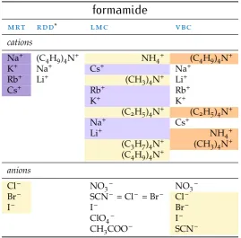
In the ensuing sections, a range of studies intosiein non-aqueous solvents are presented, grouped by solvent, and the sie trends that emerge are dis-cussed. It is immediately apparent thatsieare as ubiquitous in non-aqueous solvents as they are in water.
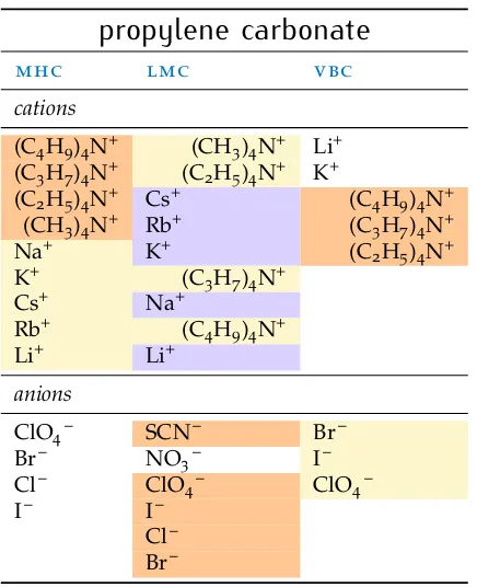
For each study the observed trend of sie for the cations and anions has been extracted and displayed in a colour-coded table to assist in the inter-pretation of the data. The order of each table column runs from largest value at the top to smallest at the bottom. The series are compared to those defined in Fig. 1. A pale yellow cell background indicates a forward Hof-meister series, orange a reverse HofHof-meister series, lilac a lyotropic series and purple a reverse lyotropic series. No colour is used where a series does not follow either the Hofmeister or lyotropic series. Where an individual ion is not included in the colour scheme for a particular series, this indicates that this ion is not in its correct location in the series. In some columns, the ammonium cation and the tetraalkylammonium cations (NH4+, (CH3)4N+,
(C2H5)4N+, (C3H7)4N+, (C4H9)4N+), which I will collectively refer to as the
‘ammonium class’ in the discussion, are offset to the right, so that they may be easily considered separately from the alkali metal cations. This has been done as these two classes of cations show consistent behaviour when con-sidered separately but not an overall trend when concon-sidered together.
Table 3:Trends in sieobserved in water. Data fromMarcus(2015).
water
mrt rdd* mhc lmc vbc
cations
Li+ Li+ (C
4H9)4N+ Rb+ (C4H9)4N+
Na+ Na+ (C
3H7)4N+ Cs+ (C3H7)4N+
K+ (C
4H9)4N+ (C2H5)4N+ NH4+ (C2H5)4N+
NH4+ (CH3)4N+ K+ Li+
Li+ Na+ (CH
3)4N+
Na+ (CH
3)4N+ Na+
K+ Li+ NH4+
Rb+ (C2H5)4N+ K+ Cs+ (C3H7)4N+ Rb+
(C4H9)4N+ Cs+
anions
F– ClO
4– SCN– = ClO4– SO42– HPO42–
SO42– I– F– CO32– H2PO4–
Cl– Br– I– Br– CO32–
Br– Cl– Cl– Cl– CH3COO–
NO3– Br– I– SO42–
I– NO3– F–
ClO4– Cl–
SCN– SCN–
HPO42– Br–
F– NO3–
HCOO– HCOO–
CH3COO– ClO4– H2PO4– I– *from electrolytes, ionic values not available.
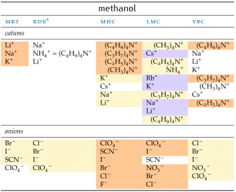
• Thenmrmolecular reorientation time (mrt)of the solvent in the
pres-ence of ions, calculated as the ratioτs(i) or/τsor, of the molecular
reori-entation time constant in the presence of ions to the time constant of the neat solvent.
• The relative limiting static dielectric decrement (rdd) of an ion
solu-tion as its concentrasolu-tion approaches zero, calculated as the ratio of the limiting static dielectric decrement caused by the ion to the relative per-mittivity of the pure solvent−δ(i)/εs(ce→0), with units dm3mol−1.
• The constant pressure standard partial molar heat capacity of the ion
(mhc),C∞pi inJ K−1mol−1 which is the difference between the specific
heat of the solution of the ion and that of the pure solvent, in the limit of infinite dilution.
• Thelimiting molar ionic conductivity (lmc)λ∞i (S cm2mol−1).
2.6 Methanol 19
Table 4:Trends in sieobserved inmeoh. Data fromMarcus(2015).
methanol
mrt rdd* mhc lmc vbc
cations
Li+ Na+ (C
4H9)4N+ (CH3)4N+ (C4H9)4N+
Na+ NH
4+= (C4H9)4N+ (C3H7)4N+ Cs+ Na+
K+ Li+ (C
2H5)4N+ (C2H5)4N+ Li+ (CH3)4N+ NH4+ K+
K+ Rb+ (C
3H7)4N+
Cs+ K+ (CH
3)4N+ Na+ (C3H7)4N+ Cs+
Li+ Na+ (C2H5)4N+ Li+
(C4H9)4N+
anions
Br– Cl– ClO
4– ClO4– Cl–
I– Br– SCN– I– Br–
SCN– I– I– SCN– I–
ClO4– ClO4– Br– NO3– NO3–
Cl– Br– ClO4–
F– Cl–
*from electrolytes, ionic values not available.
This table is an important point of comparison for the measurements made in non-aqueous solvents. In fact, some of these measurements follow a known series and therefore are of particular interest.
It must be noted that water is somewhat soluble in all the non-aqueous solvents and its presence may have some influence on the experimental res-ults. The degree to which water has been excluded is not apparent in many of the studies and therefore cannot be addressed here.