THE QUANTUM MECHANICS
OF
ELECTRO-OPTIC FEEDBACK,
SECOND HARMONIC GENERATION,
AND
THEIR INTERACTION
Matthew Scott Taubman
B.Sc.(Hons), The Australian National University, 1989.
A thesis submitted for the degree of Doctor of Philosophy
of The Australian National University.
D e c la r a tio n
The contents of this thesis are entirely my own work except where
indicated.
To my late father,
A ck n ow led gem ents
I would like to take this opportunity to sincerely thank my supervisors Dr Hans Bachor and Dr David McClelland for the continual support, guidance and understanding they have given me during my PhD. I would also like to thank Dr Craig Savage, Dr Mark Andrews and Dr Gerard Milburn for guidance and useful discussions.
A big thank you is owed to my colleagues. Although a PhD is essentially ones own work, I could not have achieved half as much without the interaction with the rest of the group. In particular, I would like to thank Andrew White, Tim Ralph, Ping Koy Lam, Charles Harb and Mai Gray for sharing their expertise with me. A special thank you is owed to Andrew and Ping Koy for helping me with the printing and binding of this thesis.
Any experimental PhD would be very difficult without the support of a me chanical workshop. Many thanks to Graham Pike and the workshop staff for the various jobs they have done for me over the years. My special thanks go to Brett Brown whose willingness to fabricate often complicated and ill-conceived mechanical bits and pieces on very short notice is most appreciated. During my PhD I have had the opportunity of working with several electronics workshop staff. I wish to extend my thanks to them all, as each of them have contributed to my achievements. I have also greatly enjoyed their companionship. They include: Dave Cooper, Alex Eades, Doug Crawford and Walter Goydych. I would also like to thank the general staff for the support throughout the years, in particular Felicity Davey who always seemed to know exactly what to do to solve any administrative problem.
A b stract
C on ten ts
1 I n tr o d u c tio n 1
1.1 What is squeezing?... 1
1.2 How is squeezing p ro d u c e d ? ... 4
1.3 Experimental h is to r y ... 5
1.4 Feedback, and the goals of the project ... 7
1.5 Thesis stru c tu re ... 9
2 T h e o ry ; b a ck g ro u n d , d e fin itio n s and to o ls 10 2.1 Summary and Introduction... 10
2.2 N om enclature...10
2.3 Basic quantum optics and squeezing... 12
2.3.1 Electromagnetic fields, the simple harmonic oscillator and Fock states ...12
2.3.2 Coherent s t a t e s ... 14
2.3.3 The uncertainty principle, minimum uncertainty states and q u a d ra tu re s ... 18
2.3.4 Squeezed s t a t e s ... 22
2.3.5 Intensity squeezing vs quadrature sq u e e z in g ...26
2.3.6 Representation of modes, and lin earisatio n ... 27
2.3.7 Taking the Fourier transform ...28
2.3.8 Deriving spectra ...28
2.4 Simple Cavity S y s te m s...29
2.4.1 The equations of motion, input and o u tp u t... 29
2.4.2 Relating the coupling rates to experimental parameters . . . . 32
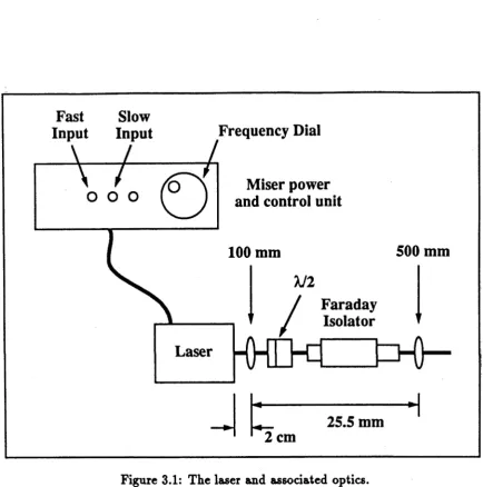
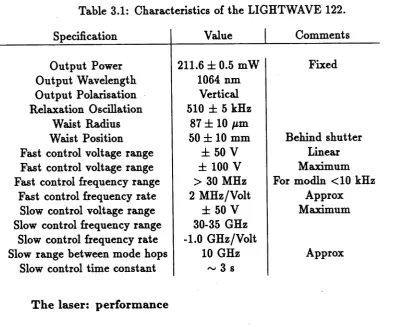
3 E x p e r im e n ta l te c h n iq u e s and d e ta ils 38 3.1 The laser and associated optics ... 38
3.2 Electro-optic m o d u lato rs...43
3.3 General o p tic s ... 44
3.4 Detectors ... 44
3.5 Amplifiers and signal g en erato rs...47
3.6 The spectrum a n a ly s e r... 47
3.7 Splitter-combiners, mixers, a tte n u a to r s ... 47
3.8 Locking the laser, mode cleaner and S H G ... 47
3.9 The UNIPID5.0 locking circu it...54
3.10 The miser controller ... 59
3.11 The mode cleaner P I D ... 63
4 T h e sim p le feed b a ck lo o p 66 4.1 Summary, Introduction and H isto ry ...66
4.2 T h e o ry ... 68
4.3 E xperim ents...82
4.4 R esu lts... 87
4.5 Discussion and Conclusions ... 93
5 T h e la ser and m o d e clea n er 96 5.1 Summary and Introduction...96
5.2 T h eo ry ...97
5.2.1 The laser ... 97
5.2.2 The Mode C l e a n e r ... 105
5.3 The design of the mode c le a n e r ...I l l 5.4 Experiment and R e s u l t s ... 112
5.5 Discussion and C onclusion... 116
6 S e c o n d h a rm o n ic g e n e r a tio n 118 6.1 Summary and introduction...118
6.2 The semi-classical equations, intuitive ideas ... 119
6.3 Singly resonant SHG t h e o r y ...121
6.3.1 Limiting case s... 126
6.3.2 Before modelling the experim ent... 129
6.4 The design of the second harmonic generator cry stal...132
6.5 Experiments and R e su lts... 133
6.5.1 Experimental arrangement ... 133
6.5.2 Performance... 135
6.5.3 Experimental squeezing s p e c t r a ... 136
6.5.4 Further Im provem ents...140
6.5.5 Comparison to theory ... 146
6.6 Discussion and C onclusion... 151
7 C o m b in in g S H G and feed b a ck 152 7.1 Summary and Introduction... 152
7.2 Theory of electro-optic squeezing tran sfe r...153
7.2.1 The simple feedback lo o p ... 153
7.2.2 Feedback on singly resonant S H G ...154
7.3 Experiments and r e s u l t s ... 162
7.3.1 Simple feedback experimental arrangem ent... 162
7.3.2 Results of simple feedback loop tran sfer... 164
7.3.3 Comparison to the theoretical predictions ... 164
7.3.4 Cross-colour feedback experiments...166
7.4 Discussion and Conclusions ... 173
8 C o n clu sio n 175 8.1 R eview ... 175
8.1.1 Electro-optic feedback system s...175
8.1.2 Second harmonic g e n eratio n ...176
8.1.3 The interaction of electro-optic feedback and S H G ... 177
8.2 General conclusions... 178
8.3 Further work ... 178
List o f Figures
1.1 Phasor diagram of coherent and squeezed states... 3
2.1 Probability distribution for the vacuum state...15
2.2 Phasor diagrams comparing squeezed states and various other states. 22 2.3 Transition from coherent state to number state... 24
3.1 The laser and associated optics... 39
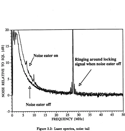
3.2 Laser spectra, noise tail ... 41
3.3 Schematic for photodetectors... 46
3.4 Locking apparatus for the SHG experiments... 52
3.5 Locking apparatus for the improved SHG experiments...53
3.6 Picture of dither trace while locked... 54
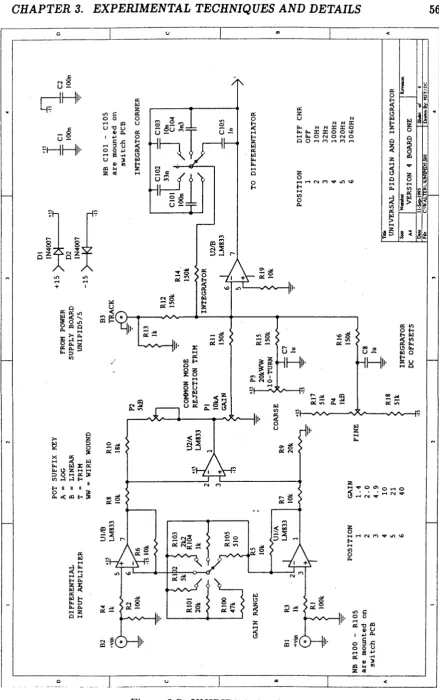
3.7 UNIPID5.0 circuit part i... 56
3.8 UNIPID5.0 circuit part ii... 57
3.9 UNIPID5.0 circuit part iii... 58
3.10 Miser Fast controller... 60
3.11 Miser Slow controller... 61
3.12 Miser Controller Power supply...62
3.13 The mode cleaner PID circuit...64
4.1 Schematic of feedback loop showing optical fields...70
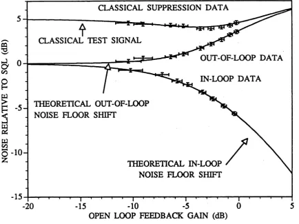
4.2 Noise floors and classical signals...76
4.3 Schematic of feedback loop used for main experiments...83
4.4 Full apparatus for main feedback experiments... 84
4.5 Schematic for direct in-loop modulation...86
4.6 Schematic for out-of-loop homodyne measurements. ... 87
4.7 Typical experimental photocurrent spectra... 89
4.8 Response to varying gain; experiment vs theory... 90
4.9 Out-of-loop noise floor vs beam splitter ratio... 91
4.10 Homodyne out-of-loop measurements...92
5.1 Cascaded formalism and the flow of noise... 98
5.2 Energy level diagram showing operation of the laser...99
5.3 Theoretical curves showing the relaxation oscillation of the laser. . . . 104
5.4 Diagram of the mode cleaner showing the various fields... 106
5.5 Theory plots of transmitted and reflected spectra of the mode cleaner. 110 5.6 Arrangement of laser and mode cleaner for recording their spectra. . . 113
5.7 Picture of a resonance sweep of the mode cleaner...114
5.8 Experimental and theoretical spectra for the laser and mode cleaner. 115 6.1 Theoretical amplitude and phase spectra of SHG... 127
6.2 Diagram of the monolithic crystal... 132
6.3 SHG experimental arrangement...134
6.4 Picture showing thermal bistability seen in the crystal... 137
6.5 Experimental squeezing spectra without the mode cleaner...138
6.6 Experimental squeezing spectra with the mode cleaner... 139
6.7 Experimental spectrum of transmitted light, without mode cleaner. . 140
6.8 Improved SHG experimental arrangement... 141
6.9 Squeezing spectra of improved SHG experiment with the mode cleaner. 143 6.10 Reliability plus and minus traces...144
6.11 Squeezing on the reflected fundamental...145
6.12 Inferred squeezing from SHG experiments, and theory curves... 148
6.13 Inferred squeezing from improved SHG experiments, and theory curves. 149 7.1 Squeezing transfer using simple feedback loop...155
7.2 Schematic of SHG feedback system using frontal modulation... 158
7.3 Green-green feedback transfer experiment... 163
7.4 Feedback transfer results... 165
7.5 Transmitted (out-of-loop) spectra... 168
7.6 Cross-colour correlation experiment...169
7.7 Correlation spectra...170
7.8 Correlation difference traces...171
List of Tables
2.1 Comparison of models...36
3.1 Characteristics of the LIGHTWAVE 122... 40
3.2 Electro-optic modulators listed under their uses... 43
3.3 General Optics... 45
3.4 Amplifiers and signal generators...48
3.5 Minicircuits Components...48
5.1 Mode cleaner mirror parameters...112
5.2 Mode cleaner powers; theory vs experiment...115
6.1 SHG and laser parameters to fit theory and experiment... 150
To th e read er
The PhD project which I undertook was certainly mostly experimental. How ever, I have always wanted an understanding of the theory, but perhaps from a different point of view to the theorist. I have been rigorous where I have felt it nec essary to understand the theory rigorously, and intuitive where I thought it might be more useful, especially for the experimentalist who might read this thesis. To this end I have included chapter 2 which covers the basics of quantum optics as I view them, and compares the way theoreticians and experimentalists view cavity systems.
As the title of my thesis suggests, my PhD consists of research in a number of areas. Because of this, there is no main theory chapter or main experimental chapter covering all my work. Chapters 4 to 7 each deal with a specific area of research; the simple feedback loop, the laser and mode cleaner, the second harmonic generator, and finally, feedback applied to second harmonic generation. Each of these chapters contains the relevant theory, experimental descriptions, results and conclusions. In this manner, they form the core of my thesis. The remaining chapters such as introduction, conclusion and background chapters while not following this structure, form the platform upon which this core is built.
C hapter 1
In tro d u ction
1.1
W hat is squeezing?
Since the 1920’s the implications of Heisenberg’s uncertainty principle regarding measurement have been well known; that is, one cannot measure to arbitrary accu racy both the position and momentum of a particle. This is because at this level of accuracy our act of measurement to ascertain the value of either variable disturbs the other in a random manner. Thus if the position and momentum of a large en semble of particles are measured, two distributions will be obtained, the widths of which when multiplied will give a product which can never be less than a specific value. Such pairs of variables are referred to as conjugate variables. Similarly, this limitation also applies to measurements of the characteristics of light for the very same reason. If the intensity (or photon number) and phase1 fluctuations of an opti cal electromagnetic field are measured, distributions are obtained which also give a minimum product. This is because, the energy in the field seems to exist in discrete packets or quanta, called photons.
The first evidence of this optical quantum phenomenon was found in 1900, when M. Planck saw that by postulating that light be “quantised”, a nasty dis agreement between experiment and theory could be completely resolved - namely the ultraviolet catastrophe. This led to the famous and now widely used “black body distribution”, or “black body curve”. In 1905, Einstein explained the photoelectric effect by assuming light to be composed of individual quanta. Electrons optically released from a cathode in a vacuum tube using a narrow-band light source, have a specific energy. The value of this energy depends purely on the frequency of the light and the amount of energy required to free the electrons (work function). It does not depend on the intensity of the light. This is because the light can only impart
lrrhe definition of a quantum mechanical phase is a contentious issue. [1, 2]
CHAPTERl. INTRODUCTION 2
energy to the electrons in bundles of a specific size, this size being proportional to the frequency of the light.
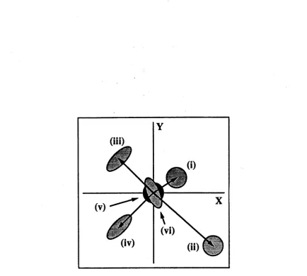
The significance and impact of this phenomenon is that the limitation to the accuracy of measurements in intensity or phase of an optical field results in a noise floor, which when first discovered, seemed unsurpassable. It is not a function of the detection process, and hence further refinements to photodiodes or measurement apparatus make no difference. This floor is known as the “quantum noise floor” (QNF) or “standard quantum limit” (SQL). If instead of examining the fluctuations or noise in the intensity and phase of an optical field, we examine the in-phase and out-of-phase fluctuations of the field amplitude, known as “quadratures”, then in general, states of light which are at the SQL exhibit equal noise in both of these quadratures. We can represent these states on a phasor diagram as a circle some distance from the origin, depicted by (i) and (ii) in Fig. 1.1. The distance from the origin represents the mean amplitude of the state, and the circle represents the uncertainty in the position of the phasor. They are called coherent states, and their photon statistics are Poissonian. However, it has been known for some time that the noise in one of the conjugate variables can be reduced at the expense of allowing more noise in the other. This produces a state of light, known as a squeezed state, [3, 4, 5] depicted by states (iii), (iv) and (vi) in Fig. 1.1. The term squeezing refers to the deforming of the circle into some other shape, usually an ellipse. An amplitude quadrature squeezed state has “sub-Poissonian” photon statistics, and when incident on a detector gives rise to a noise floor lower than the SQL. Hence it could be used to make optical measurements of small signals with better signal to noise ratio than otherwise possible.
CHAPTER 1. INTRODUCTION 3
Figure 1.1: Ph&sor diagram of coherent and squeezed states.
[image:15.559.76.511.60.450.2]CHAPTER 1. INTRODUCTION 4
1.2
H ow is sq u e e z in g p ro d u ced ?
There are in general two ways of producing squeezed light; produce the light in a squeezed state to begin with, or use some sort of non-linear process to generate squeezed light from coherent or even noisy light.
The first method, that of making the light squeezed to begin with, includes the use of high quality laser diodes, driving them high above threshold and thus with high quantum efficiency, with a very quiet drive current. Electrons in a wire, can be made to flow with a sub-Poissonian statistical distribution simply by using a high resistance in series with a large drive voltage. In a laser diode with near unity quantum efficiency, such a current can be made to produce a stream of photons which is also sub-Poissonian, thus constituting an amplitude-squeezed output. [6] In theory, squeezed light can also be produced using rate-matching. [7, 8, 9] If several cascaded transitions in a laser system have similar decay rates, then amplitude squeezed output can result if the pump transition is also matched. This is because the continual cycling of the atomic electrons through each energy level at the same rate has a regularising effect, resulting in noise reduction of the light produced from the lasing transition.
The second method, that of using a non-linear technique to transform a coher ent state into a squeezed state has several possibilities. One is to use a non-linear process which will introduce some correlation between the fluctuations in the am plitude and phase of the optical field. This is a third order non-linear process. An example is the Kerr effect, in which the refractive index of a medium is intensity dependent. Consequently, a fluctuation in the intensity induces a corresponding one in the phase of the field. At low photon numbers this causes a skewing of the circle in the phasor diagram into a “tear” shape, called a Kerr state. [10] At higher photon numbers, this becomes an ellipse but it is neither a quadrature amplitude or quadrature phase squeezed state. Another possibility is to use a non-linear pro cess to amplify or attenuate one quadrature (and thus the fluctuations in it) with respect to the other. This is a second order non-linear process and is the basis for optical parametric oscillation, and its reverse process, second harmonic generation, the latter of which will be dealt with in great detail in this thesis.
CHAPTER 1. INTRODUCTION 5 made resonant with any atomic transition as such, but the crystal must be held at certain temperatures and the light incident at certain angles to effect phase match- ing. [11]
1.3
E xperim ental history
There have been many squeezing systems developed in theory over the last 15 years, but despite this, relatively few experiments have been successfully performed. This may be an indication of how difficult it is in practise to produce squeezed states of light. What follows here is a summary of the most significant experiments which have been performed so far.
The first experimental squeezing was achieved by Slusher et al in 1986 [12] and 1987 [13] using nondegenerate four-wave mixing. A continuous wave (cw) ring laser was used to drive an optical cavity. A beam of sodium atoms passing trans versely through the cavity interacted with the cavity mode, and thus quadrature squeezed vacuum was produced inside the cavity via the four wave mixing process. In 1986, 7% to 10% squeezing was observed. In 1987, this was increased to 20%. The best squeezing in atomic media was obtained by workers in Kimble’s group in 1987; Raizen et al [14] and Orozco et al [15], observing 30% vacuum squeezing in a coupled atom-cavity system. After propagation losses and detector inefficiencies were accounted for, the inferred squeezing was 53%. Hope et al [16] at the ANU in Canberra observed bright squeezing with a noise reduction of 18% in a near-bistable atom-cavity system, the inferred level being 50%.
Squeezing has also been obtained using solid state media, such as second har monic generation (SHG) crystals and optical parametric oscillators (OPOs). The first of these successful experiments was done in 1987 by Wu et al [17] using a sub-threshold OPO. A quadrature squeezed vacuum, with greater than 60% noise reduction was observed. The inferred squeezing from this measurement is more than ten-fold, ie, greater than 90%. It was also shown that the squeezed state obtained was also a minimum uncertainty state.
CHAPTER 1. INTRODUCTION 6
on the fundamental for short time intervals, also in a doubly resonant system, but this time using a cavity system where the mirror coatings were placed directly on the crystal. (This is referred to as a monolithic crystal.)
Towards the middle of my post graduate studies, workers at Konstanz in Ger many [21] reported successful squeezing experiments using a singly resonant mono lithic doubler. Previously it had been thought that it was necessary to be near an instability point to observe squeezing. Since this is far from true in singly resonant systems, the possibilities had not been previously investigated. In reference [21], Collett demonstrated good squeezing to be possible in singly resonant systems, and the accompanying experiments demonstrated an observed squeezing of around 20 % on the second harmonic (inferred squeezing of 30 %).
In 1995 Taubman et al [22] at ANU demonstrated an observed squeezing on the second harmonic of 25% (inferred 40%) obtained by using a mode cleaning cav ity placed between the laser source and the second harmonic generator to reduce the leiser noise and expose regions of squeezing which had been previously masked. In this thesis these results are discussed as well as showing improvements, the lat est observed squeezing on the second harmonic being 27% (inferred squeezing of 42%). Unlike previous experiments [21], agreement between theory and experiment is excellent, as models were developed which included the noise character of the laser. [22, 23]
In 1986 the first squeezing in an optical fiber was obtained by Shelby et al [25] achieving 12%. Here a fiber was cooled to below 4.2 degrees Kelvin and driven by a Krypton-ion laser. Forward nondegenerate four-wave mixing was used to produce squeezing.
Experiments have also been performed in which the light was squeezed upon generation. Space-charge-limited vacuum tube experiments (Frank Hertz experi ment) which have been seen to produce squeezing due to the natural tendency of electrons to repel one another and become a sub-Poissonian distribution. Highly efficient light emitting diodes and laser diodes driven from highly regulated current sources as mentioned earlier, have also been seen to produce squeezing. Examples include Tapster [26], 4% reduction, Rottengatter [28], 28%, and Edwards [29], 30%, the figures being the observed (not inferred) noise reduction in each case.
Electro-optic feedback techniques have been used to generate sub-Poissonian photocurrents. Experiments include Machida and Yamamoto [30] in 1986, Machida
exper-CHAPTER 1. INTRODUCTION 7 iment, a laser diode formed part of a negative feedback loop which was used to reduce amplitude noise of the feedback loop photocurrent. 7 dB or 75% reduction in the noise power spectrum of the photocurrent was observed. While the fields produced by these experiments may be squeezed, they are not useful since they are not extractable. This topic is dealt with in detail in this thesis.
Another type of non-classical light experiment is twin photon beam production. This occurs in an 0 P 0 crystal, in which a single photon is down-converted to two photons of double the original wavelength, half the energy. The two resulting beams of light which may not be squeezed on an individual basis, together represent a non-classical state of light. This is because the photons occur in correlated pairs, one in each beam. Information can be obtained about the photons in one beam without affecting them, simply by detecting or measuring some property of the photons in the correlated beam. An example of such an experiment is that of Heidmann et al [34], who in 1987, observed a 30% noise reduction in the correlation between the twin beams of an OPO, compared to that of two uncorrelated Poissonian beams. A usable squeezed output from these systems has been generated by applying electro-optic feedback to twin beam generators. In this manner, one beam can be sacrificed on a photodetector to derive information about the amplitude fluctuations on the other correlated beam. This allows the noise on the second beam to be reduced by feeding the signal derived from the first, to an amplitude modulator either placed in the pump beam to the OPO (feedback) or in the second output beam (feedforward). [35, 36]
1.4 Feedback, and the goals of the project
CHAPTER 1. INTRODUCTION 8
will always be so, regardless of how much negative feedback is applied.
However, there is a potentially exciting and useful possibility of this theorem. If one begins with a sub-Poissonian beam, specific levels of positive feedback are predicted to move the noise level of the field extracted from an electro-optic feedback loop away from the Poissonian limit, making it even more sub-Poissonian. This implies that electro-optic feedback could be used to make an already squeezed output of a system even more squeezed, but only if there is another correlated squeezed output beam to use as a feedback source. This latter constraint means that this idea cannot be used to make a source which produces a single beam more squeezed than it would be without feedback. It does however, imply that squeezing can be
transferred between two correlated squeezed beams. To demonstrate this was the major goal of my project.
In addition to this, there were two other goals. Firstly, a thorough under standing of the behaviour of electro-optic feedback systems when operating near the quantum limit was to be attained. Secondly, a reliable and stable squeezed source was to be built and modelled. At this time, our group had access to the material and the technology for building OPOs and second harmonic generators (SHGs). We chose to build an SHG as a squeezed source rather than an 0 P 0 , because SHG provided sufficient opportunities to test the electro-optic transfer of squeezing, and an 0 P 0 required the construction of an SHG as a first step. In addition, recent advances in the fabrication of monolithic cavity systems [24] had allowed co-workers overseas [21] to build SHGs which produced extremely reliable squeezing. While OPOs were known to develop much larger squeezing, the same reliability had not at that time been demonstrated.
CHAPTER 1. INTRODUCTION 9 the second harmonic, and the auxiliary fundamental beams. As in the case of green- green feedback, cross-colour feedback could be performed with the modulator placed in the output beam onto which squeezing was to be transferred, or in the pump beam before the SHG.
1.5
T hesis structure
C hapter 2
Theory; background, d efin ition s
and to o ls
2.1
S u m m a ry an d In tr o d u c tio n
This chapter is aimed at the graduate experimentalist, and apart from the first section which discusses the notation used throughout this thesis, can be skipped or only glossed over by people well versed in the theory of quantum optics. The basics of the quantisation of the electromagnetic field are covered, number, coherent and squeezed states are discussed, and the representations of cavity modes, coupling cavity systems to the external environment and finding spectra are addressed. For more information on these topics the reader is directed to reference [2]. In particular, chapters 6 and 7 of this reference give an in-depth study of stochastic methods and the input/output formulation of optical cavities respectively. Finally, a discussion on relating the coupling rates used in the equations of motion for cavity systems to the everyday experimental parameters such as reflectance and loss is undertaken. This part is necessary knowledge for the experimentalist who is just beginning to grapple with the theory, and comparing the two. [39]
2.2
N o m e n c la tu r e
In this thesis I will use certain character sets to represent various classes of quanti ties, and particular characters for specific reoccurring quantities. These are defined below. All pronumerals in this work will follow these conventions unless otherwise specifically stated. I will begin this list of definitions however, with those things which I do not do.
1. Operators are not represented by a “hat”, for example a .
CHAPTER 2. THEORY; BACKGROUND, DEFINITIONS AND TOOLS 11
2. Explicit time or frequency dependence will not be shown anywhere unless it is absolutely necessary to avoid confusion. Most non-constants which arise will be time dependent, with the exception of those which have a “tilde” above them, for example A, which are frequency dependent.
The general definitions follow.
1. 6 is reserved specifically for “a small change in ...” 2. £ is reserved for beam splitter intensity transmission. 3. 9 is reserved for modulator amplitude transmission. 4. k is reserved for cavity coupling rates.
5. 7 is reserved for decay rates for atomic energy levels. 6. fi is reserved for non-linear loss coefficient.
7. v, f are reserved for frequencies measured in Hertz. 8. is reserved for frequency in radians per second.
9. The first two lower case Arabic characters, a, 6, will represent the annihilation operators, and thus the amplitudes, of the modes of cavity systems. The conjugate of an operator will be denoted by a dagger, for example, a —> a \
10. The semi classical values of these modes will be represented by the correspond ing Greek character, and these particular Greek letters are reserved for this purpose. The semi-classical value of a conjugated operator is represented by the complex conjugate of the corresponding Greek letter, being represented by an asterisk.
CHAPTER 2. THEORY; BACKGROUND, DEFINITIONS AND TOOLS 12 11. Upper case Arabic characters, for example, A, B, will represent field operators
other than cavity modes. This includes all input and output field operators to cavity systems.
12. The semiclassical values of these fields will be represented by the same letter with a “bar” placed over the top, for example,
A —►A
B B
13. Caligraphic script S will denote energy, and T will denote Fourier transform.
2.3
B a sic q u a n tu m o p tic s an d sq u e e zin g
2.3.1
E lectrom agnetic fields, th e sim ple harm onic oscillator
and Fock sta tes
We shall begin our discussion of the theory with a version of the classical electro magnetic field as a function of position r and time t.
E (r,t) = - a> K r ) ^ ‘1 t2-1)
where Uj(r) contains polarisation and spatial phase information.
In this expression, aj and a*■ are complex numbers. To quantise the field, we transform them to mutually adjoint operators. These obey the boson commutation relations, [a,-, a*] = 0, [a},a£] = 0 and [aj,a[] =
6jk-The energy in the electromagnetic field is given by the Hamiltonian
H = i Je(„E2 + m<)H 2) dt
which can be shown to simplify to
H = h(x>k{a\ak + i ) (2.2)
k 1
CHAPTER 2. THEORY; BACKGROUND, DEFINITIONS AND TOOLS 13
Let us now consider a single mode, and revise the basics of the SHO. The Eigenstates of the SHO are the “Fock” or “number” states |n). The number operator is N = a^a, and thus
N\n) = n\n)
Note that the number states form a complete orthonormal set. Thus any state can be expanded uniquely in terms of the number states.
(n\m) = 6nm
J2
l n ) ( n l = 1 ( 2 - 3 )n= 0
The operators a and a* are the annihilation and creation operators for the mode respectively. Their commutator is one of the most important in quantum mechanics as it is often gives rise to the differences between quantum and classical expressions.
[a, a*] = 1 (2.4)
These operators add and subtract a single photon from the mode thus:
a\n) = y/n \n — 1) a*|n) = \/n -f 1 |n + 1)
Note that the annihilation operator applied to the ground state gives zero.
a|0) = 0 (2.5)
The Hamiltonian is
H — hu>(a^a -f - )
=
f^(N + \)
CHAPTER 2. THEORY; BACKGROUND, DEFINITIONS AND TOOLS 14
H\n) = £„\n)
= ftw(n + -)|n>
The most important thing to notice about this is that the ground state energy is not zero.
So= - h u )
z
This is one of the hall-marks of quantum mechanics and in fact allows the existence of the subject m atter for this thesis itself. The ground state energy of a quantum mechanical electromagnetic field is non-zero. Thus the vacuum has energy. In fact, oddly enough, because there is no upper limit to the frequency of the modes, Eqn. (2.2) shows it has infinite energy! However, since no practical experiment has ever been able to measure absolute energy, but rather only changes in energy, there is no problem. Even though the average field of this state is indeed zero, the fluctuations in it are definitely non-zero. Hence the vacuum state incident on a beam splitter mixes its own fluctuations in with those of the other fields, causing observable effects in photocurrents and spectra.
2.3.2
Coherent sta tes
Coherent states are important because they are the closest thing theory has to a laser output when the laser is stabilised and driven well above threshold. Here we will examine the character of these states, and later in section 2.3.4, their closely related cousins, the squeezed states. We begin our discussion with the ground state |0) because although presented above as a number state with n = 0, it is unique in that it can also be thought of as the lowest level coherent state, the closest thing theory has to “nothing”.
CHAPTER 2. THEORY; BACKGROUND, DEFINITIONS AND TOOLS 15
Y
r. '
5 . V :...
“ • » * * .
• . .
- *
•• •• •
* i * ,
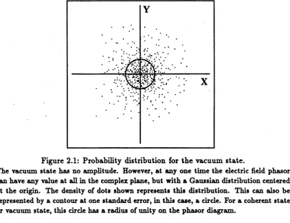
Figure 2.1: Probability distribution for the vacuum state.
The vacuum state has no amplitude. However, at any one time the electric field phasor can have any value at all in the complex plane, but with a Gaussian distribution centered at the origin. The density of dots shown represents this distribution. This can also be represented by a contour at one standard error, in this case, a circle. For a coherent state or vacuum state, this circle has a radius of unity on the phasor diagram.
This representation is simplified by using a circle centered on the origin. This circle is a contour of one standard error for the probability distribution.
The easiest way to think of a coherent state is as a shifted vacuum state. That is, shift the circle to some point a distance a away from the origin. This has now given the electromagnetic field some complex amplitude a . This is achieved in theory using the “unitary displacement operator” defined below. (For more discussion on the nature of the displacement operator see references [2, 40, 41].) This operator moves a state in phase space without changing any other attributes.
D(a) = e“ ' - “' “
Thus for the purpose of this thesis, we can define the coherent state |a) as the displacement operator D(a) acting on the vacuum state as written below.1
|a) = D(a)|0) (2.6)
We now briefly investigate the properties of the displacement operator. Using Eqn. (2.4) and the Baker-HausdorfF relation
[image:27.559.83.506.53.377.2]CHAPTER 2. THEORY; BACKGROUND, DEFINITIONS AND TOOLS 16
e ( A+B) _ e A e B e -[A, B]/ 2
we have th a t
D(a) = e -l<*l, / Je“0,e " “ ‘a
£>*(<*) = e|a|,/2e“ ‘*e~“ '
Thus
D ( a ) D \ a ) = eaate - a *°ea *ae - aat
= eaate_aat
= 1
Therefore we have th a t
(2.7)
D ~ \ a ) = £>*(<*)
which proves th a t D(a) is unitary. Similar calculations give
(2.8)
D ^ a ) = D ( - a )
D \ a ) a D ( a ) = a + a
D' ( a ) a 'D ( a ) = a* + a"
We discover som ething else about th e coherent states if we look more closely
at th e action of th e displacem ent operator, namely, their expansion in term s of the
num ber states.
But
I>(o)|0) = e-W’/*e“ V « '*|0)
e - “ ’a |0> 1 — a* a H—— a 2 + • ..
10
}
CHAPTER 2. THEORY; BACKGROUND, DEFINITIONS AND TOOLS 17 So
D(a)|0) =
Thus I a) =
Hence the probability distribution of photons in a coherent state is Poissonian, the most random distribution.
I |2 n - | a | 3
P (n) = |(» |a )|2 = --- (2.9)
n!
An interesting question is “What happens when we apply the annihilation operator to the coherent state?” We can use the displacement operator to find out.
D ^ajala) = Dt(a)aD(a)|0)
= (a + a)|0)
= a|0) since a|0) = 0 Therefore
e - | a | 3/ 2 e a a t |Q ^
e-M’/’ f ; ^ ^ | 0 ) n! -|c|3/2
£ 4 = tI">
n=0 V » !
-MV»
n = 0 oo
n = 0 \/n!
D(a)D*(a)a\a) = D{a)a |0)
a|a) = a |a ) (2.10)
Therefore, the annihilation operator doesn’t seem to do any annihilating to the coherent states at all! They are Eigenstates of it.2
The mean value of the photon number is found to be |a |2 as follows.
n = (a|a*a|a) = (a|a*a|a)
= |a |2(a|a)
= |a |2 since coherent states are normalised
CHAPTER 2. THEORY; BACKGROUND, DEFINITIONS AND TOOLS 18 The next logical step is to consider whether this state is a minimum uncertainty state or not, and introduce the idea of phase, however, before we do that, we must consider one of the most important things in quantum mechanics; the Uncertainty Principle.
2.3.3
T he uncertainty principle, m inim um uncertainty sta tes
and quadratures
No thesis on quantum mechanics would be complete without at least mentioning the uncertainty principle - something when first encountered by the physics student, seems to be a ridiculous contradiction in terms! Along with the infinite vacuum energy discussed in the previous section, this is something which, in my opinion, will always give the subject of quantum mechanics the taste of surrealism.
The expectation values of certain pairs of observable variables can not be simultaneously known to infinite accuracy. These pairs are known as conjugate variables. The classic examples are the position and momentum of a particle, x and
p. The uncertainty relationship for these two operators is
We can derive a similar relation for the equivalent variables for our SHO in section 2.3.1, canonical position and momentum, q and p.
The variance and standard error of an observable A over a state t/j, V{A)^ and
8A + respectively, are defined by
8x6p > — (2.11)
(2.12)
v(A),
=m i
= (A2U - ( A ) l
where (A)+ = (y>|A|V>).
CHAPTER 2. THEORY; BACKGROUND, DEFINITIONS AND TOOLS 19
{ q ) n = (p ) n = 0
(q 2)n = ^ - ( 2 w + i )
(P2)n = Y (2-13)
Therefore,
(^)n(Mn = ^\/2n + 1
k
= — when n = 0
2 h
> — when n > 0 (2-14)
Since the number states are a complete set and hence all other states can be written in terms of them, we can say that for all states, the canonical variables q
and p obey the uncertainty relation
SqSp > ^ (2.15)
Let us now consider what this is for a coherent state. In evaluating the standard error of q and p over a coherent state we find that
(«)« = (q + <*“)
(p)« = * y Y ^ a _ a *^
(q % = ± (a1 + 2|a|* + a*2 + 1)
(P% = y ( ° 2 ~ 2 H 2 + a*2 - 1) (2.16)
Therefore,
(Ä9)„(«P)„ = I
CHAPTER 2. THEORY; BACKGROUND, DEFINITIONS AND TOOLS 20 Better variables than q and p to work with for deriving spectra, analysing squeezing and comparing theory and experiment are the quadrature amplitudes X
and Y .
Transforming to a quadrature notation means treating the real and imagi nary parts of the field amplitude separately. Hence we rewrite the annihilation and creation operators as3
a = + »*".)
at = 1 ( A . - . T . ) Adding and subtracting these two gives
X a = a + a)
iYa = a — at (2-17)
In general in this thesis, quadratures as defined in Eqn. (2.17), will take on the name and any subscripts of the operator for which it is the quadrature amplitude, as subscripts. For example,
X a — a -1- a*
X axti = A i n ”1“
iYa = a — a 1
iYAin ~~ Ain Ain
etc (2.18)
The quadrature operators X and Y represent the real and imaginary parts of the complex field amplitude respectively, and are the axis labels for Fig. 2.1. Like q
and p they are Hermitian and thus relate directly to observables. Note the similarity in the form of the two sets of variables. (Compare Eqns. (2.12) and (2.17).) The only differences are constants. Therefore a similar calculation to Eqn. (2.16) gives the standard errors in the two quadratures for a coherent state to be
(**.)« = (SYa)a = 1 (2.19)
CHAPTER 2. THEORY; BACKGROUND, DEFINITIONS AND TOOLS 21 Hence the product is of course the minimum value
(6Xa)a(6Ya)a = 1 (2.20)
The fact that the two quadratures have the same standard error means that for a coherent state, both quadrature amplitude uncertainties are the same. This simply means that on a phasor diagram such as Fig. 2.1, the error region is represented by a circle, but for a coherent state, at the end of a line whose length represents the amplitude of the state. With all the tools we have now gathered, it is easy to see what a squeezed state is. A state is squeezed if the standard errors in the two quadratures are different, and one of them is below the SQL. (There are possibilities other than these two quadratures, see next section.) If this state has a non-zero amplitude which lies on the real axis of the phasor diagram for example, this means that either the phase is more certain or the amplitude is more certain. If the product of the two is still 1, then it is a minimum uncertainty squeezed state. Before discussing squeezed states, I would like to mention an experimental aside.
Above, I state that squeezed states are an infinitely bigger class of states in theory than the coherent states. Note that although this implies that one might literally be falling over squeezed states in the laboratory because they are more prolific than coherent states, it’s just not true. Squeezed states are not easy to produce in reality as the experimental parts of my thesis testify. The reason for this is not that the necessary mechanisms to produce them are rare, rather it is related to something that was stated much earlier about the vacuum field. I t’s fluctuations are non-zero. Moreover, they are larger than the reduced fluctuations
CHAPTER 2. THEORY; BACKGROUND, DEFINITIONS AND TOOLS 22
a u A
Y
^
9
"
(ii)
1
Y
a
" 17
X
U 4 /fy x
(«0 j g
(iio ^ l i
(a) \\
\
(b)
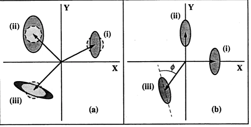
Figure 2.2: Phasor diagrams comparing squeezed states and various other states. (a) Squeezed states by definition are non-classical. The probability distribution along some axis must be narrower than that of the corresponding coherent state. This is clearly true is cases (i) and (iii), although the latter is not a minimum uncertainty state. (Other states have been added for comparison.) However, state (ii) although still represented by an ellipse, is purely classical because the ellipse is always broader than the circle of the coherent state. It could be regarded as “classical squeezing” in some sense.
(b) Various types of squeezing are shown here, (i) is a quadrature amplitude squeezed state, (ii) is a quadrature phase squeezed state and (iii) is a quadrature squeezed state which falls neither into the category of amplitude or phase.
2 .3 .4
Squeezed sta tes
The idea of squeezed states was introduced in the last section, a state for which the standard errors in the two quadratures are different. An example of a squeezed state is given at (i) in Fig. 2.2a. In particular, for a state to be referred to as squeezed, one of these standard errors must be less than one. Even though a state where this is untrue, (ii), may still be considered “squeezed” in a classical sense by the fact that its distribution leads to an ellipse on the quadrature diagram, the term squeezing is usually reserved for the former, because it is non-classical, something which cannot be described without the concepts of quantum mechanics. States (ii) and (iii) are not minimum uncertainty states. However, unlike (ii), (iii) is non-classical and thus squeezed, as its ellipse is narrower than the circle of the coherent state.
[image:34.559.76.510.64.284.2]C H A P T E R 2. THEORY; B A C K G R O U N D , DEFINITIONS A N D TOOLS 23
the quadrature diagram can be at an arbitrary angle to the complex amplitude vec
tor of the state. This means that the squeezing may not be in either the amplitude
or the phase quadratures. In addition, it can also be at an angle <f> to the reed axis
of the phasor diagram. Thus squeezing may not be aptly described by the variables
X a and Ya as they have been defined in the previous section. We need to produce a
more general squeezed state representation, with the quadratures X'a and Ya'. This
is done below.
The unitary squeeze operator is defined as
S ( a ) = exp(-cr*a2 — - vgl*2) where
z z
a = r e 2i4>
The properties of the squeeze operator are
5 t(cr) = S ~1(a) = S ( —a)
S\ ( r) aS( (r ) = a cosh(r) — a^e-2*^ sinh(r)
5 +(<r)at5(ör) = a* cosh(r) — ae2x<t> sinh(r)
S V ) ( * : + iY^S(<r) = X'ae~r + i Y y where
X'a + iY; = ( X . + » y .) e - * (2.21)
We create the squeezed state from the vacuum state in the following manner.
I a, a) = D(a)S(cr) |0) (2.22)
The standard errors in the new quadratures are
SX'a = e~r
6Y' = er (2.23)
These are the minor and major radii of the ellipse in the complex plane, d and
D respectively. Note that the area of the ellipse * d D — ?re~r er = x is independent
of the amount of squeezing.
What does the annihilation operator a do to a squeezed state?
a \ a , a ) = aZ>(a)5(cr)|0)
5 t(or)Z)t(a )a |a ,(r) = { S \ a ) a S ( a ) + 5 t(<r)a5(<r))|0)
CHAPTER 2. THEORY; BACKGROUND, DEFINITIONS AND TOOLS 24
Figure 2.3: Transition from coherent state to number state.
The coherent state is one of m i n i m u m uncertainty, and has equal uncertainty in both its
quadrature amplitudes. A number or Fock state on the other hand, while still a minimum uncertainty state, has a completely random phase, and definite photon number. On the phasor diagram, a Fock state is an annulus of radius y/n and width 1/(2y/n). Some possible intermediate or “banana” states are also shown here.
Thus
a|a,<r) = a|a,<r) — e 2i* sinh(r)D (a)5(<r)|l) (2.24) Thus the squeezed states are not exact Eigenstates of the annihilation operator, nor are their Eigenvalues exactly the amplitude of the original coherent state, but they are close provided that a r. This is important, as it could give a hint for why the linearisation models used later could break down for very large squeezing.
From this it is easy to see that the average number of photons in a squeezed mode is
n = (TV) = |a |2 -I- sinh*(r) (2.25) This is slightly more than a coherent state of the same amplitude. This is not very surprising, but note that it also applies to the vacuum state. A squeeze operator applied alone to a vacuum state gives an average occupation number of sinh3(r) ! In other words, the squeezed vacuum is not empty, not a minimum energy state, indeed not a vacuum at all.
CHAPTER 2. THEORY; BACKGROUND, DEFINITIONS AND TOOLS 25 the quadrature squeezed states which we discussed above, in that they appear on the complex plane as an annulus of radius y/n and width 1/(2y/n) (to preserve area) centered on the origin. They have a definite number of photons (n) and a totally random phase. There are a whole range of states that exist between the Fock state In), and the coherent state of average photon number n = n. This transition is shown in Fig. 2.3. For small amounts of squeezing, they approximate amplitude quadrature squeezing.
These states are often discussed using the term “sub-Poissonian”, implying that the photon number distribution is narrower than Poissonian, the latter being that of a coherent state. In order to examine this, let us take the variance of the photon number.
V (n) = ((a*a)2) — (a*a)2 Evaluated over a coherent state |a), this gives
(2.26)
Thus
V (n)a (|a|< + |a|’) - ( M 2)J
n (2.27)
(6n)a = y/n (2.28)
Thus the variance for a coherent state is just the mean photon number, or, the standard error is the square root of the mean photon number.
Let us try this for the Fock state.
F (n )n = (n2 — n + n) - (n)2
= 0 (2.29)
Thus the photon number distribution for the Fock state has no width. For interest, let us examine the photon number variance of the squeezed vacuum state
V{n )(o,<r) = ti(1 + cosh(2r))
CHAPTER 2. THEORY; BACKGROUND, DEFINITIONS AND TOOLS 26 Hence we can see that the photon statistics for a squeezed vacuum state are always super-Poissonian.4
A useful way of looking at the variance of a field is via the fano factor
V(n) n
It is useful because it is a measure of the type of state which is independent of its intensity.
/ = 0 for a Fock state
/ < 1 for a sub-Poissonian state / = 1 for a coherent state
/ > 1 for a super-Poissonian state
Note that the fano factor is undefined for a vacuum state, but interestingly, it is defined and greater than 1 for a squeezed vacuum.
2.3.5
In ten sity squeezing vs quadrature squeezing
The terms “number” or “intensity” squeezing are used to represent the squeezing process which eventually turns a coherent state into a Fock state, ie bends the circle into a banana which eventually joins up on the opposite side of the phase diagram to become an annulus as shown in Fig. 2.3, and discussed in section 2.3.4. It is this kind of state to which the term “sub-Poissonian” is applied, and fano factors and photon number variances as defined earlier are used.
Amplitude quadrature squeezing means deforming the circle into an ellipse with the minor axis coincident with the amplitude vector. This is also called “in- phase quadrature squeezing”, ie the fluctuations in-phase with electromagnetic field are being reduced, and those out-of-phase, or “in-quadrature”, are being increased. Phase quadrature squeezing means deforming the circle in the opposite manner to the above, and is thus “out-of-phase squeezing”. These two types of squeezing were shown in Fig. 2.2b, in section 2.3.4. In this thesis, these are referred to respectively as “quadrature amplitude” and “quadrature phase” squeezing. Note that any other orientation of the ellipse is possible, such as occurs in Kerr states mentioned in chapter 1.
Despite the different terminology, for small amounts of squeezing, intensity
CHAPTER 2. THEORY; BACKGROUND, DEFINITIONS AND TOOLS 27 and amplitude squeezing are approximately the same thing. The reduced amplitude quadrature variance gives rise to lower photon number variance and thus a sub- Poissonian field. However, for large amounts of amplitude quadrature squeezing, the intensity again becomes noisy, even super-Poissonian. Conversely, as number squeezing progresses, it is clear that the amplitude quadrature variance first de creases, but then increases again, to the final point of becoming a Fock state, perfect number squeezing, having extremely large variances in both quadratures, 2n + 1.
2.3.6
R ep resen tation o f m od es, and linearisation
Before we can treat a real cavity in the laboratory and derive spectra and squeezing behaviour, we need a few more tools.
It is normal to use the annihilation operator a to represent a cavity mode. Examining Eqn. (2.1) we see that it is proportional to the electromagnetic field. Also, in section 2.3.2 when we applied the annihilation operator to coherent states, we found that they were Eigenstates, giving the complex amplitude a as the Eigenvalue. Looking at this, it makes perfect sense for such a representation, although we soon forget the term “annihilation operator a” and just think of it as “mode a”.
The equation of motion or Langevin equation for a cavity mode will be a first order differential equation, describing the rate of change of this mode. See Eqn. (2.34) as an example. While it is not obvious what the rate of change of an annihilation operator really means, it suffices to know that the expectation value of this operator appearing in this equation gives the (generally complex) average field amplitude of the mode concerned.
We can now understand why linearising such an operator makes sense. The cavity mode is linearised by writing the annihilation operator as a sum of the co herent amplitude of the state, or its semi-classical value, and a small fluctuation operator thus,
a = a + 6a (2.31)
CHAPTER 2. THEORY; BACKGROUND, DEFINITIONS AND TOOLS 28
6Xa = 8a + 8a*
8Xxin — 8 Ain + 8A\n
i8Ya = 8a — 8a^
iSYjun = 8 A in - 8 A l
etc (2.32)
giving the fluctuations of the amplitude and phase quadratures in time. Fourier transforming these gives the equivalent fluctuations in frequency space, and then the noise spectra are readily found.
2.3.7 Taking the Fourier transform
When the Fourier transform of an equation is taken, the time dependent quantities, for example 6X = £X(t), will be replaced with their Fourier transforms, denoted by a “tilde” and defined thus
6X = 6X{v) =
*•(«(*))
f O O
= / SX(t) e"“‘dt (2.33)
J—oo
The Fourier transform obeys the normal rules for derivatives and convolution.
■F(/(O®0(O) =
K“)9(u)
2.3.8 Deriving spectra
In this thesis, the spectrum of the time dependent fluctuations of a quantity is found in the following manner. As an example, consider the following differential equation for time dependent amplitude fluctuations.
8X = —a8X + b8X'
CHAPTER 2. THEORY; BACKGROUND, DEFINITIONS AND TOOLS 29
-iu>6X = - a S X + bSX'
SX bSX' a — no
The noise power spectrum can be found from by taking the self correlations
V = (SXySX1)
b*(SX
a2 - f a ; 2
b2V' a2 + a;2
It is assumed here that X' is an input field amplitude (or phase) quadrature operator, and thus its self correlation yields the amplitude (or phase) spectrum of
the corresponding input field. Thus for input (and output) fields we write
{6Xj t SXl) = ^
If however, X' is a complex function of other operators, then its self correlation yields the absolute square of this function, which itself would contain the spectra of
these operators. If on the other hand, X' is the vacuum field, then V = 1.
It is assumed that different field fluctuations are independent, or else they
could have been expanded in terms of independent fields. The cross terms between
independent fields are zero.
(SXi,SXl) = 0 , j ± k
Although only a trivial example, it shows that the output spectrum of a device
is a function of the input spectra, whether they be derived from a laser system or
just the vacuum, and the dynamics of the device. For more rigorous definitions of
spectra see reference [42].
2.4
S im p le C a v ity S y ste m s
2.4.1
T he equations o f m otion, input and output
In section 2.3.6 we discussed the basic idea of an equation of motion for a cavity
CHAPTER 2. THEORY; BACKGROUND, DEFINITIONS AND TOOLS 30 know how to find the fluctuations of the cavity mode in time and frequency space, and find a spectrum. However, no one ever “sees” a cavity mode, or detects it.5 6 To continue, we must know how to couple in and out of the cavity.
We begin again with the equation of motion. This is a rate equation, describ ing the damping of the cavity mode and the input to this mode from the external environment. In order to describe these effects, whether the rate equations be semi- classical or fully quantum in nature, we require the various coupling or loss rates to the inputs and outputs of the external environment. Let us choose a simple single ended cavity equation as an example. A single ended cavity is one with a perfect mirror and a coupling mirror. Let this particular single ended cavity have no loss mechanisms other than the coupling mirror. Its equation of motion is
ä = —na + \/2k Ain (2.34)
Here a is the cavity mode annihilation operator and A{n is the field incident on the coupling mirror. The coupling constant for the mirror, and thus the whole cavity in this case, to the environment, is k.
There are a number of questions which could concern the uninitiated at this stage. Firstly, what is ac, secondly, if a is the annihilation operator of the cavity mode
and A ^ is the amplitude of the incident field, how are they related, and thirdly, why are the constants preceding a and Ain different?
We begin with k. It is inserted into the equation of motion as the linear
decay constant of the amplitude. Thus in time, in the absence of input fields, the amplitude would go like e ~ Kt where t is the time in seconds. Hence k has the units of angular frequency. We can gain even more insight by reconsidering the equation in terms of photon number. Using Eqn. (2.34) and its conjugate equation, we find that
N = a^ä + ä^a
= —2kN + V2k (a*Ajn 4- A\na) (2.35) Assuming a coherent state or a squeezed state (provided a r), taking the expectation value of the above gives an equation in average photon number
n = — 2/cn + \/2/c (a*A;n + A?na) (2.36)
CHAPTER 2. THEORY; BACKGROUND, DEFINITIONS AND TOOLS 31 Thus the decay rate of the photon number in the cavity is 2k. Hence 2k is the coupling rate in photons per second out of the cavity.
Since the number of photons in the cavity is proportional to the energy in the cavity, 2k is the energy coupling rate, and we can write that in the absence of input
fields, the energy goes as
S = Eoe~2Kt (2.37)
In addition, 2k is also the natural linewidth of the cavity system, in angular
units. This is seen by comparing the denominators of equations such as Eqns. (5.17) and (5.18) in section 5.2.2 to that of a standard Lorentzian profile. [47]
This brings us to the second question, what is the relationship between the external fields and the cavity mode? Examining Eqn. (2.34), we see that since a
is unitless (it is a quantised complex number), Ain must have units of s~1^2. It seems odd that they are different at first. However, there is something about the mode a which we haven’t considered yet. Since its expectation value is the complex amplitude a, and since |a |2 is the mean photon number, then this value must change with the size of the cavity; a bigger cavity, can hold more photons for the same input field. Thus, the relationship between a and Ain must change as the cavity size changes. This occurs through the different powers of k preceding the operators.
(We shall see in section 2.4.2 that k is a function of the cavity length.)
In actual fact, A{n is what is termed an “input operator”. It is the Fourier transform of the annihilation operator for a multi-mode external field. [48] Note that
A\nAin has units of s~l . It is thus useful to view this quantity as the intensity of the input field in photons per second. Hence the constant in front of Ajn, is the square root of the photon per second coupling rate, 2k.
Another question; in Eqn. (2.35), why is the input term in the form that it is, rather than A]nAin1 The reason is, that the latter doesn’t allow for interference between the input field and the cavity mode, where as the former does.
The cavity mode is coupled to the output field in a similar way to that which the input field is to the cavity mode, except that the fields which are already present outside the cavity system must be accounted for. Even if there is no average field incident on an output coupling mirror, the vacuum fluctuations incident on it must still be considered. For the simple cavity above, this output equation, or boundary condition is
CHAPTER 2. THEORY; BACKGROUND, DEFINITIONS AND TOOLS 32 where Arefi is the reflected field, and r is the amplitude reflection coefficient of the front mirror. Since r is the square root of the reflectance R, it is normally close to unity for even only moderately good cavities. For example, for the mode cleaner, Rin = 0.98, so r\n = 0.99. Thus for us it is a good approximation to assume that r = 1. It is also desirable, because it allows us to write equations only in terms of input/output operators, modes, and loss rates in photons per second. Hence we rewrite the above equation as
Arefi = CL — Ain (2.39) If we pre-multiply Eqn. (2.39) by its conjugate equation we get
A l*fiA refi = 2/cata + A\nA in - V 2k (aj A in + A]na)
Taking the expectation value as before,
\Ärefi\2 = 2/cn + |Ä^n|2 - c (a*Äin + Ä*na) (2.40) we see that the reflected intensity in photons per second consists of the leakage from the cavity in photons per second times the mean number of cavity photons, plus the reflected input field intensity in photons per second, but then, minus the interference terms, which is where all the interesting physics is.
Having explained what the coupling rates in the equations of motion mean and how the cavity mode is coupled to the external fields, it now remains to relate them to real parameters that are used in designing and building optical cavity systems in the laboratory. These two things provide valuable insight into the physics of cavity systems for the experimentalist.