This is a repository copy of
Alternative method for predictive functional control to handle
an integrating process
.
White Rose Research Online URL for this paper:
http://eprints.whiterose.ac.uk/133014/
Version: Accepted Version
Proceedings Paper:
Abdullah, M. and Rossiter, J.A. orcid.org/0000-0002-1336-0633 (2018) Alternative method
for predictive functional control to handle an integrating process. In: Proceedings of 2018
UKACC 12th International Conference on Control (CONTROL). Control 2018: The 12th
International UKACC Conference on Control, 05-07 Sep 2018, Sheffield, UK. IEEE , pp.
26-31. ISBN 978-1-5386-2864-5
https://doi.org/10.1109/CONTROL.2018.8516787
© IEEE 2018. Personal use of this material is permitted. Permission from IEEE must be
obtained for all other users, including reprinting/ republishing this material for advertising or
promotional purposes, creating new collective works for resale or redistribution to servers
or lists, or reuse of any copyrighted components of this work in other works. Reproduced
in accordance with the publisher's self-archiving policy.
[email protected] https://eprints.whiterose.ac.uk/ Reuse
Items deposited in White Rose Research Online are protected by copyright, with all rights reserved unless indicated otherwise. They may be downloaded and/or printed for private study, or other acts as permitted by national copyright laws. The publisher or other rights holders may allow further reproduction and re-use of the full text version. This is indicated by the licence information on the White Rose Research Online record for the item.
Takedown
If you consider content in White Rose Research Online to be in breach of UK law, please notify us by
Alternative Method for Predictive Functional
Control to Handle an Integrating Process
Muhammad Abdullah
∗and John Anthony Rossiter
† ∗†Department of Automatic Control and System Engineering,University of Sheffield, Mappin Street, S1 3JD, UK.
Email: [email protected]∗ and [email protected]†
∗Department of Mechanical Engineering,
International Islamic University Malaysia, Jalan Gombak, 53100, Kuala Lumpur Malaysia. Email: mohd [email protected]∗
Abstract—This work proposes an improved method for Predic-tive Functional Control (PFC) to handle an integrating process. Instead of assuming a constant future input, the dynamic is shaped with a first-order Laguerre polynomial so that it converges to the expected steady state value. This modification provides simpler coding and tuning compared to the conven-tional method in the literature. Simulation results show that the proposed controller improves the consistency of the open-loop prediction of an integrating process and thus improves closed-loop performance and constraint handling properties. The practicality of this algorithm is also validated on laboratory hardware.
Index Terms—Predictive Control, PFC, Laguerre Function, Constraints, Integrating Process, Transparent Control, Servo System.
I. INTRODUCTION
Predictive Functional Control (PFC) is a simple version of Model Predictive Control (MPC) developed in the early 1970s [1]. This algorithm only requires simple coding and low-level computation while retaining similar benefits to MPC in handling constraints and/or delays [2]. Despite its appealing characteristics, PFC receives relatively little interest in the literature [3] as it does not easily have rigorous properties such as stability assurances [4], [5] or robust feasibility [6]. However, the key selling point of PFC is the simplicity in tuning and implementation; it is a competitor to PID rather than the conventional predictive controller.
The simplistic PFC concept has several limitations, espe-cially when dealing with an integrating process [2]. Due to their marginally stable dynamics, the constant future input assumption of PFC gives a divergent open-loop prediction [2], [7], [8]. Consequently, it may lead to poor closed-loop performance, prediction inconsistency, and also a failure in constraint implementation. Nevertheless, for low-level control applications where PID is unable to handle a constraint, PFC is still considered as an attractive option. Thus, the aim of this paper is to overcome some weaknesses while maintaining the formulation simplicity and cost effectiveness of PFC.
To deal with open-loop unstable plant, PFC practitioners often employ a cascade like structure known as transparent
This work is funded by International Islamic University Malaysia and Ministry of Higher Education Malaysia.
control [2]. The inner loop consists of a proportional controller to stabilise the system predictions, and PFC provides the target trajectory via an outer loop. In practice, this structure often works better than PID within a constrained environment. However, the use of constant future input assumption can still lead to ill-posed decision making which impacts on both closed-loop performance [9] and constraint handling [10]. The interaction between inner and outer loops also makes the tuning and constraint implementation less transparent and, within the literature, there is no clear or systematic explanation of the approach.
Recent work has shown Laguerre PFC (LPFC) can im-prove closed-loop performance, prediction consistency and constraint handling for a stable system [9], [10]. This paper explores its capability to handle an integrating process. LPFC shapes the future input trajectory to converge to steady state with 1st order dynamics; this framework can stabilise the open-loop prediction of an integrating system without requiring a cascade structure, thus retaining a standard, and simpler, PFC formulation. Moreover, the Laguerre pole can be used to fine tune the closed loop performance [9], [11] and facilitate more reliable constraint management. The required modification is straightforward and thus in line with the simplicity require-ment.
Section II gives some background on the nominal PFC and LPFC frameworks. Section III introduces the transparent control and LPFC law to handle an integrating process. Sec-tion IV provides a numerical example and analysis for both approaches. Section V validates the results with laboratory equipment simulations and section VI provides conclusions.
II. PFC FORMULATION FORNOMINALSYSTEM
A. Traditional PFC
A PFC framework is based on simple human concepts and computes a required control action depending on how fast a user expects/desires the output to reach the target. There are two main components in the PFC formulation which are the desired target trajectory and system prediction. The control law is calculated by enforcing the following equality:
yk+n|k =R−(R−yk)λn (1)
whereyk+n|k is the n-step ahead system prediction at sample
time k. The right hand side of (1) represents the desired trajectory of the output from yk to the target value R with
a convergence rateλ. The two main tuning parameters are:
• The coincidence horizon n defines the point where the system prediction matches the target trajectory.
• The desired closed-loop pole λ = e−3T /CLT R, with T the sampling time and CLT R the closed-loop time response.
Since the n-step ahead prediction algebra of a linear transfer function mathematical model is well known in the literature (e.g. [12]), here only the key results are provided. For inputs uk and outputsyk, the n-step ahead linear model prediction is
given as:
yk+n|k=Hnu→k+Pnu←k+Qnyk
← (2)
where parametersHn,Pn,Qn depend on the model
parame-ters and for a model of orderm:
u→k =
uk uk+1
.. . uk+n−1
;u←k=
uk−1
uk−2
.. . uk−m
;yk
← = yk yk−1
.. . yk−m
(3) The control input is computed by substituting the prediction (2) directly into (1) to obtain:
Hnuk
→+Pnu←k+Qny←k =R−(R−yk)λ n
(4)
Adding a constant future input prediction assumptionuk+i|k = uk, i= 0, ..., nand defininghn =P(Hn), the nominal PFC
control law reduces to:
uk
→ =
R−(R−yk)λn−(Pnu←k+Qnyk ←) hn
(5)
Remark 1:The tuning parameterλshould make the design process transparent, however the selection of coincidence horizonnaffects the efficacy of λdue to the constant future input assumption [7]. With small horizons, the effectiveness of λis more significant, but there may be poor prediction consis-tency with the target behaviour resulting in poor closed-loop behaviour. Conversely, larger horizons gives better prediction consistency but reducing the effectiveness of λ as a tuning parameter.
Remark 2:Prediction consistency is important for effective constraint handling thus, for some challenging dynamics, a constant input assumption may be ineffective [10].
B. Laguerre PFC (LPFC)
The LPFC approach utilises the expected constant steady-state input uss to eliminate the offset. The z-transform of
discrete Laguerre polynomials are [11]:
L(z) =p1−a2(z
−1
−a)j−1
(1−az−1)j ; 0< a <1 (6)
wherejis the order of Laguerre function andais the Laguerre pole which depends on a user selection between 0< a < 1. For simplicity of coding and concept, a first-order Laguerre polynomial is employed here, although high order polynomials may be used [11], [13], [14]. The function with altered scaling becomes an exponential decay as:
L(z) = 1
1−az−1 ≡ 1 +az
−1
+a2
z−2
+· · · (7)
Hence, the future input prediction is parametrised as:
uk+n=uss+Lnη; Ln=an; L= [1, a,· · · , an−1] (8)
where η is a degree of freedom. The parametrisation of (8) gives output predictions which converge to the steady-state exponentially with a ratea. Thenstep ahead output prediction is derived by substituting (8) into (2):
yk+n|k =hnuss+HnLnηk+Pnuk
←+Qny←k (9)
Hence, the LPFC control law is defined by substituting prediction (9) into (1) and solving for parameter η as:
ηk =
R−(R−yk)λn−(Pnuk
← +Qny←k)−hnyuss
HnLn
(10)
Due to the receding horizon principle [11] and the definition of L(z)in (7), the current inputuk is:
uk=uss+ηk (11)
Remark 3:By shaping the future input dynamics, LPFC can improve prediction consistency, closed-loop performance and the efficacy ofλas a tuning parameter [9]. This improvement also provides a more accurate and less conservative solution when satisfying output/state limits [10].
III. PFC FORMULATION FORINTEGRATINGSYSTEM
A. Transparent Control
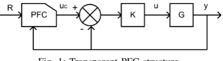
[image:4.595.59.277.149.209.2]Transparent control utilises two level of cascade structure (see Fig. 1). The inner loop employs a proportional gain with negative feedback to stabilise the open loop prediction, while nominal PFC controls the outer loop and eliminates any offset due to disturbance and enhances the overall dynamic performance [2].
Fig. 1: Transparent PFC structure.
The inner loop with gain K will be used as a prediction model as in (12) instead of the plant modelGto compute the manipulated inputuc.
y(s) = GK
1 +GKuc(s) (12) The actual inpututhat will be send to the plant is:
uk =K(uc,k−yk) (13)
With this technique, the controlled system is able to maintain regulation during set-point changes by introducing a temporary over-compensated set-point [2]. At the same time, the outer loop will minimise the tracking error using a standard PFC formulation as discussed in section II-A.
Remark 4: Transparent PFC (TPFC) only accepts propor-tional gain rather than the combination with integral and/or derivative to keep the constraint implementation purely al-gebraic [2]. To implement input or rate constraints, a back calculation procedure is needed to transfer the information from the inner loop to the outer loop and avoiding saturation as:
yk+ umin
K ≤uc,k≤yk+
umax
K (14)
yk+
∆umin+uk−1
K ≤uc,k≤yk+
∆umax+uk−1
K (15)
Since the constraint is implemented at the current time only, there is no check that the implied predictions satisfy con-straints in the future and thus recursive infeasibility may result.
Remark 5: For output or state constraints, the traditional practise utilises a multiple PFC regulators that run in parallel [2], [10]. The first regulator computes the preferred control action while the second regulator produces an input to satisfy the limit. A supervisor will choose the correct input for the plant. However, advances in computation technology mean this tedious ad hoc approach can be replaced with a more systematic, but simple, approach such as in [15].
B. Laguerre PFC for Integrating Process
Due to the pole on the origin, the steady state input for an integrating process is zero for a constant set point. These dynamics are still compatible with a LPFC law (section II-B) with the only required modification being to defineuss = 0.
Theorem 1: The future input dynamics of u(z) = uss
1−z−1 +
ηk
1−az−1 (16)
will give input predictions that settle exponentially at zero with a speed linked to Laguerre polea. For an integrating process, the value ηk effects the implied steady-state outputs.
Proof: The signal defined in (16) has the property that
lim
k→∞uk =uss ⇒ klim→∞yk=R (17)
Whenuss= 0, the steady-state output has affine dependence
on the integral of the future input.
Remark 6: For simple first order system the value of a should be equal to λ[9]. However for a higher order system, selecting a < λ will give faster convergence to steady state and thus can improve the prediction consistency.
Algorithm 1 (LPFC): For integrating process, a similar algorithm as in (10) is used except that uss term is removed.
ηk =
R−(R−yk)λn−(Pnuk
←+Qny←k) HnLn
(18)
Theorem 2: Using LPFC input predictions as defined in
Algorithm 1, output, state and input constraints can be rep-resented by a set of linear inequalities.
Proof: Output constraints can be constructed from the
output predictions in (9) within the validation horizonni and
comparison with the limits at each sample instant, e.g.:
ymin≤HniLniηk+Pniu←k+Qniy←k ≤ymax, ∀i >0 (19)
The maximum/minimum input rate/value occur at the first sample, so input constraints can be formulated as:
umin≤ηk≤umax (20)
∆umin≤ηk−uk−1≤umax (21)
Combining (19,20,21) it is clear that for suitableM, vkone can
represent the satisfaction of constraints by predictions using a single vector inequality of the form:
M ηk ≤vk (22)
We can now define the constraint handling algorithm which is akin to methods given in [15].
Algorithm 2: [LPFC constrained] Use the unconstrained law (18) to determine the ideal value of ηk and check each
constraint in (22) using a simple loop (subscripts denote position in a vector).
Set umax=∞, umin=−∞.
For i=1:end,
ifMiηk 6≤vi &Mi>0 then defineumax=vi/Mi,
ifMiηk 6≤vi &Mi<0 then defineumin=vi/Mi,
end loop.
if ηk < umin,ηk=umin. if umax< ηk,ηk =umax.
Define u(k)using (16).
Remark 7: Infeasibility can arise due to too fast or large changes in the target. However, LPFC helps in this case because the exponential structure embedded into the input prediction automatically slows down any over aggressive input responses and thus significantly increases the likelihood of feasibility being retained. In the worst case, set point changes need to be moderated as in reference governor approaches [16].
The summary benefits of this algorithm are:
• It offers a simple and systematic framework to handle an integrating process.
• It stabilises the output prediction without a cascade structure thus no back calculation process (Remark 4) is needed for input/rate constraints.
• The Laguerre poleacan be utilised to control the speed of convergence to improve the prediction consistency and efficacy of constrained solution.
• The implied structure of (16) in conjunction with con-straints (22) means that a recursive feasibility guarantee (nominal case) is provided [15].
IV. NUMERICALEXAMPLES ANDANALYSIS
This section presents a numerical example to demonstrate the benefit of using LPFC compared to TPFC. A first order servo system with integrator is considered as a plant where the control objective is to track the position. The discrete mathematical model with sampling time 0.02s is:
G= 0.0095z
−2+ 0.0073z−1
1−1.45z−1+ 0.45z−2 (23)
This simulation will focus on the tuning process and the concept of well-posed decision making that can be observed by comparing the open-loop prediction and closed-loop behaviour of the controller. In addition, the efficacy of constraint handling is also discussed in the last subsection.
A. Tuning and Performance of TPFC
The first step in implementing TPFC is to tune the pro-portional gain before selecting the coincidence horizon n. This gain K will determine the convergence speed and the steady state error of the inner-loop. Small gain leads to slower responses, while too large a gain causes oscillatory behaviour. The root-locus (continuous time) plot shows that the choice K = 6.45 is around a critical value in that higher K would give oscillatory poles (see Fig. 2).
The coincidence horizon is selected by comparing the step response with a desired first order target trajectoryrwithλ= 0.74 (refer to Fig. 2). Since the inner loop is second order (due to the added integrator), it is necessary [7] to choose a coincidence horizon in the range3≤n≤8; lower values are often preferable so heren= 3.
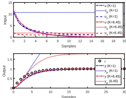
Fig. 3 shows the closed-loop and predicted (at sample k= 0) performance of TPFC with different values of gainK. The actual closed-loop behaviour is expressed as y (output) and u (input), while the implied predictions are denoted by signals output yp and input up (corresponding to first value
-40 -30 -20 -10 0
-20 0 20
K=3 K=6.45
Root Locus
Real Axis (seconds-1)
Imaginary Axis (seconds
-1)
0 2 4 6 8 10 12 14 16 18 20
Samples 0
0.5 1
Output K=3
[image:5.595.321.526.57.224.2]K=6.45 r
Fig. 2: Root locus and step response of 1+GKGK with different gainK.
0 2 4 6 8 10 12 14 16 18 20
Samples
0 5 10 15
Intput
u (K=1) up (K=1) uc (K=1) u (K=6.45) up (K=6.45)
uc (K=6.45)
0 5 10 15 20 25 30
Samples
0 0.5 1 1.5
Output
r y (K=1) yp (K=1) y (K=6.45) yp (6.45)
Fig. 3: Closed-loop and open-loop behaviour of Gfor TPFC with different K.
of input produced by PFC uc instead of the actual inputu) .
For both choices of K, in the unconstrained case, the closed-loop outputsy track the trajectory set pointrand with almost equivalent speed. However, withK= 1, the implied prediction yp has a very slow convergence in response to the constant
input dynamics up and is inconsistent with the closed-loop
behaviourythat results. With a higher gain value (K= 6.45), the consistency is improved but still poor. This inconsistency is likely to lead to severely flawed decision making should constraint handling be required.
B. Improvement on Prediction Consistency with LPFC.
For LPFC, due to the presence of an integrator, the coinci-dence horizon is selected based on the the impulse response (see Fig. 4) using the guidance of [7]; this suggests a value in the region of n= 3.
[image:5.595.320.527.281.442.2]0 2 4 6 8 10 12 14 16 18 20 Samples
0 0.01 0.02 0.03 0.04
[image:6.595.64.267.53.141.2]G r
Fig. 4: Impulse response of Gwith target trajectoryr
0 2 4 6 8 10 12 14 16 18 20
Samples 0
5 10 15
Intput
u (a= )
up (a= )
u (a=0.56)
up (a=0.56)
0 5 10 15 20 25 30
Samples 0
0.5 1 1.5
Output
y (a= )
yp (a= )
y (a=0.56)
yp (a=0.56)
r
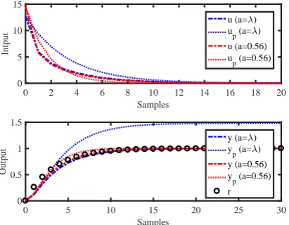
Fig. 5: Closed-loop and open-loop behaviour of Gfor LPFC with varying Laguerre polea.
However, for a higher order system, this value needs to be further tuned as it has an impact on the convergence rate of the output prediction when tracking the first order target trajectory (Theorem 1). Fig. 5 shows that with a choice of a=λ, while the controller still tracks the set point well, there is still noticeable inconsistency between predictions yp and
the closed-loop behaviour y. However, reducing the pole to a= 0.55improves the prediction consistency and the overall closed-loop performance is still good (Remark 6).
C. Improvement in Constrained Performance with LPFC
One of the key selling points of PFC is the computationally simple (low cost) constraint handling ability. When the system input is bounded to umax = 8 (see Fig. 6), both of the
controllers manage to track the set point and satisfy the given limit although LPFC gives a slightly better closed-loop performance due to the well posed decision. Moreover, the LPFC formulation is more straightforward to implement and does not require back calculation methods (Remark 4).
Fig. 7 shows the system response of both controllers when the output is limited toymax= 0.8. The validation horizon is
selected atni = 10to cover most of the transient period and
prevent constraint violation at the early stage. In this case the closed-loop response of TPFC is slower and more conservative in satisfying the limit due to the prediction inconsistency demonstrated in Fig 3. Conversely, LPFC which is based on more consistent predictions (see Fig 5) converges much faster
0 2 4 6 8 10 12 14 16 18 20
Samples 0
5 10
Intput
u (TPFC) u (LPFC)
0 5 10 15 20 25 30
Samples 0
0.5 1
Output y (TPFC)y (LPFC)
[image:6.595.321.525.59.219.2]r
Fig. 6: Closed-loop response of Gfor LPFC and TPFC with bounded input (umax= 8).
0 2 4 6 8 10 12 14 16 18 20
Samples 0
5 10 15
Intput
u (TPFC) u (LPFC)
0 5 10 15 20 25 30
Samples 0
0.5 1
Output y (TPFC)y (LPFC)
r
Fig. 7: Closed-loop response of Gfor LPFC and TPFC with bounded output (ymax= 0.8).
compared to TPFC. Clearly the constrained solution of LPFC is more accurate and less conservative.
V. IMPLEMENTATION ONREALHARDWARE
To validate the practicality of LPFC, the algorithm is tested on a Quanser SRV02 servo based unit powered by a Quanser VoltPAQ-X1 amplifier (see Fig. 8). This system is operated by National Instrument ELVIS II+ multifunctional data acquisition. The plant is connected to a computer via a USB connection using NI LabVIEW software. The control objective is to track the servo positionθ(t)by manipulating the supplied voltageu(t). The mathematical model of this system is given as (for more details, refer to [17] user manual):
0.0254¨θ(t) = 1.53u(t)−θ˙(t) (24)
[image:6.595.61.267.183.343.2] [image:6.595.319.528.275.439.2]Fig. 8: Quanser SRV02 servo based unit.
0 1 2 3 4
Time (s)
-1 -0.5 0 0.5 1
Angular speed (rad/s)
y(unconstrained) y(constrained) Target
0 1 2 3 4
Time (s)
-30 -20 -10 0 10 20 30
Voltage (V) u(unconstrained)
u(constrained)
Fig. 9: Unconstrained and constrained performances of LPFC in tracking the Quanser SRV02 servo position.
The algorithm is employed with similar tuning parameters as in the previous numerical example (λ = 0.74, n = 3 and a = 0.55). Fig. 9 demonstrates the unconstrained and constrained performances of LPFC to track an alternating set point between -1 rad/s to 1 rad/s. For the unconstrained case, a similar performance to the simulation studies are obtained. The controller manages to provide a smooth tracking to the desired target while retaining the intuitive link between the target dynamic λ and the closed-loop convergences speed (CLTR = 0.2s). In the constrained case, the implied input limits (−8v≤uk≤8v) and output limits (−0.8≤yk ≤0.8)
are satisfied without any conflict by employing the systematic constraint method (Algorithm 2).
VI. CONCLUSIONS
This work proposes an alternative Laguerre PFC approach to control an integrating process. Since the traditional PFC formulation for integrating processes is unable to give a stable open loop prediction, the transparent controlapproach is often used. Although this cascade structure can stabilise the plant using a proportional controller, the decision making process may still be poorly posed, and notably can lead to a highly conservative solution in the presence of constraints. Conversely, by shaping input predictions using a Laguerre
polynomial, the nominal PFC method can be employed with-out a cascade structure. Besides, the improved prediction consistency of LPFC enables the constrained solution to become more accurate and less conservative, thus improving performance. This paper has also demonstrated the efficacy of the proposed LPFC algorithm on laboratory hardware with active constraints. Critically, the proposed algorithm is very simple to code and implement which in line with the core markets for PFC approaches.
Nevertheless, there is a potential weakness with LPFC especially when the independent model structure is used. A small offset error may occur if there is a model mismatch or the real plant is not in fact integrating. Future work aims to look more closely at this issue while providing a formal sensitivity analysis and systematic design of LPFC in handling uncertainty. Another important consideration is to analyse the alternative shaping methods which may be better tailored to deal with higher order and/or challenging dynamical.
ACKNOWLEDGMENT
The first author would like to acknowledge International Islamic University Malaysia and Ministry of Higher Education Malaysia for funding this work.
REFERENCES
[1] J. Richalet, A. Rault, J.L. Testud and J. Papon, Model predictive heuristic control: applications to industrial processes,Automatica, 14(5), 413-428, 1978.
[2] J. Richalet, and D. O’Donovan,Predictive Functional Control: princi-ples and industrial applications. Springer-Verlag, 2009.
[3] R. Haber, R. Bars, and U. Schmitz,Predictive control in process engi-neering:From basics to applications, chapter 11, Wiley-VCH, Germany, 2012.
[4] J. Rossiter, A priori stability results for PFC,IJC, 90(2), 305–313, 2016. [5] P.O. Scokaert and J.B. Rawlings, Constrained linear quadratic regulation,
IEEE Trans. on Automatic Control, 43(8), 1163–1169, 1998.
[6] J. Mayne, M.M. Seron, and S. Rakovic, Robust Model Predictive Control of constrained linear systems with bounded disturbances,Automatica, 41(2), 219–224, 2005.
[7] J. A. Rossiter, and R. Haber, “The effect of coincidence horizon on predictive functional control,”Processes, 3, 1, pp. 25-45, 2015. [8] J. A. Rossiter, “Input shaping for PFC: how and why?,”J. Control and
Decision, pp. 1-14, Sep. 2015.
[9] M. Abdullah and J. A. Rossiter, “Utilising Laguerre function in Pre-dictive Functional Control to ensure prediction consistency,” 11th Int. Conf. on Control, Belfast, UK, 2016.
[10] M. Abdullah, J. A. Rossiter and R. Haber, “Development of constrained Predictive Functional Control using Laguerre function based prediction,” IFAC World Congress, 2017.
[11] L. Wang, Model predictive control system design and implementation using MATLAB®, Springer, 2009.
[12] J. A. Rossiter, Model predictive control: a practical approach, CRC Press, 2003.
[13] M. Abdullah, and M. Idres, Constrained Model Predictive Control of Proton Exchange Membrane Fuel Cell,JMST, 28(9), 3855–3862, 2014. [14] M. Abdullah, and M. Idres, Fuel cell starvation control using Model Predictive Technique with Laguerre and exponential weight functions,
JMST, 28(5), 1995–2002, 2014.
[15] J. Rossiter, B. Kouvaritakis, and M. Cannon, Computationally efficient algorithms for constraint handling with guaranteed stability and near optimality,IJC, 74(17), 1678–1689, 2001.
[16] E. Gilbert and I. Kolmanovsky, Discrete-time reference governors and the non-linear control of systems with state and control constraint,Int. J. Robust and Non-linear Control, 5, 487–504, 1995.
[image:7.595.70.255.228.371.2]