Corner transfer matrices of the Ising model in statistical mechanics

The Ising Model in

St a t i s t i c a l Mechanics

by

Shiu Kuen Tsang ( ^ d> )

A Thesis submitted to

the Australian National University for the degree

of Doctor of Philosophy.

dissertation is an account of my own original work carried out from May,1976 to February,1979 at the Department of Theoretical Physics, Research School of Physical Sciences, Australian National University for the degree of Doctor of Philosophy.

It is my greatest gratitude to thank my supervisor Dr. R. J. Baxter for the supervision, criticism and

encouragement he so willingly gave during the course of the work reported in this thesis.

I am also indebted to Dr. K. Kumar for his advices during Dr. Baxter's brief absence in 1976.

I acknowledge the pleasant atmosphere provided by the staff and colleagues of the Department of Theoretical Physics. In particular, I would like to thank

Prof. K. J. Le Couteur and Dr. I. G. Enting for their stimulating discussions.

A special word of thanks goes to Mr. Stephen K.B. Tin for his care with the typing of the thesis and for his

patience and encouragement over the last three years.

The work of this thesis is mainly on an

investigation of the "corner transfer matrices" (CTM) of the Ising model in statistical mechanics. The thesis starts with a review on the Ising model and is followed by a brief

discussion of various methods for investigating the Ising model. In particular, new techniques and approaches

developed by Baxter form the basis for further research described in this thesis. Thus in Section I, the review is introduced first.

In Section II, the new technique for investigating the zero field, eight-vertex model on the squ are lattice using the CTM suggested by Baxter (1976) is applied to the anisotropic, ferromagnetic, triangular Ising lattice in zero field below its critical temperature. The diagonal form of the CTM of the triangular lattice shows essentially the same structure as that for the square Ising lattice. The spontaneous magnetization can be obtained easily from this method. It is hoped that this technique will give

illuminating insights into the problems of critical phenomena.

convergence of this approach is tested by applying the method to the zero field Ising model on the square lattice. The problem is simplified to that of solving a relatively

small system of non-linear equations. The estimates to the spontaneous magnetization and the critical temperature from the sequence of variational approximations are obtained.

The results converge rapidly to the exact ones. They exhibit a cross-over phenomenon and satisfy a scaling relationship for the spontaneous magnetization. Since this method can be applied to many systems such as the square lattice Ising model with a magnetic field, where the exact solution is not available yet, one may expect to obtain good approximations

to the thermodynamic functions of these models by using this method.

The work described in this thesis has been reported in the following papers :

(i) Tsang, S. K . , (1977) J. Stat. Phys. 17:137-152. 'Corner Transfer Matrices of the

Triangular Ising Model'

(ii) Tsang, S. K . , (1979) J. Stat. Phys. 20:95-114. 'Square Lattice Variational Approximations

Acknowledgment iv

Abstract v

I

1. Phase Transitions and Critical Phenomena 2

2. The Ising Model 7

II

1. Introduction 13

2. The CTM of the Triangular Lattice 16

2.1 The corner transfer matrix 16

2.2 Half-row matrices 20

2.3 Spin matrices 23

2.4 The matrices as a product of spin operators 24

3. The Representatives of the CTM 27

3.1 The spinor representations 27

4.2 The generating function ^(y tz) 37 4.3 Elliptic function parametrization 44

4.4 The contour of integration 47

5. Solution of the Integral Equations 50

5.1 Solution by Fourier transforms 50

5.2 Orthogonality properties of 55

5.3 Analyticity of p ^ ^ (x) 59

6. The Diagonal Form of the Corner Transfer Matrices

and the Spontaneous Magnetization 61

6.1 The diagonal form of the CTM 61

6.2 The spontaneous magnetization 64

Conclusion 65

Appendix IIA The Jacobian Elliptic Functions and

Theta Functions 66

Appendix IIB The Kernel W.(u.,u ) 69

^ J 3o

I I I

TO THE ISING MODEL 77

1. Introduction 78

2. The Variational Approximation 81

2.1 The transfer matrix 81

2.2 The variational approach 84

3. Thermodynamic Properties of the System 94

3.1 Row-column symmetry 94

3.2 Thermodynamic functions 95

3.3 Graphical interpretation of the matrices 99

4. The Sequence of Variational Approximations for

the Isotropic Square Ising Model 105

4.1 Representations in which 4(f) diagonal 105

4.2 Zeroth order approximation 107

4.3 Iterative method of solution 110

4.4 Leading order considerations 112

5. The Variational Equations in Their Representatives 115 5.1 The representatives of the matrices 115

5.2 Iterative method of solution 118

5.3 Symmetry properties of M' 120

5.4 Reduction of the matrix equations 124

6. The Infinite Solution and the Thermodynamic

Functions 132

6.1 The infinite solution 132

6.2 The thermodynamic functions in their

representatives 138

7. The Numerical Method of Solution 142

7.1 Polynomial form of equations 142

7.2 The critical point of the system 148

7.3 The n = 2 solution 149

8.2 The critical temperature 158

8.3 Cross-over phenomenon 162

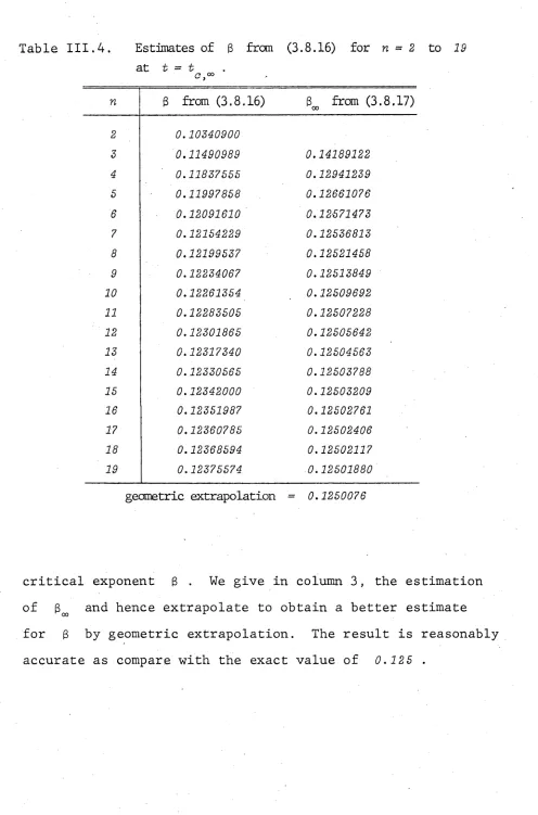
8.4 Estimation of the critical exponent 3 167

Conclusion 169

Appendix IIIA Low Temperature Leading Order Behaviour of the Variational Equations 172 Appendix IIIB Relations between Matrices in their

Representatives 178

FOOTNOTES

Statistical mechanics is the study of the

equilibrium properties of macroscopic systems in terms of their microscopic properties. It was only in 1902 that a comprehensive formulation of statistical mechanics was given by Gibbs (1902). Since then, a better understanding of the relations between the macroscopic description of many physical phenomena through thermodynamics and the underlying atomic theory has been established.

One of the oldest problems in equilibrium

statistical mechanics is the theory of phase transitions. In particular, a great deal of attention has been given to the theoretical and experimental investigation of critical phenomena in phase transitions (Stanley, 1971).

A wide variety of physical systems exhibit

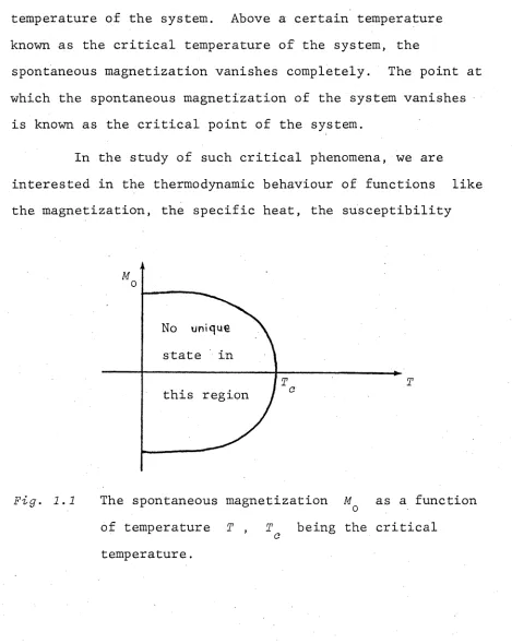
Consider, for example, a system of magnetic spins, in the presence of a strong magnetic field H parallel to the magnetic axis of the system. At sufficiently low

temperature, if we decrease the magnetic field to zero, a spontaneous magnetization of the system remains. Fig. 1.1 shows the change of this spontaneous magnetization with the temperature of the system. Above a certain temperature known as the critical temperature of the system, the

spontaneous magnetization vanishes completely. The point at which the spontaneous magnetization of the system vanishes

is known as the critical point of the system.

In the study of such critical phenomena, we are

interested in the thermodynamic behaviour of functions like the magnetization, the specific heat, the susceptibility

this region

Fig. 1.1 The spontaneous magnetization M as a function of temperature T , T^ being the critical

and the correlation function. Obviously, the spontaneous, magnetization of the system is singular at this point.

It is customary to consider the singularity at the critical point as a power law singularity. That is, we expect that near the critical point, the spontaneous magnetization behaves as

M * ( T - T ) ^ , T + T ~

(

.

.

)

0 v c ' o

where 3 is known as the critical exponent for Mq . Other commonly considered critical exponents are

(i) 6 for the critical isotherm,

H % I M I6 , (1.1.2)

where H is the magnetic field and M the magnetization;

(ii) a j a ' for the specific heat magnetic field,

CH % ( Tc - T .

cH % ( t - t o y a ,

(iii) y , y' for the zero field isothermal susceptibility,

XT ^ ( Tq - T )"Y , T -> T~

(

.

.

)

XT * ( T - Tc )"Y , T - T+o

Cu at constant

tl

T + T

(

.

.

)

(iv) v , v' for the correlation length,

£ v ( T - T )

6 v ( T - T )

s c

-v

-V

T T

T + T

(1.1.5)

(Stanley, 1971).

Consequently, a problem of central interest in the theory of critical phenomena is the determination of the critical exponents governing the approach of the system to the critical point.

Using standard statistical mechanics, for a

molecular system with general intermolecular forces, the relative statistical weight of a state s of the system with y E(s) is given by exp ( - E(s)/kßT ) where k n is the Boltzmann’s constant and T the

D

temperature of the system. By forming the partition function of the system

Z =

I

where the summation is over all allowable states s of the system, we can then derive all the thermodynamic functions of the system by the usual procedures of statistical

mechanics and in particular, one can find out whether the system undergoes a phase transition nv "tkc L'^'t

An ideal model in statistical mechanics should describe the characteristics of a realistic system which is important for the phenomenon under study and at the same time be tractable mathematically. The Ising model provides such a model in the study of ferromagnetism.

The system considered in the model is an array of

N fixed points in a d-dimensional periodic lattice.

Associated with each lattice site j is a spin variable a .

0

which may take up values +1 or -1 . A particular set of values of all the spins constitutes a configuration of the lattice and one may assume particular interactions between spins such as nearest-neighbour or next nearest-neighbour

interactions or even other two-body or many body interactions. However, in general, to resemble the realistic situation, it

is usually assumed that there are only short range forces between the molecules, in particular, that there are only nearest-neighbour interactions.

a model for ferromagnetism. He studied the one-dimensional Ising chain with nearest-neighbour interaction and found no phase transition. There was not much development on the

m o d e l until 1936 w h e n Peierls (1936b) showed that the Ising m o d e l in two and three dimensions did exhibit spontaneous m a g n e t i z a t i o n at sufficiently low temperatures.

Unfortunately, his proof not rigorous and m a s corrected

by Griffiths (1964). In 1941, Kramers and Wannier (1941a,b) investigated, on the square lattice, an Ising model w ith n e a r e s t - n e i g h b o u r interactions only and were able to locate

the transition temperature of the system using a dual transformation relating the low and high temperature

expansions of the p a r t i t i o n function. Appro x i m a t i o n s for the free energy of the system were obtained using a

v a r i a t i o n a l m e t h o d (Kramers and Wannier, 1941b). A major b r e a k t h r o u g h in the development came in 1944 w h e n Onsager (1944), using the transfer m a t r i x formulation of the model (Kramers and Wannier, 1941a; Montroll, 1941), obtained the exact solution of the two-dimensional square Ising model in the absence of a m a g n e t i c field. In 1949, a simplified v e r s i o n of his solution was given by K a u f m a n using spinor algebra (Kaufman, 1949; K a u f m a n and Onsager, 1949).

A l t h o u g h the result for the spontaneous m a g n e t i z a t i o n of the system was announced by Onsager (1949), the derivation was given only in 1952 by Yang (Yang, 1952; Chang, 1952). Exact results for m a n y other lattice systems such as the triangular lattice (Newell, 1950; Wannier, 1950), the

mathematical and physical understanding of the model was provided by Yang and Lee (1952a,b) in their description of the model as a lattice gas and their theorem on the roots of the partition function of the system. In the 1960 s, many different methods for obtaining the exact results were

developed. Examples are the combinatorial method

(Kac and Ward, 1952; Potts and Ward, 1955; Potts, 1955); the Pfaffian approach (Hurst and Green, 1960; Fisher, 1961, 1966; Kasteleyn, 1961,1963; Montroll, Potts and Ward, 1963); the field theory approach (Schultz, Mattis and Lieb, 1964; Hurst, 1966; Gibberd and Hurst, 1967); using perturbation

theory (Herman and Dorfman, 1968) and recently, using

star-triangle relations (Baxter and Enting, 1978; Hilhorst, Schick and van Leeuwen, 1978). However, all these methods merely re-derived the original results: no new results were produced. The two-dimensional Ising model in the

presence of a magnetic field and the three dimensional problem has yet remained unsolved.

It is therefore necessary to investigate these problems using other approximation methods. Some of the better known approximation methods studied are :

(i) Closed form approximation methods including the cluster variation method (Peierls, 1936a; Li, 1949; Kikuchi, 1951; Kikuchi and Brush, 1967); the constant

coupling approximation (Kasteleyn, 1956; Danielian, 1963); and the matrix and variational methods

However, these methods, although they give reasonably good description of the system away from the critical point, fail to account for the correct thermodynamic behaviour of the system near the critical region. Recently, a special approximation method using the variational principle was developed (Baxter, 1978). The method is interesting as it is possible to obtain reasonably good estimates of the critical temperature as well as many other thermodynamic properties of the system with only moderate amount of computational efforts.

(ii) Series expansions in powers of some appropriate variable (Domb, 1949; Sykes, Essam and Gaunt, 1965; Sykes et at,, 1973a,b,c; Domb, 1974). If

sufficient terms in the expansions can be derived, it is possible to estimate the critical temperature and the critical exponents of the system from the

series. In particular, they provide the best

estimates of the critical temperature and critical exponents of the three-dimensional Ising model. However, using the conventional combinatorial technique, enormous amount of computation work is required to obtain the series. Hence, it may be more efficient to obtain the series using algebraic

(iii) Renormalization group method (Kadanoff, 1966; Wilson, 1971a,b). In this method, one focusses

attention on the critical region directly, by means f f o ö t / v ö t e .

of a sequence of transformations. Though very good estimates of the thermodynamic functions of the systems considered may be obtained using simple

approximation methods (Kadanoff, 1975; Southern, 1978) no exact result has yet been arrived through this

approach, with the exception of the recent derivation of the critical exponent a of the two-dimensional Ising model by Hilhorst, Schick and van Leeuwen (1978)

Despite all the intensive studies on the model,

exact results have only been obtained in the two-dimensional case in the absence of a magnetic field. It is therefore

interesting to further investigate the properties of the model. It is hoped that such investigation may bring

illuminating insights to various unsolved problems of the model as well as problems vfisinj from other models for phase transition.

Recently, a new technique for investigating the zero field, eight-vertex model on the square lattice using "corner transfer matrices" was suggested by Baxter (1976). The following sections of the work will be devoted to the corner transfer matrices of the triangular Ising model as well as the investigation of the convergence of the

c orner t r a n s f e r m a t r i c e s o f

The "transfer matrix" technique has proved to be very useful in solving many models of statistical mechanics. The idea was first applied by Kramers and Wannier (1941a), and Montroll(1941) to the Ising problem. It was shown that the partition function of a two-dimensional square Ising lattice can be written as the trace of a product of row (or column) transfer matrices. In the thermodynamic

limit, this is proportional to the largest eigenvalue of the transfer matrix involved.

\

two-dimensional Ising model on the square lattice, papers began to flow forth on the subject and the "transfer matrix" technique was used to solve many models of phase transitions

(e.g. the Ising model, the eight-vertex model,

etc.). In 1976, a new form of transfer matrix was suggested by Baxter (1976): namely, the "corner transfer matrix" (denoted by CTM). Baxter used this technique to

CTM has a very simple direct product structure. So, it is encouraging to see. Aether other models also have similar properties.

The following work aims at applying these ideas to the anisotropic, ferromagnetic, triangular Ising model. One of the advantages of this approach is that it provides a relatively simple derivation of the spontaneous

magnetization of the system.

The triangular Ising lattice has been of great interest to many authors. Since Onsager's celebrated

result of the square lattice Ising model was produced, the thermodynamic properties of the triangular lattice have been studied independently by various authors (Husimi and Syozi, 1950; Wannier, 1950; Newell, 1950; Temperley, 1950).

The spontaneous magnetization of the lattice was obtained in 1952 by Potts (1952) after Yang (1952) gave the derivation of the spontaneous magnetization for the square lattice.

A thorough investigation on its spin correlations both in 4 the ferromagnetic case and the antiferromagnetic case was carried out by Stephenson (1964, 1966, 1970a,b).

It is the purpose of this work to evaluate the CTM of this model. We will define the CTM for the triangular Ising lattice in Section II.2. We are able to diagonalize the CTM and obtain its eigenvalues by using spinor

§ 2,1

THE CORNER TRANSFER MATRIX

As the starting point of our formulation, we

define the corner transfer matrix for a general anisotropic

triangular Ising lattice in zero magnetic field.

Consider a hexagonal-shaped lattice plane with

( 2n + 1 ) spins sites along the major diagonals of the

hexagonal as shown in Fig. 2.1. We impose the condition

that the boundary spins of the lattice are all +1

Label the three principal directions of the lattice as

a j t and c , and assume only nearest-neighbour

interactions with energies Ji , Jz and J3 along these

three directions a , t and c respectively.

Let = ± 1 be the spin of the i th site, then, the

Hamiltonian of the system is given by

l

n .n

J . . a . a .

'Z'J ^ J (2.2.1)

where the summation is over all nearest neighbours and

J,. = Ji , J2 or J 3 depending on whether the bond between ij " 1

the spins a and o . is in the direction a

i 0

respectively. The partition function is given by

t

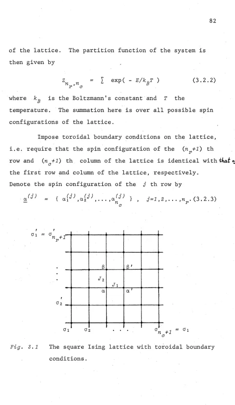
where kß is the Boltzmann's constant and T the temperature. The summation here is over all possible spin configurations of the lattice.

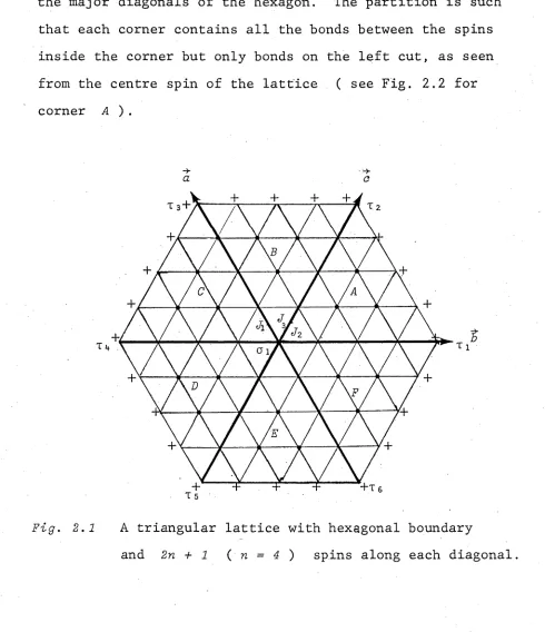
lattice into six "corners" ( A to F ) with three cuts along the major diagonals of the hexagon. The partition is such that each corner contains all the bonds between the spins inside the corner but only bonds on the left cut, as seen from the centre spin of the lattice ( see Fig. 2.2 for corner A ).

T 5

Fig. 2.1 A triangular lattice with hexagonal boundary

and 2n + 1 ( n = 4 ) spins along each diagonal. In a similar way to Baxter (1976), we divide the

+

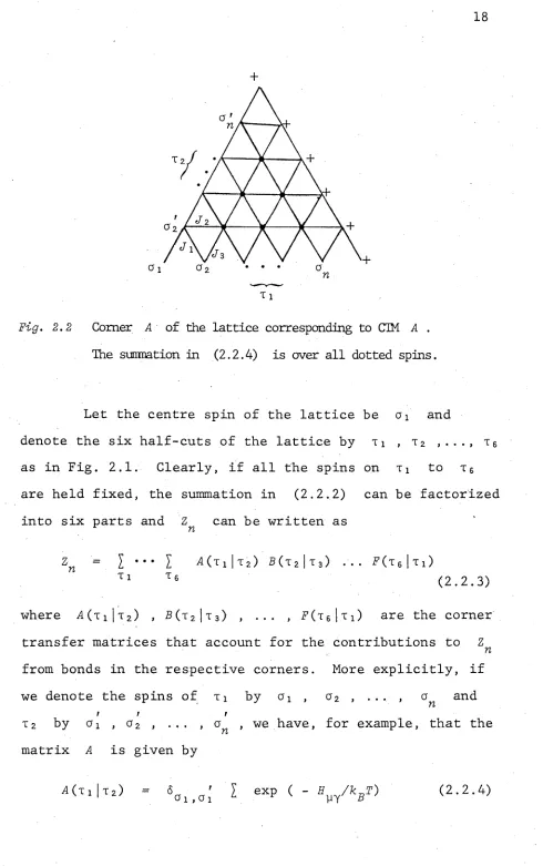
Fig. 2.2 Comer A of the lattice corresponding to CTM A .

The sumnation in (2.2.4) is over all dotted spins.

Let the centre spin of the lattice be oi and

denote the six half-cuts of the lattice by Ti , t2 t6 as in Fig. 2.1. Clearly, if all the spins on Ti to t6 are held fixed, the summation in (2.2.2) can be factorized into six parts and Z can be written as

r n

Zn = i ••• I 4 ( T ! I T 2) B( T 2 |t3) ... F(t 6 I T 1 )

Tl Te (2.2.3)

where 4 (t i|t2) > F (t2 |t3) , ... , F(t6 |t i) are the corner transfer matrices that account for the contributions to Z

n from bonds in the respective corners. More explicitly, if we denote the spins of Tj by a x , a2 , ... , and

r r t

T2 by ai , a 2 , ... , a , we have, for example, that the matrix A is given by

I exp ( - H ^ / k BT)

where H^ is the interaction Hamiltonian involving all the bonds of the corner and the summation is over all interior

spins of the corner as shown in Fig. 2.2.

Furthermore, it can be seen readily that the matrix D is the same as A , E as B , and F as C . Hence

(2.2.3) can be written as

Z = Trace ( ABC )2 . (2.2.5)

n

We further note that B is obtained from A by replacing Ji by J 2 , Jz by J3 and J3 by Ji . Similarly C is obtained from A by replacing Ji by J3 , J3 by J 2 and J2 by J i .

In the thermodynamic limit, the partition function per site is given by

Z = lim Z 1/N (2.2.6)

n oo

where N is the total number of sites in the lattice and the free energy per site f is

k T

f = -lim -2- In Zn (2.2.7) n->°°

Also, the spontaneous magnetization M is just

< g i > Trace { S(ABC) }

Trace { (ABC)2 }

(2.2.8)

where

t t

S( oi,...,on I o l, ...,on ) G i 6 ' 6 '

o 1 > 0 1 O 2 , O 2

. 6 G , G

is the diagonal centre-spin operator. Since the matrices A , B and C all break into two diagonal blocks

corresponding to Oj = fl or -1 , they commute with the diagonal matrix S .

The trace of a matrix is simply given by the sum of all its eigenvalues and therefore by (2.2.5) , the problem of evaluating the partition function reduces to finding the eigenvalues of the product of the corner transfer matrices ABC .

The following arguments will be mainly focussed on the analysis of the CTM A . Those for B and C may be obtained similarly by making the necessary changes of the parameters involved.

§

2,2

To further simplify the corner transfer matrices, we would like to decompose them into row matrices in a similar way as for the square lattice (Baxter, 1976).

We consider a more symmetric corner which includes the bonds on both of the cuts and denote it by A' for corner A and similarly B' and C' for corners B and C respectively. Denote

Obviously, the new corner transfer matrix A ' is

related to CTM A through

A = La A ' (2.2.11)

where L A is the matrix which cancels the effect of the

added bonds, or, more explicitly

V ai’°2... °n

t i r h , a 2 , . . .

,on

{ exp [- K 2 (o iO 2+o2o 3 + - • •+o o .-)]} 6 '...6 ' K L n n+1 J ai,ö! o2 ,o2 °n >°n

(2.2.12)

with a , = 1 . n + 1

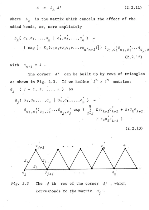
The corner A ' can be built up by rows of triangles

as shown in Fig. 2.3. If we define 2n x 2n matrices

G. ( j = 1 , 2 , . . . , n ) by J

G A h >o2 ,...,on

6 '6 '

öl ,Ö1 O 2 , O 2

t t t

a i ,a2,...,

6 ' exp {

a ., a . r

)

Kl0 SL+l°$L+l + Kz°l°Sl + l

1=0

+ K * °l\ + 1 }

(2.2.13)

t t

The j th row of the corner A 1 , which corresponds to the matrix G . .

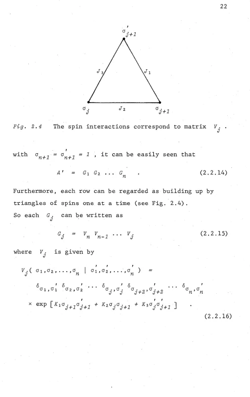
Fig. 2.4 The spin interactions correspond to matrix 7. .

with

°n+l °n+l 1 it can be easily seen that A' = G l G2 ... G

n (2.2.14)

Furthermore, each row can be regarded as building up by

triangles of spins one at a time (see Fig. 2.4).

So each G . can be written as

0

G . = V V * ... V. (2.2.15)

«7 n n-1 o

where V . is given by J

V . ( 0i,ö2 ,...,o

j n

1 t r

ö i , a2 , . . . , cr^ )

6 ' 6 ' ... 6 ' 6 '

01)01 G 2 ’° 2 ° 0 > ° C ° j + 2 > ° j + 2

6 a , a

n n

§

2.3

We introduce a set of Pauli spin operators in terms of which all the v s can be conveniently expressed.

Denote the three familiar anticommuting 2 x 2 Pauli spin matrices by

(where i = /-I )

d

(

.

.

)

a n d d e f i n e t h r e e c o r r e s p o n d i n g s e t s o f 2

s . , q . a n d

J J d i ( J' =

2, . .. . ^ n ) a s

s . = J

I 2 © I 2 © . . ,. © s © . . . © 12

c . =

J

I 2 © I 2 _{© . . . © (3 © .. . © 1}2

III

^

3

I 2 © I 2 © . . . © d © . . . © I 2 1

j t h f a c t o r

x 2n matrices, follows

( n factors ) ( n factors ) ( n factors )

(

.

.

)

where I is the m x m identity matrix and © denotes the direct product of the matrices.

One can easily verify that a given j ( j = 13 2, . . . , n )

s .

C o .J and d .J for

(i) are anticommuting with each other, i.e.

s .

J c .J + o .J s .J = 0

e .

J d .J + d •<7 e .J = 0

d •

J s .J + s .J d .J = 0

whereas they commute with any other matrix of the

sets of operators;

(ii) satisfy the following relations

2 2

S . = C . =

J J d 2 J = I (2.2.20)

s • c . = i d . ;

J J 0 o .0 d .3 = i s .3 ; d .3 s .J = i

(2.2.21)

§

2.4

o . .

3

In order to express the matrices in terms of the spin

operators defined in Section II.2.3, we further decompose V .

0

into a product of three matrices. From (2.2.16) , we have

7. = R (.2) Y (.1) R (3)

0 0 0 0 (2.2.22)

where

(i) I r > I

R • ( o i, o 2 , . . . , a I o i , a 2 , . . . , o )

6 ' <5 '

O 1>0 1 CT 2 ,O 2 6 a ,a _{n ’ n}' exp ( ^ v K no .o .£ j J-/-2 ) and

(i) ' ' '

F . ( oi,o2,...,a I 0 1 , 0 2 , . . . , o „ )

&°u°i&°2,Oz---Soj ,o'.öo;j+2,o[+2---Son ,o^ ®*P ( V jViV j }

i = 1, 2, 3

3 = 1 , 2, n-i .

It may be noted that for any matrix X whose square is the unit matrix, the following identity holds :

exp ( Q X ) = cosh 9 + X sinh 0 (2.2.24)

for any scalar 0 . Hence, it is obvious that

exp ( K n s . s . )

& J o + l (2.2.25) and by equating elements, we have

= ( 2 sinh 2K£ )^ exp ( K* c. + 1 )

1, 2, 3

7 , 2 , . .. , n-1

(2.2.26)

where

tanh K exp ( - 2 K 0 ) , 1 = 1 , 2, 3 . (2.2.27)

Hence, we may write

= (2 sinh 2 K lY 2 e x p(K2s .q .+ ^). e x p .+ J) e x p(K3s j.s^+1 )

J = 7, 2, ..., n-7

and also

I,

s = 1

n + 1

(2.2.28a)

Vn = exp ( £ 2 ) exp ( K 3 ) . (2.2.28b)

Similarly, L can be written as

(2.2.29)

form

7 . 3

where

% U f + 9 ) + tf-g)s.s.+1 + (h+r)c.+1 + (h-r)s.s.+1e.+1]

(2.2.30)

f = exp ( Ki + K z + K

9 = exp ( K l - K 2 - K

h = exp _{( - K i + K 2 - K}

r = exp _{( -} - K 2 + K

(2.2.31)

The form is similar to that obtained for the square lattice

Ising model (Baxter, 1977).

Hence, all the corner transfer matrices can be

written as a product of matrices of the type exp ( xs )

and exp ( yo . ) . In fact, it is one of the delightful

properties of the Ising model that in the absence of the

magnetic field, all the 2 x 2 matrices that occur have

this structure. As will be shown in the next section, this

The problem now is to diagonalize the CTMs A , B and C . In Section II.2, we have shown that, in the absence of a magnetic field, all the matrices that occur in the model are of the type exp ( xs .s . ) , exp ( yo . ) and their

J J 0

products. It was illustrated by Kaufman (1949) that all such matrices form a 2 -dimensional representation of the group

of rotations in 2 n -dimensions and hence they can be represented by 2n x 2n matrices. As a result, we may equivalently work on the representation of the CTMs in this 2 n -dimensional rotational space.

§

3,1

We study here the relations between the

2 n -dimensional rotation ( i.e. orthogonal matrix ) and the corresponding 2 -dimensional matrix in the spin representation.

Given a set of y operators, Y. of dimensions

0

Yl Yl

r .

o

o

y

(2.3.1)

ihe set of all non-singular 2n x 2 n matrices X

such that

_ 7

X r

0

I

£ • “ .£ J , £ J

(2.3.2)

for some £ . ^ , forms a group . The y x y matrix with

elements x ^ is called the representative of X and is

A

denoted by X . The representatives have the following

properties

(i) From the anticommuting properties of the r . , each

0

representative of the group is orthogonal.

Furthermore, each representative determines its parent

matrix to within a multiplicative constant.

(ii) If X\, X 2 , X . t Y are members of the group ^

such that X i X z - ' - X . = Y then the corresponding J

representatives Xi, X 2 , •••, X ., Y satisfy the same

J

relationship, i.e. X \ X 2 . . . X . = Y . J

In order to formulate our problem in this spin

representations, we define a set of 2n anticommuting

operators by

d c l s2

r 2j - I a 1o 2 . . . a . _ 1 _{V 2j} C l O 2 . . . C . 8 . 1 , 1 , 2 , . . . , n . (2.3.3)

where s. , u. and d. are the Pauli spin operators acting

on the j th spin as defined in (2.2.18), and sn+-j i-s the identity matrix.

With this set of operators, for any X in the group formed by the transformation in (2.3.2), we may further establish the following properties on the representatives :

(iii) If X is real and symmetric, then X is Hermitian and

X n = JL X j[^ (2.3.5)

where * here denotes the complex conjugate of the matrix and ^ is a 2 n x 2 n diagonal matrix with

elements

J

L

-

-1

J ) J

(2.3.6)

__ /\

(iv) If X is real and orthogonal, then X is real and

1 = <4 X JL . (2.3.7)

This implies that X is built up of 2 x 2 diagonal subblocks.

(v) If X is diagonal, it must be of the form

X const, x n % [ ( 7 t p . ) + ( l - p . ) s . s . ]

0 J 3 + 1

(2.3.8) for some scalars p . ( j = 1, 2 , . . . , n ) and X is

3

^ i

A 2

X =

A . 3

(2.3.9)

where A . are 2 x 2 orthogonal m a trices and can be w r i t t e n as

A .

3 %

, -1

p . + p * i (p:-3 - P •) \

3 3 3 3

-i (p"-7 - P •) P- t p'-7 )

J 3 3 3

3 = 1 , 2 , . . . , n

(2.3.10)

( i = / - : ) .

§

3.2

We are n o w ready to express the corner transfer mat r i c e s in terms of spin representation.

It can be v e r i f i e d that all the matrices V . and 3

defined in (2.2.16) and (2.2.12) belong to the

group m e n t i o n e d above. Using the set of operators defined in (2.3.3) , we find that

(i) r, r ' / * - 1 =

“ V2j-1 1 g V2j '

1~H 1 •^ > CK 1 II <=> ? 4-1 • H =

l2j-l + “ r 2j ’ if * = 2j

=

h otherwise .

(ü)

( i ü )

w h e r e

/\

V .

3

E (S>

3 r £ e3(.3) = cl’T2j-l " l ß 'r 2j ’ i f

T-S

1

cv

i

II

<=>

?

i 3 '

r 2 j - 2 + a 'r 2j ’ i f £ = 23

r £ > o t h e r w i s e

( 2 . 3 . 1 1 b )

a n d

Y ( V 3

(1 ) ~ 2

r 0 i .

£ 3 = Y r 2j 1 6 r 2 j + r i f £ = 2 j

= i 6

r 2j + 7 T2j + 1 > i f £ = 2 3+I =

r £ > o t h e r w i s e

( 2 . 3 . 1 1 c )

Y = c o t h 2K1 } 6 = c o s e c h 2K\

a = c o s h 2 £ 2 ₎ 3 = s i n h 2K2 ( 2 . 3 . 1 2 )

a ' = c o s h 2 Z 3 } 3' = s i n h 2K3

H e n c e , f r o m ( 2 . 2 . 2 2 ) , V . i s s i m p l y g i v e n by

3

23-1

23

2j + l

23-1 23 23 + 1

a a ' - f 3 3 ' y i ( a $ ' - f a ' 3 y ) - 3 6

- i ( a ' 3+063 ' y) 3 3 , TLota, Y i a 6

- 6 3 ' - i a '6 y

and from (2.2.29) ,

a _-iß 0 0

13 a 0 0

0 0 a -13 (2.3.14)

0 0 13 a

Hence the CTMs A , B and C are also members of the group ( i.e. their representatives under T. exist ).

5 4 , 1 THE CTMS AND THEIR REPRESENTATIVES

Before we continue our analysis, we observe that

the CTMs A , B and C ( hence their representatives ) do not necessary commute with each other for arbitrary

Ji , J2 and J3 . However, our aim is to diagonalize the matrix

representatives (Section II. 3.1), this is equivalent to

A

finding a similarity transformation which brings $ to a block diagonal form. We have

*9

i.e. to look for a matrix, say P 2 , such that

P i 1 $ P i = c ö d (2.4.2)

where oOj is a diagonal matrix. From property (v) of the

A 2

< & d = 2 (2.4.3)

X .

c

Since pQ and oD^ are orthogonal matrices, one can choose

^ A . A /\

P2 to be orthogonal also. As A , B and C are all

orthogonal matrices, we may define orthogonal matrices

Pi and P 3 such that

A -7 A P 2 4

A P 3 =

/\

(2.4.4a)

A -1 A

P3 5

/N

Pi = _{B d} (2.4.4b)

A -7 A

Pi c

A

P2 =

/\

cd (2.4.4c)

and require that

/V. /S

^ - s

/\

^ and C^ are all orthogonal and

of block diagonal form.

/N

For example, A^ is given by

^ l(1)

(1) x (1> 0 (2.4.5) where J ^ /\

Bj and C,

a a

respectively.

are 2 x 2 orthogonal matrices, similarly

with A r e p l a c e d by A ^ and x(2/)

J ^ J J J

Obviously, we then have

for

Bd c d .9d (2.4.6)

A

Note that from the set of equations (2.4.4a-c), Pi is a

A A A /\

matrix which diagonalizes the matrix CAB and P3 a matrix

/ \ / \ /N

From prpperties (i) and (ii) of the representatives, the corresponding matrices in of the representatives

/ \ ^ /\

, B £ , Cd and P^ can be chosen to satisfy the set of equations (2.4.4a-c) also, i.e. we can find 2 x 2

matrices , C^ and P^ , i = 1, 2 , 3 in satisfying

P 2 1 A P 3

A d • BPl * B d ■ P ‘2

-(2.4.7) Also

A d B d C d

&

Hence, if we can solve (2.4.3) or equivalently (2.4.4a-c), we shall have obtained the diagonal form of q9

We now perform the analysis on the representatives. It is convenient to group the elements of the matrices A , /N /\

B , C a n d

\ < * 1, 2, 3 ) i n t o 2 x 2 b l o c k s a n d w r i t e

/\ A =

iai p ’ A B

= (bi P a n d A c =

{oi,p (2.4.9)

a n d /\ p i "

, U )

( ) , 1 = 1, 2 , 3 (2.4.10)

i , C = 1 , 2 > • • • ) n

w h e r e a . .

’ b a - G . .

A (l)

4 ( y ^ )

0 0

= I

1 , 3 = 1

i - l 3 - 1

a . . y z ( 2 . 4 . 1 1 a )

<& ( ^ x )

0 0

= I \ b . . _^>3 z i - l x3 - 1 ( 2 . 4 . 1 1 b )

& ( x 3 y )

T-H

II

8

II i - l 3 - 1

c . . x y ( 2 . 4 . 1 1 c )

and

v p ( x )

r m

0 0

= I

3 = 1

P ( l ) J - 1 , 1 = 1 , 2 , 3

m = 1 , 2 , ,. . . . ( 2 . 4 . 1 2 )

From ( 2 . 4 . 1 2 ) we ha v e

p ( l > = _{( 2i r i ) ~ J} S c

i

U )

,

p m ( y ) dlJ > 1 = 1 , 2 , 3

3 > rn = 1 , 2 , ,. . . . ( 2 . 4 . 1 3 )

where the contour of integration o is a simple closed curve surrounding the origin in the y plane within and

( £)

on which p . ( y ) is analytic. J

In view of equations (2.4.9) and (2.4.10) , the set of equations (2.4.4a-c) can be expressed in the form

00

1

1 = 1 a ir%

(3) p t,3

( 2 ) . ( 1 )

^

(2.4.14a)

00

1

1 = 1

h i x p (1>_{P 1,3}

(3) , ( 2 )

= p . . A .

^

00

1

J1 = 1 ° i X

pi2’.

P 1,3 = p i 1 ’.1 , 3 X (.S)0

(2.4.14c)

Hence, from (2.4.11a-c), (2.4.13) and (2.4.14a-c) , one

can easily arrive at the coupled integral equations

( 2 7T i) 1 I034 ( ( 3 ) , , dz/z

(2) , s . (1)

= ( y )

( 2 . 4 . 1 5 a )

( 2 TT i) ”1 _{\ C B (} ( 1 )s

P3 (X) dx/x = p ' i h s ) 0 y z>3 ( 2 . 4 . 1 5 b )

(2v±)-2 la £ f e y " 1 ) _Pj (2) ,_\y) v d y / y ( i ;

, s , rsj = p . (x) A .

3

(2.4.15c)

The main task reduces to solving these set of

coupled integral equations.

§

4.2

M

It is possible to evaluate the generating function

<A

1

o

Define matrices H ( r = 1, 2, . n ) by

(2.4.16)

We can evaluate H directly from (2.3.13) .

With w . , j = 0, 1, 2 and h . , g . , j = 0, 1, 2, ..., n

0 C J

being 2 x 2 blocks defined as follows :

w

o

-36

ia6

0

Wi

-63' -ia'6

0 0

h .

3 and

y o

o 1

aa '-f 88 'y

-i(a'3*a3 'y)

(2.4.17)

i (a3 '+0L' 3y)

88 ' +OL0L 'y

V 1

-68 ' (aa ' + 83 'y) -ia ' 6(aa ' +88 'y) i6 8 ' (a ' 8t*-068 'y) - a ’ 6 (a ' 8+a8 'y)

(-6 8')/ \ 3 1

h w 2 o

l > j = 1 , 2 n (2.4.18)

y(aa'iL8 8 ,y) i(a8'iLa'8y)

- i y ( a '8+a8'y) 88'*aa'y

0i /■z iW2

-68 ' Y (aa'-/-88 'y) -ia ' 6 (aa ' +88 'y)

i68 'y(a'8 + a 8 fy) - a '6( a '8+a8'y)

9j = ( - S ß ' ) ' 7' 2 gi ,

(2.4.19)

h w 0 0 0 0

0 0

hi

^0 wo 0 0 0

h z _9i

^0 w0 0 0

^3 92 9 i

f o • 0 0

// = •

r

• . • • • . .

?Z 7

r - 1 $ r - 2 &r-3 ^r-4 w0 0

r t h

b l o c k (-6 3 ')2 ~wi ( - ö $ ,) Pwfw 2 (-6 3 ')p wiW2 ( - 6 3 ' ) Pw t w 2 . . WiW2 w 2 0

0 0 0 0 . 0 0 I

r = 1, 2 n . ( 2 . 4 . 2 0 )

/ \ / \ A

H e n c e t h e m a t r i c e s H , H . , H . . . . . , h a v e

r r +1 r +2

t h e i r f i r s t 2 ( r - l) r o w s i n common a n d s o we e x p e c t e a c h e l e m e n t ( £ , m ) o f t e n d s t o a l i m i t a s r a n d n t e n d t o w a r d s i n f i n i t y .

I n v i e w o f ( 2 . 2 . 1 5 ) , we h a v e

Gi = Hn , ( 2 . 4 . 2 1 )

s o , i n t h e t h e r m o d y n a m i c l i m i t ( ) , we e x p e c t

G = l i m G l = l i m H . ( 2 . 4 . 2 2 )

n->°° n , r-^00

A l s o , n o t i n g t h e s t r u c t u r e o f V. f r o m ( 2 . 3 . 1 3 ) , we o b s e r v e J

t h a t f o r n = 00 ,

or equivalently using (2.2.14), we may write

(2.4.24)

To calculate the generating functions of the CTMs , we define

a matrix by

*1

12 0

6 3 f 1 2 1 2 0

0 6 3' I2 I2

0 6 3 f 12

0

(2.4.25)

and write (2.4.24) as

Note that

r’i a =

w 0 0

o

17li w 0

o

0 m m i w

o o

m o Wl

(2.4.26)

(2.4.27)

w h e r e

m = öß'/z f 1

0 0

m1 6 ß 'w + g

0 v0

I n a s i m i l a r way t o _{^ (2}

f 00

j4 ( y , z ) = I

1, 3 = 1

w h e r e (a ' .) a r e 2 x 2

e l e m e n t s i n ( 2 . 4 . 2 6 ) , T

e q u a t i o n s :

a l,l = h(

a* . = w

1

6ß- a ' 2 = m

1

+ a j u_> = 0

and

6 e ' _{* a ^ , j}■ ~

0 - i 6 a \

, 0 - 6 3 /

ß ß ' - f a a ' y i ( a ß '-/-a ' ßy) \

- i ( a ß 1+0L ' ßy) ß ß ' - f a a ' y /

( 2 . 4 . 2 8 )

ho

i - i i - i

( 2 . 4 . 2 9 )

o 1 , 0 - 1 3 = 2, 3,

l = 3 , 4 ,

( 2 . 4 . 3 0 )

a ! n . - -f »zi a / - . - + w a ! .

-o SL-2 , 0 - 1 k - 1 , 0 - 1 o 1 , 0 - 1

1 , 3 > 2 ( 2 . 4 . 3 1 )

£ - 1 7 - 7

M u l t i p l y i n g ( 2 . 4 . 3 1 ) by z/ 3 and summing o v e r

I

& , «7=2 K . J + 6B' ai-2.j

X l-l 3-1

) y z

+ + W o y

l-l 3-1

z

(2.4.32)

On simplification and using (2.4.30) also, this gives the r

generating function A (2/, a) as

. t _ 2

A Oj , z ) = ( 1 + 63 ' y - rn^y2z - ml y z - Wq 2 ) ( h Q + mQy )

(2.4.33)

It can be easily verified that

( 1 + 6ß'y - m^ y 2z - m i y z - w^s )-1

2 / l +&$,y - ( $ $ ,+a a ,y ) y z +6$ y 2z i y z (aß ,+a., $y-a.6y) '

(i-f6ß y) A ( y , z ) y -i[(aß '-fa fßy)y-a6]2 1+S$' y+S$z- ( $ $ ,+aoL,y ) y z i

(2.4.34)

with

A ( y , z ) = 1 + 2/ 6 ß f + s6ß - 2 y z (ßß '-faa ' y) + y 2 z S $

+ zy2 2 5 ß ' + y 2 z 2 (2.4.35)

where y , 6 , a , a' , ß and 3' are defined in (2.3.12). Note that if we put y = e^9 and z = e ^ , (2.4.35)

becomes

A(y , z ) = s \ " ( coshSKi cosh2£2 cosh2X3 +

sinh2#i sinhSX2 sinh2Z3 - sinh2i£2 cos0 sinhSXi cos(0-f(j)) - sinh2X3 cose}) )

The logarithm of the expression in brackets is just the integrand of the double integral for the free energy of the triangular lattice [ Temperley, 1950: Eqt. lo].

As for the generating function A (y ,z) , from (2.4.33)

A (y,z)

A (2/ ,z)

aa '-/-33 ry-yyz i (a3 '+a ' ^y-6ay) ■l(a'$+a & 'y-&a1z) 33 ' taa 'y - 6 3^-6 3 ' z

-yz

(2.4.37)

Using (2.2.11) and (2.3.14), we have

£, j where

I a ' . , Ü, 3 = 1, 2, . . .

a l

a - i3

i3 a

(2.4.38)

(2.4.39)

or equivalently, we may write

A ( y , z ) = A (y,z) • (2.4.40)

We have therefore in fact obtained the generating function

A(y,z)

(^ ,2)

_h(y

,

2

)

/ a ’ (l+z&$)-yzoci \ -i(3,yti/3 3y-2aa,6)

i{ 3'.(7+z6 3) +y z3-y 6 } a'y-,sa(ö3r+y)

(2.4.41)

Similarly, 'f6 (z ,x) and tS (x,y) can be evaluated

A A

explicitly. The elements of A ( and similarly B and

A

(y,z) ( respectively $ (z,x) and T? (x ,y) ) in powers of y and z .

§

4,3

To solve the coupled integral equations (2.4.15a-c), we apply the elliptic function parametrization which occurs

naturally for the triangular lattice as follows :

cosh 2K . 0

sinh 2 K .

J

cn(2v .)

3

- i sn(2v^.) , j = 1, 2, 3

(2.4.42)

where sn , cn and dn are Jacobian elliptic functions with modulus k given by (Stephenson, 1964) :

[U-*?)(2-tf)(2-tb]2

k 2 =

---1 6 (---1 + t it zt3 ) (t i+t zt s') 2 + t 3~k 1) 2 l ~fc2)

(2.4.43)

where t . = tanhX . , j = 1 . 2 , 3 .

J 3

Now if we restrict ourselves to the regime where all the K. are real and positive ( i.e. we consider only the

J

pure ferromagnetic case ), the v . will be all purely

J

imaginary and are subjected to the following conditions :

0 < Im(v.) < K'/2 and Vi + v 2 + v 3 = i K r/2

(These are not to be confused with the energy coefficients

K i , K 2 and K 3 used above.) If we apply the following

transformations to the variables of the integral equations

(2.4.1 5 a - c ) ,

x = k s n( ui+Vi) sn(ui-Vi)

y = k sn(u2t v 2) sn(u2-v 2) (2.4.44)

z = k sn(w3+ v 3) s n ( u3 - V 3 )

we can solve the equations in terms of the new variables

m i, u2, u 3 . It is more convenient to work on the new kernel defined by

W1 ( u2, M 3 ) du 3 = (y dz/z (2.4.45a)

C

O

3

C

M _.Wl) du 1 = _{(2,^~2) d x / x} (2.4.45b)

f/3 (m _{1 ,^2)} du 2 = 6 _{, y~ 2)} dz/A (2.4.45c)

We now restrict the analysis to ( y , z) •

We are able to factorize h ( y ,z ) in terms of the

variables u 2 and u 3 . Using the transformation given

in (2.4.44) and considering the sum and product of the

roots of the expression in (2.4.35) as a function of y ,

we obtain

_<2

2 2A(y, z ) = k 2 (2 - /c2sn(u3-Fvr3)sn(M3-V3)sn(2v2-/-2v3)sn(2v2))

x (sn(M2tv2)sn(M2-v2) - sn(u3-fv3)sn(u3-fV3+-2v2))

x (sn(w2-fv2)sn(u2-v2) - sn(M3-v3)sn(w3-v3-,2v2))

[Appendix IIB ] .

Similarly, we may obtain Wi(u2)u 3) as a function of u 2

and u3 . Consider the following matrix

-1

(w2 ,v2) M i (u 2 ,1^3) Z}(w3,v3)

where D(u,v) and M .( w .,«„ ) are

^ J & 2 x 2 matrices given by

D (u, v)

/ -cn(w-v) dn(u-fv) sn(w-v) \

\ cn(u-fv) sn(w-fv) dn(w-v) J

(2.4.47)

-*(yMÄ+vvÄ)

(2.4.48)

with

<f)(w) = dn(u)/sn(w) (2.4.49)

and i c l cyclic permutation of 1 2 3 .

It can be shown that this matrix has the same poles and

residues as f/i(w2 »w3) and hence by Liouville's theorem

and their periodicity, they are in fact the same matrix

[ Appendix IIA, B ] We may then write the kernels as

Wi <'uj'U%) = D k u - . v . ) M i {u.,ul) D(ul ,vl) (2.4.50)

where i j i are cyclic permutations of 1 2 3 .

The coupled integral equations (2.4.15a-c) become

<2lTi>’2 A ’

V V V

=

>(ui 47

^

m = 1, S, ... (2.4.51)

§

4.4

Before we proceed any further, we would like to comment on the contour of integration for the coupled

integral equations in (2.4.15a-c) and hence for (2.4.51). We would like to focus our attention on the z plane for

the integration of (2.4.15a) . Similar arguments can be applied to the integrations of (2.4.15b) and (2.4.15c) in the x and y plane respectively with necessary change of variables.

( 3 ) Suppose that the radius of convergence for p (z) , ( m = 1, 2, ... ) as defined in (2.4.12) is R

/N

orthogonality requirements for P 3 , we have

By the

J=1 P m ’l pLj = ’ K 3 = 1, 2, ... (2.4.52)

( 3 )

This implies that we must have p . -* 0 as l °° and

^ > J

so, the radius of convergence R cannot less than unity. The contour of integration c 3 must then be a circle of radius less than R and yet, it must be sufficiently large that j4t (y yz ^) is an analytic function of z for z

outside and on o3 .

is valid by choosing o 3 such that

(i) c 3 is a simple closed curve surrounding the origin; (ii) p^2{z) is analytic for z inside and on o 3 ; (iii) for y e D , both poles of (y,z ^) in the z

plane lie inside o 3 .

Under the transformation from z to u 3 , we find that provided

v 3 < n ' < iK ’ - v 3 (2.4.53)

we have

(i) a straight line with Im(u) = n ' maps to a simple closed curve c in the z plane surrounding the origin;

(ii) the domain v3 < |Im(w)| < n' maps to the interior of o ;

(iii) as u moves from left to right a distance 2K along the line Im(w) = r\' , z moves monotonically once around c in an clockwise-direction.

So, the contour of integration in the complex u 3 plane for (2.4.51) becomes a line segment (in3+ K ,ins-K) , where ri3 is such that the corresponding contour o 3 in

the original z plane surrounds the poles of the kernel &l (y,z ^) . An appropriate choice of H3 for (2.4.51) is

Using this, we may solve the coupled integral equations (2.4.51) in the complex u^ plane using Fourier