White Rose Research Online URL for this paper:
http://eprints.whiterose.ac.uk/137695/
Version: Accepted Version
Article:
Johnson, O, Aldridge, M orcid.org/0000-0002-9347-1586 and Scarlett, J (2019)
Performance of Group Testing Algorithms With Near-Constant Tests-per-Item. IEEE
Transactions on Information Theory, 65 (2). pp. 707-723. ISSN 0018-9448
https://doi.org/10.1109/TIT.2018.2861772
© 2018 IEEE. This is an author produced version of a paper published in IEEE
Transactions on Information Theory. Personal use of this material is permitted. Permission
from IEEE must be obtained for all other uses, in any current or future media, including
reprinting/republishing this material for advertising or promotional purposes, creating new
collective works, for resale or redistribution to servers or lists, or reuse of any copyrighted
component of this work in other works. Uploaded in accordance with the publisher's
self-archiving policy.
[email protected] https://eprints.whiterose.ac.uk/
Reuse
Items deposited in White Rose Research Online are protected by copyright, with all rights reserved unless indicated otherwise. They may be downloaded and/or printed for private study, or other acts as permitted by national copyright laws. The publisher or other rights holders may allow further reproduction and re-use of the full text version. This is indicated by the licence information on the White Rose Research Online record for the item.
Takedown
If you consider content in White Rose Research Online to be in breach of UK law, please notify us by
Performance of Group Testing Algorithms
With Near-Constant Tests-per-Item
Oliver Johnson, Matthew Aldridge, and Jonathan Scarlett
Abstract—We consider the nonadaptive group testing with N
items, of whichK=Θ(Nθ)are defective. We study a test design in
which each item appears in nearly the same number of tests. For each item, we independently pick L tests uniformly at random with replacement, and place the item in those tests. We analyse the performance of these designs with simple and practical decoding algorithms in a range of sparsity regimes, and show that the performance is consistently improved in comparison with standard Bernoulli designs. We show that our new design requires 23% fewer tests than a Bernoulli design when paired with the simple decoding algorithms known as COMP and DD. This gives the best known nonadaptive group testing performance for θ >0.43, and the best proven performance with a practical decoding algorithm for allθ∈ (0,1). We also give a converse result showing that the DD algorithm is optimal for these designs when
θ >1/2. We complement our theoretical results with simulations that show a notable improvement over Bernoulli designs in both sparse and dense regimes.
I. INTRODUCTION AND DEFINTIONS
In group testing, there is a population of items, some of which are ‘defective’ in some sense. We test subsets of items called ‘pools’. In the standard noiseless case we consider in this paper, a test outcome is negative if every item the the pool is nondefective, and is positive if at least one item is defective. Through many such pooled tests, we hope to be able to accurately estimate which items are defective.
The group testing problem was introduced by Dorfman [2], as described in [3, Ch. 1.1]. While a wide variety of problem setups have been considered, they all share common features, and can be considered in a wider class of sparse inference problems including compressed sensing [4]. Group testing has been applied in a wide variety of contexts, including biology [5]–[9], anomaly detection in networks [10], [11], signal processing and data analysis [12], [13], and communications [14]–[16] – although this list is far from exhaustive.
In this paper, we prove rigorous performance bounds for the nonadaptive noiseless group testing problem. ‘Nonadap-tive’ means that the make-up of every test pool is decided on advance, so tests can be performed in parallel. In the common Bernoulli design, each item is placed in each test independently with some fixed probability p. We instead
O. Johnson is with the School of Mathematics, University of Bristol, Uni-versity Walk, Bristol, BS8 1TW, UK. Email: [email protected]. M. Aldridge is with the Department of Mathematical Sciences, University of Bath, Claverton Down, Bath, BA2 7AY, UK, and the Heilbronn Institute for Mathematical Research, Bristol, UK. Email: [email protected]. J. Scarlett is with the Departments of Computer Science and Mathematics, National University of Singapore, 117417. Email: [email protected].
This work was presented in part at the 2016 IEEE International Symposium on Information Theory [1].
consider an alternative test design that we call the ‘near-constant column weight’ design. Here, independently for each item, we chooseLtests uniformly at random with replacement and place the item in those tests. We pair our design with practical algorithms for detecting the defective items. Using both rigorous asymptotic results and experimental simulations, we shall see that we can accurately detect the defective items with considerably fewer tests than the Bernoulli design.
We proceed by formalizing the problem and fixing some notation. We have a large number of itemsN, of whichKare defective. We assume that the defective items are rare, with
K =o(N) as N → ∞; moreover, for concreteness we follow [1], [17], [18] by takingK=Θ(Nθ)for some fixed parameter
θ ∈ (0,1). We follow the ‘combinatorial model’ and suppose thatK, the true set of defective items, is chosen uniformly at random from the NK sets of this size.
We perform a sequence of nonadaptive tests to form an estimateKbofK, and study the tradeoff between maximising the success probabilityP(Kb=K)and minimising the number
of testsT. We could simply takeT = N, and test each item one by one. However, Dorfman’s key insight [2] is that since the problem is sparse, in the sense thatK≪N, each test has a negative outcome with high probability, so these tests are not optimally informative. A better procedure considers a series of pools of items that are tested together, where the outcome of each test is positive if and only if it contains at least one defective item.
A group testing procedure requires two parts. First, a test designdescribes which items will be placed in which testing pools. Second, adecoding algorithmuses the results of these tests to estimate which items are defective.
Definition 1:We represent the testing pools by a (possibly random) binary matrix X ∈ {0,1}T×N, where x
ti = 1 if test
t includes item i and xti = 0 otherwise. The rows of X correspond to tests, and the columns correspond to items.
Definition 2: We consider the standard noiseless group testing model. The outcomes of each test are represented by a binary vector y=(yt) ∈ {0,1}T, where a positive outcome
yt =1 occurs if xti =1 for somei ∈ K, which is if the test
contains a defective item. A negative outcome yt =0 occurs
otherwise.
A commonly used test design is the Bernoulli design – see, for example, [17]–[23].
Definition 3:We define theBernoulli testing designas hav-ing a testhav-ing matrixXin which each entryxtiis independently
set to be1with probabilitypand0otherwise, for some fixed parameter p∈ (0,1).
In this paper, we will demonstrate that better performance can be achieved by using a design we call the near-constant column weight design.
Definition 4: We define the near-constant column weight testing designas having a testing matrixXin whichL entries
of each column of are selected uniformly at random with replacement and set to1, with independence between columns. The remaining entries ofXare set to0. We set L=νT/K for
some parameterν >0.
We now need an algorithm to produce an estimate of the defective set. In analogy with channel coding, we can think of the defective set K as a ‘message’ to be decoded from the ‘signal’ y, so we refer to such an algorithm as a ‘decoding algorithm’. (For more on connections between group testing and channel coding, see, for example, [4], [5], [17], [22], [24], [25].)
Definition 5:We estimate the defective set byKb=K(bX,y), and define the (average) success probability
P(suc)= 1
N K
Õ
|K |=K
P(Kb=K),
where the probability is over the random test design X.
We will demonstrate the superiority of our new design with two simple decoding algorithms. We define the algorithms here, but postpone detailed discussion to Section III. First, the COMP (Combinatorial Orthogonal Matching Pursuit) al-gorithm is a very simple alal-gorithm based on the fact that every item in a negative test is definitely nondefective.
Definition 6: The COMP algorithm is given as follows: 1) Mark each item that appears in a negative test as
non-defective, and refer to every other item as a Possible Defective (PD) – we writePDfor the set of such items. 2) Mark every item in PD as defective.
Second, the DD (Definite Defectives) algorithm builds on COMP to find items we can be certain are defective.
Definition 7: The DD algorithm is given as follows: 1) Mark each item that appears in a negative test as
non-defective, and refer to every other item as a Possible Defective (PD).
2) For each positive test that contains a single Possible Defective item, mark that item as defective.
3) Mark all remaining items as non-defective.
The main results of this paper concern rigorous bounds on the performance of the near-constant column weight design with various decoding algorithms. We are interested in how many tests are required for the success probability to tend to 1 as N gets large. Specifically, we show the following:
• The COMP algorithm requires 23% fewer tests with a near-constant column weight design than with a Bernoulli design, which for θ > 0.77 is fewer tests than required even for optimal algorithms with Bernoulli designs. (The-orem 2)
• The DD algorithm also requires23% fewer tests with a near-constant column weight design than with a Bernoulli design, which for θ > 0.43 is fewer tests than required even for optimal algorithms with Bernoulli designs, and for allθ∈ (0,1)is fewer tests than the best proven results
for practical algorithms with Bernoulli designs. (Theorem 3)
• We give an upper bound on the performance of near-constant column weight designs regardless of the decod-ing algorithm, showdecod-ing that DD is optimal for this design when θ≥1/2. (Theorem 4)
• We complement our rigorous theoretical results with sim-ulations that show a notable improvement over Bernoulli designs in both sparse and dense regimes. (Subsection II-C)
The structure of the remainder of the paper is as follows. In Section II, we define the rate of group testing (Subsection II-A), formally state our main results of the paper (Subsection II-B), provide simulation results to illustrate the improved performance of our test design (Subsection II-C), and briefly discuss some related work (Subsection II-D). In Section III, we describe the main decoding algorithms used in more detail and introduce some key quantities that control their performance. In Section IV, we deduce the main theorems of the paper, with proofs of some techinical results given the appendices.
II. FURTHER DEFINITIONS AND MAIN RESULTS
A. The rate of group testing
In this paper, we focus on nonadaptive designs, where the entire matrixXis fixed in advance of the tests. In the adaptive
case (where the members of each test are chosen using the outcomes of the previous tests), Hwang’s generalised binary splitting algorithm [26] recovers the defective set K using log2 NK +O(K) tests. This can be seen to be essentially
optimal by a standard argument based on Fano’s inequality (see for example [23]), a strengthened version of which [25] implies that any algorithm usingTtests has success probability bounded above by
P(suc) ≤ 2
T
N K
. (1)
This means that any algorithm with success probability
P(suc)tending to 1 requires at least
T =log2 N
K
∼Klog2 N
K ∼ (1−θ)Klog2N (2)
tests, where f(N) ∼g(N)means thatlimN→∞ f(N)/g(N)=1.
(See [21, Lemma 25] for details of the asymptotic behaviour of the binomial coefficient.) This motivates the following definition [21] of the rate of an algorithm.
Definition 8:For any algorithm usingT tests, we define the
rateto be
log2 NK
T . (3)
Given a random matrix design, we say thatRis anachievable rate if for any ǫ > 0, there exists a group testing algorithm with rate converging to R and success probability at least 1 −ǫ for N sufficiently large. We adopt the terminology
maximum achievable rate when referring to a given design (e.g., Bernoulli) and/or decoding rule (e.g., COMP).
In this language, the result of [26] shows that, for all
θ ∈ (0,1), adaptive group testing has an achievable rate of
R = 1 in the regime K = Θ(Nθ) and is therefore optimal, since by (1), no algorithm can learn more than 1 bit per test. It is an interesting question to consider whether there exists a matrix design and an algorithm with achievable rate
R=1 in the nonadaptive case. It appears to be difficult even to design a class of matrices with non-zero achievable rate using combinatorial constructions (see [3], [24] for reviews of the extensive literature on this subject, with key early contributions coming from [27]–[29]). Hence, much recent work on nonadaptive group testing has considered Bernoulli designs (see Definition 3). The maximum achievable rate is known exactly for such designs, as stated in the following.
Theorem 1: The maximum achievable rate for Bernoulli nonadaptive group testing with K = Θ(Nθ) defectives, for
θ∈ [0,1), is
C(θ)=max ν>0 min
ν e−ν ln 2
1−θ
θ ,h(e
−ν
)
, (4)
whereh(t)=−tlog2t− (1−t)log2(1−t)is the binary entropy function. In particular, for θ ≤1/3, the maximum achievable rate of Bernoulli designs is 1.
The direct part of Theorem 1 is due to [17] and the converse due to [19]. (The special case θ=0 is older [30].)
The curve (4) is illustrated in Figure 1 below. Forθ≥1/2, the paper [21] showed that (4) is achieved by the DD algorithm described above. However, for θ < 1/2, the algorithms known to achieve the bound (4) are based on maximising the likelihood or solving other difficult combinatorial problems, and cannot be considered as practical in a computational sense – see Section III-D for more details. For example, we describe the SSS algorithm in Definition 10 below, which achieves the bound of [19], but is impractical for large values of N andK.
B. Main results
Our main results concern improving on Theorem 1 by using a near-constant column weight design (Defintion 4). Recall that this design has a testing matrix X in which L = νT/K
entries of each column of are selected uniformly at random with replacement and set to 1, with independence between columns, and the remaining entries of X are set to 0. The
tester may choose Lto depend on the parameters of the group testing problem.
Since the tests are chosenwith replacement, some columns may actually have weight slightly less than Ldue to the same test being picked more than once, hence we use the term ‘near-constant’. Since the weight of a column is the number of tests an item is in, we also consider these designs as ‘near-constant tests-per-item’. In a preliminary report [1], we used the less precise terminology ‘constant column weight’ for these same designs. Evidence from simulations and heuristic calculations suggest that truly-constant column weight designs have the same performance as the near-constant designs we consider
here, but the rigorous analysis of such designs seems more difficult.1
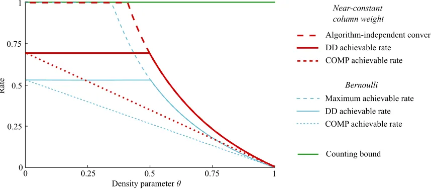
The main results of this paper are the following three theorems. The COMP and DD algorithms were defined in Defintions 6 and 7 and are discussed further in Section III. The main results are proved in Section IV. We illustrate these results in Figure 1, with our new rates for near-constant column weight designs marked in thick red, and corresponding rates for Bernoulli designs marked in thin blue.
Our first result concerns the simple and practical COMP decoding algorithm (see Defintion 6 and Subsection III-A), based on the fact that all items in negative tests must be negative.
Theorem 2: Consider a near-constant column weight de-sign with an optimised parameter ν > 0. When there are
K = Θ(Nθ) defectives for θ ∈ [0,1), the COMP algorithm has success probability tending to1 ifT ≥ (1+ǫ)TCOMP, and
tending to0 ifT ≤ (1−ǫ)TCOMP. Here
TCOMP= 1
ln 2Klog2N.
Hence, the COMP algorithm has maximum achievable rate ln 2(1−θ)for allθ∈ [0,1).
This rate
ln 2(1−θ) ≈ 0.693(1−θ)
is an improvement by30.6%on the rate 1
e ln 2(1−θ) ≈ 0.531(1−θ)
for COMP with a Bernoulli design [19], [23]. (An improve-ment in rate of30.6%corresponds to using23.4%fewer tests.) Further, forθ >0.766, Theorem 2 is an improvement on (4), meaning that in dense cases, the very simple COMP algorithm with a near-constant column weight design beatsanydecoding algorithm with a Bernoulli design (see Figure 1).
Some insight on this result can be attained by considering the conditions under which COMP succeeds. Under the choice
ν =ln 2, Bernoulli testing with probability ν/K and a near-constant column weight design with L = νT/K both result in roughly half of the tests being positive (e.g., see Lemma 1 below). However, a given non-defective item is placed in roughly Binomial T2,ln 2K negative tests under Bernoulli testing, and Binomial TKln 2,12 negative tests under the near-constant column weight design. While these two distributions have the same expectation, the latter has a much smaller probability of being zero, which is the event under which COMP fails.
It is also interesting to note that while ν = ln 2 (which is ’maximally informative’ in the sense of maximising the entropy of the test outcome) optimises the rate of COMP (as well as DD below) for the near-constant column weight design, COMP [23] and DD [21] with Bernoulli designs are optimised with a fraction1−e−1≈0.632 of positive tests.
1As pointed out by a reviewer, the COMP rate in Theorem 2 can be shown
Maximum achievable rate DD achievable rate COMP achievable rate
0.25 0.5 0.75 1
0 0.25
0.5 0.75 1
0
Density parameter θ
R
at
e
Bernoulli Near-constant column weight
Algorithm-independent converse DD achievable rate
COMP achievable rate
[image:5.612.89.518.56.244.2]Counting bound
Fig. 1. Rates and bounds for group testing algorithms with Bernoulli designs and near-constant column weight designs. In thick red, we plot the rate bounds for near-constant column weight designs from Theorems 2, 3 and 4. In thin blue, we plot the rate bounds for Bernoulli designs from Theorem 1 and [21]. The green horizontal line represents the universal ‘counting bound’ arising from (1).
Our second and most important result concerns the practical DD decoding algorithm (see Definition 7 and Subsection III-B).
Theorem 3:Consider a near-constant column weight design with an optimized parameter ν > 0. When there are K =
Θ(Nθ)defectives forθ∈ (0,1), the DD algorithm has success probability tending to1 if
T ≥ (1+ǫ) 1
ln 2max
Klog2
N
K,Klog2K
,
and hence has an achievable rate
R=ln 2 min
1,1−θ θ
=
ln 2 θ≤12
ln 21−θ
θ θ >
1 2. This rate
ln 2 min
1,1−θ θ
≈ 0.693 min
1,1−θ θ
is an improvement again by 30.6%on the rate of 1
e ln 2 min
1,1−θ θ
≈ 0.531 min
1,1−θ θ
proved by [21] for DD with Bernoulli designs. In fact, to our knowledge, DD with the near-constant column weight design gives the highest proven practically achievable rate for all
θ∈ (0,1). Further, forθ >1/(1+e(ln 2)2) ≈0.434, Theorem 3
is an improvement on (4), meaning that in this regime, the practical DD algorithm with a near-constant column weight design beats any decoding algorithm (even impractical ones) with a Bernoulli design.
Our third result is an algorithm-independent converse, show-ing the maximum possible rate of any decodshow-ing algorithm with a near-constant weight design.
Theorem 4:Consider a near-constant column weight design, with K =Θ(Nθ) defectives for θ ∈ (0,1). Regardless of the choice ofν >0, no algorithm can achieve a rate greater than
min
1,ln 21−θ
θ
=
1 θ≤θ∗
ln 21−θ
θ θ > θ
∗, (5)
where
θ∗= ln 2
1+ln 2≈0.409.
Comparing Theorems 3 and 4, we see that if we use a near-constant column weight design, the DD algorithm gives the optimal performance forθ≥1/2.
C. Simulations
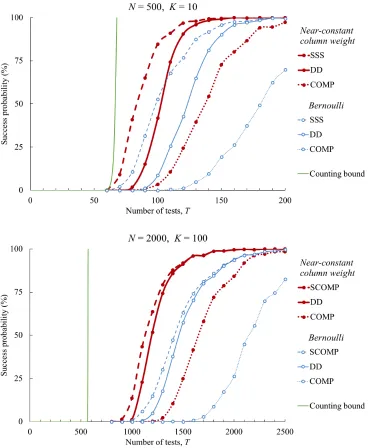
We complement our rigorous results on the rate, which are asymptotic as N → ∞, with simulations that show near-constant weight designs also improve on Bernoulli designs for finite problem sizes. In Figure 2, we illustrate the performance of these algorithms via simulations in an illustrative sparse case (N = 500, K = 10) and a denser case (N = 2000,
K = 100). For the sparse case, in addition to plotting performance of COMP and DD, we plot the performance of the SSS algorithm (see Definition 10), which achieves the bounds of Theorem 1 [20, Corollary 4], though is not practical for larger problems. Because of this issue of practicality, we do not consider SSS for the denser case; instead, we plot the performance of a related algorithm called SCOMP, which is described in [21], so we omit a description in this paper for the sake of brevity. (Essentially, it amounts to performing DD followed by greedy refinements.) Our near-constant weight designs provide a consistent notable improvement on Bernoulli designs, particularly in the denser example.
D. Related work
Fig. 2. Empirical performance (each point based on 1000 simulations) of various algorithms for both near-constant column weight and Bernoulli designs, in the casesN=500,K=10andN=2000,K=100.
have been proposed. Our key contribution is arigorous analy-sis of such designs in the regimeK =Θ(Nθ), requiring several novel techniques. In particular, we prove the achievability of rates strictly above those achieved by Bernoulli designs.
Kautz and Singleton [31] observed that a construction based on a concatenation of constant-weight codes gives matrices with the so-called K-disjunctness property (the union of any
Kcolumns does not contain any other column). Such matrices give group testing designs guaranteeing that K defectives can be recovered with zero probability of error in noiseless group testing (see for example [3, Chapter 7]). However, the group testing designs resulting from the construction of [31] require
T =O(K2(logN)2) tests. This is an example of the fact that the zero-error criterion requires considerably more tests than theT =O(KlogN)required for the ‘error probability tending to zero’ criterion (see Definition 8) that we study here.
Similarly, other subsequent papers have proposed forms of constant or near-constant column weight designs [32]– [35], but to our knowledge, none of these works provide non-trivial achievable rates for the vanishing error probability criterion, which is the focus of the present paper. Chanet al.
[23] considered constant row weight designs, and found no improvement over Bernoulli designs.
M´ezardet al.[36] considered randomised designs with both constant row and column weights, and with constant column weights only. The paper used heuristics from statistical physics to suggest that such designs may beat Bernoulli designs. In our notation, they suggest the maximum achievable rate of these constant weight designs may be equal to our converse bound (5) for allθ. (Our Theorem 3 rigorously proves this for
of a ‘no short loops’ assumption that is only verified forθ > 56
and conjectured forθ > 23, while experimentally being shown tofailfor smaller values such as θ= 13.
D’yachkov et al. [37] studied list decoding with (exactly) constant column weight designs, and setting their list size to1 corresponds to insisting that COMP succeeds. However, they only considered the case thatK =O(1). In the limit asK gets large, the rateln 2obtained [37, Claim 2] matches the rate for COMP given here in Theorem 2 in the limit θ→0.
A distinct line of works has sought designs that not only require a low number of tests, but also near-optimaldecoding complexity(e.g.,Kpoly(logN)) [38]–[41]. However, our focus in this paper is on the required number of tests, for which the existing guarantees of such algorithms contain loose constants or extra logarithmic factors.
III. DECODING ALGORITHMS:FURTHER DETAILS
In this section we discuss the COMP and DD algorithms in more detail, and introduce the SSS (Smallest Satisfying Set) algorithm. We discuss the conditions under which these algorithms succeed. These algorithms were previously studied in [23] and [21] with Bernoulli designs. Before continuing, we present another key definition:
Definition 9: Consider an item i and a set of items L not including i. We say that item i is maskedby L if every test that includes i also includes at least one member of L.
A. COMP algorithm
Recall the COMP algorithm from Definition 6:
1) Mark each item that appears in a negative test as non-defective, and refer to every other item as a Possible Defective (PD) – we writePDfor the set of such items. 2) Mark every item in PD as defective.
This is based on a simple inference: Any negative test only contains non-defective items, so any item in a negative test can be marked as non-defective. Given enough negative tests, we might hope to correctly infer every member ofKcin this way. The name COMP (Combinatorial Orthogonal Matching Pur-suit) was coined in [23], although the method itself appeared much earlier – see, for example, [5], [24], [31], [42].
Clearly, the first step will not make any mistakes (every item marked as non-defective will indeed be non-defective), so errors will only occur in the second step. As a result COMP will always estimateK by a setKbCOMP withK ⊆KbCOMP.
As in [21], a quantity of particular interest is G:=|PD \
K | = |PD| −K, the number of non-defective items masked
by the defective set K. SoG is the number of non-defective items that do not appear in any negative test. It is clear that COMP succeeds (recovers the defective set exactly) if and only if G=0, so that
PCOMP(suc)=P(G=0). (6) We use this in the proof of Theorem 2 in Section IV.
B. DD algorithm
Recall the DD algorithm from Definition 7, which builds on COMP to find items that are definitely defective:
1) Mark each item that appears in a negative test as non-defective, and refer to every other item as a Possible Defective (PD).
2) For each positive test that contains a single Possible Defective item, mark that item as defective.
3) Mark all remaining items as non-defective.
The performance of the DD algorithm with Bernoulli designs was studied in detail by Aldridge, Baldassini and Johnson [21]. Again, the first step will not make any mistakes, and since every positive test must contain at least one defective item, the second step is also certainly correct. Hence, any errors due to DD come from marking a true defective as non-defective in the third step, meaning that the estimateKbDD satisfiesKbDD⊆ K. The choice to mark all remaining items as non-defective is motivated by the sparsity of the problem, since a priori an item is much less likely to be defective than non-defective.
We analyse DD rigorously in Section IV, using the follow-ing notation, used in [21]. For eachi∈ K, we write:
• Mi for the number of tests containing defective item i and no other defective;
• Li for the number of tests containing defective item i and no other possible defective item (no other member of PD).
In the terminology of Definition 9, we see that DD succeeds if and only if no defective itemi∈ K is masked byPD \ {i}. Further, since item i is masked by PD \ {i} if and only if
Li =0, we can write
PDD(suc)=1−P Ø
i∈K
{Li =0}
!
. (7)
For a given defective itemi ∈ K, we writeK(i)=K \ {i} for the set of defectives withi removed. For a given set M, we write W(M) for the total number of tests containing at least one item from M. The random variable WK\{i} (the total number of tests containing at least one item in K(i)), henceforth denoted byW(K\i), will be of particular interest.
To understand the distributions of these quantities, it is helpful to think of the process by which elements of the columns are sampled as a coupon collector problem, where each coupon corresponds to one of theT tests. For a single item,W({i})is the number of distinct coupons selected whenL
coupons are chosen uniformly at random from a population of
T coupons. In general, for a setMof sizeM, the independence of distinct columns means thatW(M) is the number of distinct coupons collected when choosing M L coupons uniformly at random from a population ofT coupons.
Hence, as described in more detail in Section IV, we can first give a concentration of measure result for W(K\i) (see Lemma 1), then characterise the distribution of Mi given
C. SSS algorithm
We describe one more algorithm, which we call the SSS (Smallest Satisfying Set) algorithm, following [21]. This algo-rithm is not directly mentioned in the statement of our main results, but its analysis will be important in proving Theorem 4.
Definition 10: We say that a putative defective set J is
satisfying if:
1) No negative test contains a member of J.
2) Every positive test contains at least one member of J.
The SSS algorithm simply finds the smallest satisfying set (breaking ties arbitrarily), and takes that as the estimateKbSSS. Note that the true defective set K is certainly a satisfying set, and hence SSS is guaranteed to return a set of no larger size, so |KbSSS| ≤ |K |. However, it may not be the case that
b
KSSS ⊆ K. We can identify a particular failure event for SSS: If a defective item i ∈ K is masked by the other defective items K \ {i} (in the sense of Definition 9) then K \ {i} will be a smaller satisfying set, so SSS is certain to fail.
Hence, writing Ai for the event that item i is masked by K \{i}, we can use the Bonferroni inequality to obtain a lower bound on the SSS error probability PSSS(err)of the form
PSSS(err) ≥P Ø
i∈K
Ai
!
≥Õ i∈K
P(Ai) −1 2
Õ
i,j∈K
P Ai∩Aj.
(8) This serves as a starting point for upper bounding the rate of the SSS algorithm, which in turn will be used to infer our general converse (Theorem 4).
D. Note on practical feasibility
We refer to COMP and DD as ‘practical’ algorithms, since they can be implemented with low run-time and storage. For example, COMP simply requires us to take one pass through the test matrix and outcomes, requiring no more than
O(N) storage beyond the matrix itself, and O(T N) runtime. Similarly, DD builds on COMP, requiring two passes through the test matrix and outcomes and can be performed with the same amount of storage and runtime.
In contrast, we can interpret SSS as an integer programming problem, meaning that it is unlikely to be practical to run for large problems. We think of it as the ‘best possible’ algorithm without knowingK, and use a rigorous form of this statement [19] to obtain algorithm-independent performance bounds. Note that although the SSS algorithm may be considered to be infeasible in practice, the papers [43], [44] show that a relaxation of the integer programming problem to the real numbers can give good performance.
Furthermore, the decoding algorithms we consider here do not require exact, or even approximate, knowledge ofK. This is in contrast to the optimal maximum likelihood decoder of [17], which requires the exact value of K. Note, however, that the optimal choice of the parameter ν = (ln 2)T/K in the designstage does require knowing K.
IV. PROOFS OF MAIN RESULTS
The main goal of this section is to prove our achievable rate for the DD algorithm (Theorem 3). Along the way, we will also prove the COMP rate (Theorem 2) and the algorithm-independent upper bound (Theorem 4); the former will essentially come ‘for free’, though the latter will require non-trivial additional effort.
A. Concentration of W(M)
Recall thatW(M)corresponds to the total number of tests in which items fromM are placed. The following lemma shows that this quantity concentrates around its mean.
Lemma 1: Let M =|M|, and fix the constants α > 0 and
ǫ ∈ (0,1). When making L M =αT draws with replacement from a total ofTcoupons, the total number of distinct coupons
W(M) satisfies
P W(M)− (1−e−α)T≥δ ≤2 exp
−δ 2
αT
(9)
forT sufficiently large.
Proof: We first characterise the expectation of W(M), and then show concentration about that expectation. By the linearity of expectation, we have
EW(M) =
T
Õ
j=1
P(coupon j in first L M selections)
=
T
Õ
j=1 1−
1−T1
L M!
= 1−
1−1
T
αT!
T.
It follows that EW(M)=(1−e−α)T
+o(T)asT → ∞.
To establish concentration about the mean, we use Mc-Diarmid’s inequality [45], which characterises the concentra-tion of funcconcentra-tions of independent random variables when the bounded difference property is satisfied. WriteY1,Y2, . . . ,Ycfor the labels of the selected coupons, andW(c)= f(Y1,Y2, . . . ,Yc) for the number of distinct coupons. Note that here we have the bounded difference property, in that
f(Y1, . . . ,Yj, . . . ,Yc) − f(Y1, . . . ,Yˆj, . . . ,Yc)≤1
for any j, Y1, . . . ,Yc, andYˆj, since the largest difference we can make is swapping a distinct couponYj for a non-distinct oneYˆj, or vice versa. McDiarmid’s inequality [45] gives that
P f(Y1, . . . ,Yc) −Ef(Y1, . . . ,Yc) ≥δ ≤2 exp
−2δ 2
c
.
B. Proof of the algorithm-independent converse
The above concentration result plays an important role in the proof of Theorem 4.
Proof of Theorem 4: We divide the proof into three steps. First, we begin with an overview of some preliminary results that will be used throughout the proof; second, we bound the error probability of the SSS algorithm; and third, we bound a key quantity that arises in the proof.
1) Preliminaries: The initial steps follow the proof of a similar result for Bernoulli testing in [19]. As shown there, if
PSSS(err)+PCOMP(err) >1+ǫ for some ǫ > 0 that remains
bounded away from zero asN→ ∞, then the error probability is also bounded away from zero for an arbitrary algorithm. We know the condition under which PCOMP(err) → 1 from
Theorem 2 (which will be proved later), and it is easy to see that the corresponding bound is weaker than that of Theorem 4, since
1−θ≤min
1,1−θ θ
.
Hence, it suffices to show that the error probability of the SSS algorithm is bounded away from zero; we do so in the remainder of the proof.
The upper bound of1on the rate is well-known for arbitrary test designs (this follows from (1), for example), so we only need to obtain the other term in (5). To do so, we claim that it suffices to show that for any choice of ν > 0 (such that
L =νT/K) the error probability is bounded away from zero for someT satisfying
T = KlnK
−νln(1−e−ν)(1+o(1)). (10) To see that it suffices to chooseT in this way, first note that −νln(1−e−ν) attains its maximum of (ln 2)2 at ν
= ln 2, in which case the rate corresponding to (10) is ln 21−θθ, as required. For other choices of ν, the choice (10) corresponds to more tests than dictated by the rate of Theorem 4, but this is allowed for the purpose of proving a converse, since additional tests can never hurt the SSS algorithm.
We can also assume that ν is constant, since it is straight-forward to verify that the cases ν→0or ν→ ∞fail to even yield the correct scaling T = Θ(KlnN). This is because, in such cases, the probability of a given test being positive tends to either 0or 1, and hence the entropy of the test vanishes.
Finally, we note the following concentration result: Lemma 1 above shows that for both M = K−2 and M = K −1, choosing α = L M/T = νM/K → ν reveals that W(M) is exponentially concentrated around (1−e−ν)T. In particular, there exists a constant c0 >0such that
PrW(M)− (1−e−ν)T≥pc0TlnT
≤ T13 (11)
for sufficiently large T.
2) Bounding the error probability of SSS: We start with the lower bound on the error probability given in (8), which we repeat here for convenience:
PSSS(err) ≥P Ø
i∈K
Ai
!
≥Õ i∈K
P(Ai) −1 2
Õ
i,j∈K
P Ai∩Aj.
(12)
We will show that for any constantν >0, the right-hand side of (12) is bounded away from zero as N → ∞ under some number of testsT satisfying (10). We begin by bounding the two terms on the right-hand side of (12).
Lemma 2:Under the preceding definitions, and under a near-constant column weight design with parameterν >0, we have for any constantsc1,c2 >0andǫ1 ∈ (0,1) that
KP(Ai) ≥KcL
1 PW(K\i)≥T c1 (13)
K 2
P(Ai∩Aj) ≤ K
2
2(1−ǫ1)
c2+Kν
2L
P T c1 ≤W(K\i,j)≤T c2
+
K
2
P W(K\i,j)<T c1+
K
2
P W(K\i,j)>T c2
(14)
when N is sufficiently large.
The idea of the proof is to lower boundP(Ai) by restricting
attention to the event W(K\i) ≥ T c1 and applying counting arguments, and to upper bound P(Ai∩Aj) by one when the
suitable bounds onW(K\i,j)fail to hold, while upper bounding it using counting arguments otherwise. The details are given in Appendix C.
From (11), if we choose
c1=1−e−ν−
r
c0lnT
T (15)
c2=1−e−ν+
r
c0lnT
T , (16)
then, recalling from (10) that T = Θ(KlnN), the final two terms in (14) vanish at rateO(T−1)as N→ ∞. Thus, overall, (13) and (14) simplify to
KP(Ai) ≥KcL
1 −O
1
T
(17)
K
2
P(Ai∩Aj) ≤ K
2
2(1−ǫ1)
c2+Kν
2L
+O
1
T
. (18)
Combining these, we find that (12) yields
PSSS(err) ≥KcL
1 1−
K(c2+ν/K)2L
2c1L(1−ǫ1)
!
−O1 T
(19)
=Kcν1T/K 1−K(c2+ν/K) 2νT/K
2cν1T/K(1−ǫ1)
!
−O1 T
, (20)
where we have used the fact that L=νT/K.
3) Bounding the right-hand side of (20): With the lower bound (20) on the error probability in place, the completion of the proof amounts to two simple but tedious steps:
1) Equate the large bracketed term with 1−2(11−ǫ
1) ≈
1 2, and show that solving forT yields an expression of the form (10);
2) Show that under any choice ofT of the form (10), the remaining term KcνT/K
Lemma 3: Choosing c1 and c2 as in (15) and (16), there exists a choice of T satisfying (10) for which (20) can be weakened to
PSSS(err) ≥ (1−o(1))
1− 1
2(1−ǫ1)
−O1 T
. (21)
We conclude the proof of Theorem 4 by noting that the right-hand side can be made arbitrarily close to 12 for sufficiently large K andT, sinceǫ1 can be chosen arbitrarily small.
C. Conditional distributions of Mi and G
Recall that Mi denotes the number of tests containing defective item i but no other defective items. The following lemma gives the distribution of this quantity conditioned on
W(K\i), the number of tests covered by those other defectives. It is written in terms of the following definition: For any integers n,k the Stirling number of the second kind is given by
n k
:= 1
k! k
Õ
j=0 (−1)k−j
k
j
jn, (22)
and equals the number of partitions of a set of size n into k
nonempty subsets (see for example [46, eq. (8)]).
Lemma 4:
1) We can write the conditional distribution ofMi |W(K\i) explicitly as
P Mi= j |W(K\i)=w
=(
T−w)(j)
TL L−j
Õ
s=0
L s
L−s j
ws,
(23)
where(n)(j):=(n)!/(n−j)!denotes the falling factorial.
2) For fixed L and w, there exists an explicit value C =
C(L,w):=exp(L2/4w), independent of j, such that
P Mi =j |W(K\i)=w ≤C L
j 1−
w
T
j w
T
L−j
.
That is, the probability is upper bounded by a multiple of theBin(L,1−w/T)mass function.
Proof: See Appendix A.
Next, we observe that we can write W(K) =W(K\i)+Mi. Recall thatG is the number of non-defectives masked by the defective set K. Since an item is only counted in G if each of the tests appearing in the corresponding column are in the set of sizeW(K), we have the following.
Lemma 5:Conditional onW(K)=x, we have
G| W(K)=x ∼Bin N−K,(x/T)L.
D. Proof of COMP maximum achievable rate
We can now prove Theorem 2 using the above results.
Proof of Theorem 2: We start with the achievability part, for which we set ν = ln 2. We consider the regime
T = γCOMPKlnN, where γCOMP = (1 + ǫ)/(ln 2)2. As
mentioned in (7), COMP succeeds if and only ifG=0. Using Lemma 5, we know that
P(G=0|W(K)=x)=
1−x
T
LN−K
, (24)
which is a decreasing function in x. Hence, given δ, for all
x≤ (1/2+δ)T, we have
P G=0|W(K)=x ≥P G=0W(K) =(1/2+δ)T
= 1− (1/2+δ)LN−K.
Next, using the fact that
L=Tln 2
K =γCOMPln 2 lnN=(1+ǫ)
1 ln 2lnN, we find that for anyǫ, we can chooseδsufficiently small that (12+δ)L ≤N−(1+ǫ/2), and hence
P G=0|W(K)=x ≥ 1−N−(1+ǫ/2)N−K
.
We deduce that the success probability PCOMP(suc) is lower
bounded as follows:
PCOMP(suc)=Õ
x
P W(K) =xP G=0 |W(K)=x
≥ Õ
x≤(1/2+δ)T
P W(K)=x 1−N−(1+ǫ/2)N−K
= 1−N−(1+ǫ/2)N−K
1−PW(K) ≥ (1/2+δ)T,
which is seen to tend to 1 by taking α = ln 2 in Lemma 1 (since we collect a total ofK L=Tln 2coupons).
The converse proceeds similarly, except that we need to consider a general choice of the parameter ν. By a similar argument to the one above, we deduce that the success probabilityPCOMP(suc)is given by
Õ
x
P W(K)=xP G=0|W(K)=x
≤PW(K) ≤ (1−e−ν−δ)T
+
Õ
x≥(1−e−ν −δ)T
P W(K)=xP G=0|W(K) =x ≤δ+P G=0|W(K)=(1−e−ν−δ)T
for N sufficiently large, where we have used Lemma 1. Using (24) again, but with L=νT/K, we have
P G=0|W(K) =(1−e−ν−δ)T = 1− (1−e−ν−δ)νT/KN−K
(25) Since(1−e−ν)νis minimised atν
=ln 2, the same is true of the
right-hand side when δ =0. More generally, we can choose someδ′(as a function of δ) such thatδ′→0 as δ→0, and continue as follows:
P G=0 |W(K)=(1−e−ν−δ)T
≤
1−12 −δ′(ln 2+δ
′)T/KN−K
.
Since
lim N→∞
1− c
N−K
N−K
for any c > 0, we find that the error probability is upper bounded bye−c(1
+o(1))when(N−K) 12−δ′(ln 2+δ′)T/K
≥c. Taking the logarithm and noting thatcandδ′can be arbitrarily small, we find that the success probability vanishes when
ln 2(ln 2)T
KlnN ≤1−ǫ,
which is precisely when T ≤ (1−ǫ)TCOMP.
E. Conditional distribution of Li
Recalling that Li denotes the number of tests containing defective itemi and no other “possible defective” (item from PD), we have the following.
Lemma 6:For any g,w, j, we have
P Li =0G=g,W(K\i)=w,Mi =j =φj
1
w+j,gL
,
where
φj(s,V)=
j
Õ
ℓ=0 (−1)ℓ
j
ℓ
(1−ℓs)V. (26)
Proof: See Appendix A.
Note that the function φj(s,V)also appeared in [21]; how-ever, our analysis here requires using it very differently. We make use of the following properties, the proofs of which are deferred to Appendix B.
Lemma 7:For all values ofj,sandV, the functionφj(s,V)
introduced in (26) has the properties that: • φj(s,V) is increasing in s,
• φj(s,V) is increasing inV, • φj(s,V) is decreasing in j.
Lemma 8:If sV j ≤2, then
φj(s,V) ≤
V!sj
(V−j)! ≤exp(jln(V s)).
F. Proof of the DD achievable rate
We put the above results together to prove Theorem 3, giv-ing a lower bound on the achievable rate of the DD algorithm. The key is to express the success probability PDD(suc) in
terms of an expectation of the function φ, and to show that this expectation is concentrated in a regime where φ takes favourable values.
Proof of Theorem 3: We consider the regime whereT =
γDDmKlnN, withγDD=(1+ǫ)/(ln 2)2andm=max{θ,1−θ}.
In addition, we choose the parameter ν = ln 2. As a result,
L=νT/K satisfies the following:
Lln 2=T(ln 2)
2
K =m(1+ǫ)lnN.
As in [21], writing PDD(suc)for the success probability of
DD and applying the union bound to (7) we know that
PDD(suc)=1−P Ø
i∈K
{Li =0}
!
≥1−Õ i∈K
P(Li =0), (27)
so thatPDD(suc)will tend to 1 (as required) if, for a particular
defective itemi ∈ K,
KP(Li =0) →0, (28)
since symmetry means thatP(Li =0)is equal for eachi∈ K.
The stated value for the rate then follows upon substituting the choiceT =γDDmKlnN and (2) into (3).
In order to characterise P(Li =0), we define A = {w− ≤
W(K\i)≤w
+} andB={G≤g∗}, for some w−,w+ andg∗ to
be chosen shortly. Using Lemma 6, we have the terms at in the large displayed equations at the top of the following page, where:
• (29) follows because, by Lemma 7, on the event {A∩
B} the bound φj(1/w,gL) ≤ φj(1/w−,g∗L) holds, and
everywhere else φ≤1(sinceφrepresents a probability); • (30) follows sinceP(A∩Bc)=P(Bc | A)P(A) ≤P(Bc | A). We consider the terms of (30) separately, takingw−=T(1−
δ)/2, w+ = T(1+δ)/2, and g∗ = N(1/2+δ)L, where δ =
(ǫln 2)/4(1+ǫ).
The first term of (30) can be bounded as follows. Combining
L=(ln 2)T/Kandw−=T(1−δ)/2givesL/w−=2 ln 2/(K(1−
δ)), and recalling thatg∗=N(1/2+δ)Landm=max(θ,1−θ),
it follows that
β:=ln
g∗L
w−
=(1−θ)lnN+Lln(1/2+δ)+ln
2 ln 2 1−δ
≤m
1+(1+ǫ)
−1+ 2δ
ln 2
lnN+ln
2 ln 2 1−δ
≤m−ǫ
2
lnN+ln
2 ln 2 1−δ
, (31)
where the second line follows by combining L = m(1 +
ǫ)lnN/ln 2 and ln(1/2+δ) ≤ −ln 2+2δ, and the third line
follows since 1 +(1 +ǫ) (−1+2δ/ln 2) ≤ −ǫ/2 under the above choiceδ=(ǫln 2)/4(1+ǫ). We claim that (31) implies
jg∗L/w−≤2 for all j ≤L. Indeed, we have T =Θ(KlogN) andL =Θ(T/K), so thatL =Θ(logN), whereas (31) implies that g∗L/w− decays to zero strictly faster than1/logN. This
implies that
φj(1/w−,g∗L) ≤exp
jlng ∗L
w−
=ejβ, (32) since the conditions of Lemma 8 are satisfied under these arguments. Writingφ(j)=φj(1/w−,g∗L)(which is decreasing
in j by the third part f Lemma 7), we can bound K times the inner sum of (30) as follows:
K
L
Õ
j=0
P Mk = jW(K\i)=wφ(j)
≤KC(L,w)
L
Õ
j=0
P Bin(L,1−w/T)= jφ(j) (33)
=KC(L,w)
L
Õ
j=0
P Bin(L,1−w
+/T)=j
×
P
(Bin(L,1−w/T)=j)
P(Bin(L,1−w
+/T)= j)
φ(j)
(34)
≤KC(L,w)
L
Õ
j=0
P Bin(L,1−w+/T)=j
P(Li =0)= Õ
w,j,g
P W(K\i)=w,Mi = j,G=g× I[A∩B]+I(A∩B)c φj
1
w+j,gL
≤ Õ
w∈[w−,w+]
P W(K\i)=w
L
Õ
j=0
P Mi= jW(K\i)=wφj(1/w
−,g∗L)+P (A∩B)c (29)
=
Õ
w∈[w−,w+]
P W(K\i)=w
L
Õ
j=0
P Mi= jW(K\i)=wφj(1/w
−,g∗L)+P(Ac)+P(A∩Bc)
≤ Õ
w∈[w−,w+]
P W(K\i)=w
L
Õ
j=0
P Mi= jW(K\i)=wφj(1/w −,g∗L)
+P W(K\i)<[w−,w+]
+P G>g∗W(K\i)∈ [w−,w+]
,
(30)
≤KC(L,w−)
w+
T + T−w+
T e
β L
(36)
Here:
• (33) follows from the second part of Lemma 4.
• We deduce (35) using the following argument: The brack-eted term in (34) is easily verified to be increasing in j
by substituting the Binomial mass function and noting 1−w/T ≥1−w+/T, and we already know from Lemma
7 thatφ(j) is decreasing. Hence, (34) is the expectation of the product of an increasing and decreasing function, and so by ‘Chebyshev’s other inequality’ [47, eq. (1.7)], it is bounded above by the product of the expectations of those functions.2
• (36) follows by upper boundingC(L,w) ≤C(L,w−)and
φ(j) ≤ejβfrom (32), and then evaluating the sum exactly. We can simplify (36) using the following:
KC(L,w−)
w+
T + T−w+
T e
β L
=KC(L,w−)
2L 1+δ+e β
(1−δ)L (37)
≤ C(L,w−) ·cexp(−mǫlnN)exp L(δ+eβ(1−δ))
(38)
≤ C(L,w−) ·cexp
−mǫ+m(1+ǫ)
ln 2 δ+e β
(1−δ)lnN
.
(39)
Here:
• (37) follows by substitutingw+=T(1+δ)/2.
• (38) follows from1+ζ ≤eζ, along with the fact that
K
2L ≤cexp m−m(1+ǫ)
lnN ≤cexp(−mǫlnN)
by L = m(1+ǫ)lnN/ln 2 and by K = Θ(Nθ) giving
K ≤cNθ ≤cNm for somec
=Θ(1).
• (39) follows by again using L=m(1+ǫ)lnN/ln 2.
We conclude that (39) acts as an upper bound on K times the first term of (30). Overall (39) tends to zero for δsufficiently small, sinceC(L,w−)=exp(L2/4w−)tends to 1 in this regime.
2In fact, [47, eq. (1.7)] concernsE[f(X)g(X)]for two increasing functions,
but we can transform this toE[f(X)h(X)]for decreasinghby simply defining h(x)=L−g(x).
The second term of (30) decays to zero exponentially fast inT by Lemma 1. More precisely, we make (K−1)L draws with replacement, so thatα=(K−1)ln 2/K→ln 2, meaning that we can takeǫ =δ/3in Lemma 1 to obtain
lim sup N→∞
KPW(K\i)<(w−,w+)
≤lim sup N→∞
KP W(K\i)− (1−e−α)T≥ǫT
≤2 lim sup N→∞
Kexp
−ǫ 2T
α
=2clim sup N→∞
exp
lnNθ−ǫ
2γ DDmK
α
,
sinceT =γDDmKlnN andK =Θ(Nθ)(and hence K ≤cNθ
for somec=Θ(1)). We conclude that this term tends to zero, since the exponent behaves as−KlnN.
To control the third term in (30), observe that ifW(K\i) ≤
w+, then
W(K) T ≤
1+δ
2 +
L T =
1+δ
2 +
ln 2
K ≤
1 2 +
3δ
4, where the first inequality holds sinceW(K) ≤W(K\i)+L and
w+ =T(1+δ)/2, the equality holds since L =ln 2T/K, and
the final inequality holds for K sufficiently large. Hence, and defining p=(1/2+3δ/4)L, Lemma 5 gives
P G>g∗|W(K\i)∈ (w−,w+)
≤P Bin(N,p)>g∗
≤exp
− (g∗) 2
2(N p+g∗/3)
(40)
=exp
−N (1/2+δ)
2L
2 (1/2+3δ/4)L+(1/2+δ)L/3
(41)
=exp
−N (1/2+δ)
L
2(1/3+o(1))
, (42)
where (40) follows from Bernstein’s inequality [48, eq. (2.10)], (41) follows fromp=(1/2+3δ/4)Landg∗=N(1/2+δ)L, and
(42) follows since the ratio of(1/2+3δ/4)Lto(1/2+δ)Ltends