Accounting for Changing Temperature Patterns Increases Historical Estimates of Climate Sensitivity

(1)

This is a repository copy of Accounting for Changing Temperature Patterns Increases

Historical Estimates of Climate Sensitivity.

White Rose Research Online URL for this paper:

http://eprints.whiterose.ac.uk/137122/

Version: Accepted Version

Article:

Andrews, T, Gregory, JM, Paynter, D et al. (7 more authors) (2018) Accounting for

Changing Temperature Patterns Increases Historical Estimates of Climate Sensitivity.

Geophysical Research Letters, 45 (16). pp. 8490-8499. ISSN 0094-8276

https://doi.org/10.1029/2018GL078887

© 2018 Crown copyright. This article is published with the permission of the Controller of

HMSO and the Queen's Printer for Scotland. This is the peer reviewed version of the

following article: Andrews, T, Gregory, JM, Paynter, D et al. (7 more authors) (2018)

Accounting for Changing Temperature Patterns Increases Historical Estimates of Climate

Sensitivity. Geophysical Research Letters, 45 (16). pp. 8490-8499, which has been

published in final form at https://doi.org/10.1029/2018GL078887. This article may be used

for non-commercial purposes in accordance with Wiley Terms and Conditions for Use of

Self-Archived Versions.

[email protected] https://eprints.whiterose.ac.uk/

Reuse

Items deposited in White Rose Research Online are protected by copyright, with all rights reserved unless indicated otherwise. They may be downloaded and/or printed for private study, or other acts as permitted by national copyright laws. The publisher or other rights holders may allow further reproduction and re-use of the full text version. This is indicated by the licence information on the White Rose Research Online record for the item.

Takedown

If you consider content in White Rose Research Online to be in breach of UK law, please notify us by

(2)

Confidential manuscript submitted to Geophysical Research Letters

Accounting for changing temperature patterns

1

increases historical estimates of climate sensitivity

2

3

Timothy Andrews1#_{, Jonathan M. Gregory}1,2_{, David Paynter}3_{, Levi G. Silvers}4_{, Chen Zhou}5_, 4

Thorsten Mauritsen6_{, Mark J. Webb}1_{, Kyle C. Armour}7_{, Piers M. Forster}8_{and Holly Titchner}1_. 5

6

1_{Met Office Hadley Centre, Exeter, UK.} 7

2_{NCAS-Climate, University of Reading, Reading, UK.} 8

3_{GFDL-NOAA, Princeton, USA.} 9

4_{Princeton University / GFDL, Princeton, USA.} 10

5_{Nanjing University, China.} 11

6_{Max Planck Institute for Meteorology, Hamburg, Germany.} 12

7_{University of Washington, Seattle, USA.} 13

8_{School of Earth and Environment, University of Leeds, Leeds, UK.} 14

15

Submitted: 23rd_{May 2018} 16

Revised: 10th_{July 2018} 17

Key points

18

 Climate sensitivity simulated for observed surface temperature change is smaller 19

than for long-term carbon dioxide increases. 20

 Observed historical energy budget constraints give climate sensitivity values that are 21

too low and overly constrained, particularly at the upper end. 22

 Historical energy budget changes only weakly constrain climate sensitivity. 23

24

_________________________________ 25

#_{Corresponding Author:} 26

Timothy Andrews 27

Met Office Hadley Centre 28

FitzRoy Road 29

Exeter, EX1 3PB. 30

(3)

Abstract

32

Eight Atmospheric General Circulation Models (AGCMs) are forced with observed historical 33

(1871-2010) monthly sea-surface-temperature (SST) and sea-ice variations using the AMIP 34

II dataset. The AGCMs therefore have a similar temperature pattern and trend to that of 35

observed historical climate change. The AGCMs simulate a spread in climate feedback 36

similar to that seen in coupled simulations of the response to CO2 quadrupling. However the 37

feedbacks are robustly more stabilizing and the effective climate sensitivity (EffCS) smaller. 38

This is due to a ‘pattern effect’ whereby the pattern of observed historical SST change gives 39

rise to more negative cloud and LW clear-sky feedbacks. Assuming the patterns of long-40

term temperature change simulated by models, and the radiative response to them, are 41

credible, this implies that existing constraints on EffCS from historical energy budget 42

variations give values that are too low and overly constrained, particularly at the upper end. 43

For example, the pattern effect increases the long-term Otto et al. (2013) EffCS median and 44

5-95% confidence interval from 1.9K (0.9-5.0K) to 3.2K (1.5-8.1K). 45

Plain text summary

46

Recent decades have seen cooling over the eastern tropical Pacific and Southern Ocean 47

while temperatures rise globally. Climate models indicate that these regional features, and 48

others, are not expected to continue into the future under sustained forcing from atmospheric 49

carbon dioxide increases. This matters, because climate sensitivity depends on the pattern 50

of warming, so if the past has warmed differently from what we expect in the future then 51

climate sensitivity estimated from the historical record may not apply to the future. We 52

investigate this with a suite of climate models and show that climate sensitivity simulated for 53

observed historical climate change is smaller than for long-term carbon dioxide increases. 54

The results imply that historical energy budget changes only weakly constrain climate 55

(4)

1. Introduction

57

The relationship between global surface temperature change and the Earth’s radiative 58

response - a measure of the radiative feedbacks in the system and a key determinant of the 59

Earth’s climate sensitivity - can vary on timescales of decades to millennia. Thus feedbacks 60

governing warming over the observed historical record may be different from those acting on 61

the Earth’s long-term climate sensitivity to rising greenhouse gas concentrations (e.g. 62

Gregory and Andrews 2016; Zhou et al., 2016; Armour 2017; Proistosescu and Huybers 63

2017; Silvers et al., 2018; Marvel et al., 2018). This is in contrast to decades of studies that 64

explicitly or implicitly assume that the relationship between historical temperature change 65

and energy budget variations provides a direct constraint on long-term climate sensitivity 66

(e.g. Gregory et al., 2002; Otto et al., 2013). 67

68

The primary reason why radiative feedback and sensitivity is not constant is because climate 69

feedback depends on the spatial structure of surface temperature change (Armour et al. 70

2013; Rose et al., 2014; Andrews et al., 2015; Zhou et al. 2016; 2017; Haugstad et al., 2017; 71

Ceppi and Gregory, 2017; Andrews and Webb, 2018; Silvers et al., 2018). This evolves on 72

annual to decadal timescales with modes of unforced coupled atmosphere-ocean variability 73

(e.g. Xie et al., 2016) and spatiotemporal variations in anthropogenic or natural forcings (e.g. 74

Takahashi and Watanabe, 2016; Smith et al., 2016). It also evolves on decadal to 75

centennial timescales in response to sustained anthropogenic forcing due to the intrinsic 76

timescales of the climate response (such as delayed warming in the eastern tropical Pacific 77

and Southern Ocean) (e.g. Senior and Mitchell, 2000; Andrews et al., 2015; Armour et al., 78

2016). Thus the pattern of historical temperature change, and thus radiative feedback, is 79

expected to be different from that in response to long-term CO2 increases (see Discussion). 80

We refer to the dependency of radiative feedbacks on the evolving pattern of surface 81

temperature change as a ‘pattern effect’ (Stevens et al., 2016). 82

83

Most previous estimates of climate sensitivity based upon historical observations of Earth’s 84

energy budget have not allowed for a pattern effect between historical climate change and 85

the long-term response to CO2 (e.g. Otto et al., 2013). Armour (2017) found that the 86

equilibrium climate sensitivity (ECS) (the equilibrium near surface-air-temperature change in 87

response to a CO2 doubling) of Atmosphere-Ocean General Circulation Models (AOGCMs) 88

(estimated from simulations of abrupt CO2 quadrupling (abrupt-4xCO2)) was about 26% 89

larger than climate sensitivity inferred from transient warming (1%CO2 simulations, taken to 90

(5)

therefore concluded that energy budget estimates of Earth’s ECS from the historical record 92

should be increased by this amount. Lewis and Curry (2018) argue for a smaller pattern 93

effect, highlighting ambiguities in the methodology when using idealised CO2 experiments as 94

an analogue for historical climate change. However, as noted in Armour (2017), the use of 95

1%CO2 simulations as an analogue for historical climate change has important limitations in 96

that it neglects the impact from non-CO2 forcings and unforced climate variability that could 97

have had a significant impact on the pattern of historical temperature change. In particular, 98

under 1%CO2, AOGCMs do not show cooling of the tropical eastern Pacific Ocean and 99

Southern Ocean – features that have been observed over recent decades but are not 100

expected in the long-term response to increased CO2 (Zhou et al., 2016). These are regions 101

where atmospheric feedbacks (in particular clouds) are sensitive to the patterns of surface 102

temperature change due to their impact on local and remote atmospheric stability (e.g. Zhou 103

et al., 2017; Andrews and Webb, 2018). This suggests that the magnitude of the pattern 104

effect reported in Armour (2017) may be too low relative to historical climate change. This is 105

an outstanding issue that we aim to address and quantify here. 106

107

Here we will show that a suite of Atmospheric General Circulation Models (AGCMs) forced 108

with historical (post 1870) sea-surface-temperatures (SSTs) and sea-ice changes are ideal 109

simulations for quantifying the relationship between historical climate sensitivity and 110

idealised long-term model derived ECS. They allow us, for the first time, to quantify the 111

pattern effect associated with observed temperature patterns, and so provide improved 112

updates to estimates of climate sensitivity derived from historical energy budget constraints. 113

The work builds upon individual studies (Andrews, 2014; Gregory and Andrews 2016; Zhou 114

et al., 2016; Silvers et al., 2018). Our aim is to: (i) bring together these individual model 115

results for an intercomparison of AGCMs forced with historical SST and sea-ice variations; 116

(ii) explore the dependence of the experimental design to the underlying SST and sea-ice 117

dataset; (iii) explore how historical feedbacks in the AGCMs relate to feedbacks diagnosed 118

from their parent AOGCM forced by abrupt-4xCO2; (iv) quantify the pattern effect causing 119

the difference between climate sensitivity under historical climate change and long-term CO2 120

changes; (v) use this pattern effect to update observed energy budget constraints on Earth’s 121

climate sensitivity. 122

2. Simulations, Models and Data

123

Eight AGCMs (Table 1) are forced with monthly time-varying observationally derived fields of 124

(6)

(AMIP) II boundary condition data set (Gates et al., 1999; Taylor et al., 2000; Hurrell et al., 126

2008). All simulations have natural and anthropogenic forcings (e.g. greenhouse gases, 127

aerosols, solar radiation etc.) held constant at assumed pre-industrial conditions (except 128

CAM4 which used assumed constant present-day conditions; we assume the level of 129

background forcing has no impact on the diagnosed feedback of the model). With constant 130

forcings the variation in radiative fluxes comes about solely from the changing SST and sea-131

ice boundary conditions, allowing radiative feedbacks to be accurately diagnosed directly 132

from top-of-atmosphere (TOA) radiation fields (e.g. Haugstad et al., 2017). For details of 133

individual simulations see Gregory and Andrews (2016) for HadGEM2 and HadAM3, Silvers 134

et al. (2017) for GFDL-AM2.1, GFDL-AM3 and GFDL-AM4.0, Zhou et al. (2016) for CAM4 135

and CAM5.3, and Mauritsen et al. (2018) for ECHAM6.3. This experiment, referred to here 136

as amip-piForcing (Gregory and Andrews, 2016), is included in the Cloud Feedback Model 137

Intercomparison Project (CFMIP) contribution to CMIP6 (Webb et al. 2017). The sensitivity 138

of the results to the AMIP II boundary condition dataset is explored with analogous 139

experiments using the HadISST2.1 SST and sea-ice dataset (Titchner and Rayner, 2014) 140

(Supporting Information). 141

142

All simulations ran for 140yrs from Jan 1871 through to Dec 2010, except for GFDL-AM2.1 143

and GFDL-AM3 which finished in Dec 2004. All data is global-annual-mean and anomalies 144

are presented relative to an 1871-1900 baseline. CAM4 and CAM5.3 results are single 145

realisations, HadGEM2 and HadAM3 simulations are ensembles of 4 realisations each, 146

ECHAM6.3, GFDL-AM2.1 and GFDL-AM4.0 have 5 realisations each, while GFDL-AM3 has 147

6 realisations. The HadGEM2 results are not identical to those presented in Gregory and 148

Andrews (2016) because it has been discovered that land-cover change was included in 149

their HadGEM2 simulations. We have confirmed that the updated simulations used here, 150

which have constant land-cover, do not affect the main conclusions of Gregory and Andrews 151

(2016). In fact the multi-decadal variability in feedback in HadGEM2 is now found to be more 152

consistent with their HadAM3 results (Section 3). 153

154

For comparison to long-term climate sensitivity and feedback parameters we make use of an 155

abrupt-4xCO2 simulation of each AGCM’s parent AOGCM. For CAM4, GFDL-AM2.1, 156

GFDL-AM3 and HadGEM2 we use the CCSM4, GFDL-ESM2M, GFDL-CM3 and HadGEM2-157

ES CMIP5 abrupt-4xCO2 simulations respectively (Taylor et al., 2012). Feedbacks and 158

associated effective climate sensitivity (EffCS) (the equilibrium near surface-air-temperature 159

change in response to a CO2 doubling assuming constant feedback strength) are derived 160

from the regression of global-annual-mean change in radiative flux dN against surface-air-161

(7)

F2x, the forcing from a doubling of CO2, is equal to the dN-axis intercept divided by two (to 163

convert 4xCO2 to 2xCO2) and , the feedback parameter, is equal to the slope of the 164

regression line (Andrews et al., 2012). We have similar simulations for ECHAM6.3 and 165

HadAM3 using the MPI-ESM1.1 and HadCM3 models respectively, though these are not in 166

the CMIP5 archive. The HadCM3 simulation is only 100yrs long but is a mean of 7 167

realisations. CAM5.3 and GFDL-AM4.0 do not yet have equivalent coupled 4xCO2 168

simulations. We choose to use EffCS rather than the ‘true’ equilibrium climate sensitivity 169

(ECS) since few AOGCMs are run to equilibrium and thus the true ECS is not generally 170

known. Paynter et al. (2018) showed that the actual ECS from multimillennial GFDL-171

ESM2M and GFDL-CM3 simulations was nearly 1K higher than the EffCS we use here from 172

abrupt-4xCO2. Hence the values we report for EffCS might be viewed as a lower bound on 173

ECS if other models behave in a similar way. 174

3. Radiative feedbacks and sensitivities

175

Figure 1a shows the global-annual-mean near-surface-air-temperature change (dT) of the 176

eight individual AGCM amip-piForcing simulations in comparison to HadCRUT4 (Morice et 177

al., 2012). As expected the models capture the observed variability and trends in dT well (the 178

correlation coefficient, r, between observed and simulated dT is >0.95 for every model). 179

However the AGCMs omit the small part of the recent warming trend over land that arises as 180

a direct adjustment to changes in CO2 and other forcing agents (dT in HadCRUT4 averaged 181

over 2000-2010 is 0.79K, whereas it ranges from 0.66-0.76K in the AGCMs) (see also, 182

Andrews, 2014; Gregory and Andrews, 2016). Figure 1b shows the net TOA radiative flux 183

change, dN. It is generally negative because as dT increases positively the planet loses heat 184

to space. This relationship is shown in Figure 1c for the multi-model ensemble-mean. The 185

slope of the regression line (ordinary least-squares, over the annual-mean 1871-2010 186

timeseries data) measures the feedback parameter amip (in Wm-2_K-1_{), where subscript} 187

‘amip’ is used to indicate that the feedback parameter was derived from the amip-piForcing 188

experiment. Individual model results are given in Table 1. 189

190

The equivalent feedback parameters derived from six available parent AOGCM abrupt-191

4xCO2 simulations ( 4xCO2) are compared to amip in Figure 2 and Table 1. We find that amip 192

is more negative than 4xCO2 in all models. In other words, AGCMs forced with historical SST 193

and sea-ice changes robustly simulate more stabilizing feedbacks (lower EffCS) than their 194

(8)

amip-piForcing and abrupt-4xCO2 is = 4xCO2- amip=0.64 Wm-2_K-1_{, ranging from 0.29 to} 196

1.04 Wm-2_K-1_{across the AGCMs (Table 1).} 197

198

The source of is shown in Figure 2. The clear-sky feedback (Figure 1d,e) is slightly (but 199

robustly) more negative in amip-piForcing compared to abrupt-4xCO2 (Figure 2b) due to 200

differences in LW clear-sky feedback processes that are partly offset by SW clear-sky 201

feedback differences (Figure 2d). This difference in clear-sky alone explains the relatively 202

small change in net sensitivity for the GFDL-AM2.1 model. For the other models, differences 203

in cloud feedback (Figure 1f) are a larger source of the reduced sensitivity in amip-piForcing 204

(Figure 2c). This mostly comes from SW cloud feedback processes, with historical LW cloud 205

feedback processes generally being representative of that seen in abrupt-4xCO2 (Figure 206

2e). These findings are consistent with process orientated studies that suggest lapse-rate 207

(which affects LW clear-sky) and low-cloud (which affect SW and NET CRE) feedbacks vary 208

the most with SST patterns, especially in the Pacific (see below and: Rose et al., 2014; 209

Andrews et al., 2015; Zhou et al., 2016; 2017; Silvers et al., 2017; Ceppi and Gregory, 2017; 210

Andrews and Webb, 2018). 211

212

In amip-piForcing the model-mean EffCSamip=-F2x/ amip is ~2K, ranging from 1.6 to 2.2K 213

across the AGCMs (Table 1). The narrowness of this EffCSamip range does not arise due to 214

reduced uncertainty in amip relative to 4xCO2. On the contrary, the spread (measured by 215

1.645* ) in amip is almost the same size as the spread in 4xCO2 (Table 1). The spread in 216

EffCSamip is narrower primarily because amip is on average more negative than 4xCO2. Since 217

EffCS depends on the reciprocal of , the same spread in , shifted to more negative 218

numbers, will give rise to a narrower spread in EffCS (e.g., Roe, 2009). A similar spread in 219

in amip and 4xCO2 suggests that different patterns of SST change across AOGCMs do not 220

contribute significantly to the spread in atmospheric feedbacks in abrupt-4xCO2 experiments 221

(see also Ringer et al., 2014; Andrews and Webb, 2018), which must therefore come about 222

due to differences in atmospheric physics and parameterisations. 223

224

EffCS4xCO2 (of the parent AOGCM) is in all cases larger than EffCSamip, ranging from 2.4 to 225

4.6K (Table 1). In the multi-model-mean, EffCS4xCO2 is ~67% larger than that implied from 226

EffCSamip. This model-mean historical pattern effect is substantially larger than the 26% 227

found by Armour (2017), supporting the hypothesis that the pattern effect is larger in the 228

historical record than simulated in transient 1%CO2 AOGCM simulations because the later 229

miss key features of the observed warming pattern. This result is even more striking given 230

that Armour (2017) used an EffCS definition from abrupt-4xCO2 that gives larger values than 231

(9)

233

It is also useful to study shorter time periods to help inform our understanding of the 234

relationship between shorter term variations in temperature and radiative fluxes, as have 235

been used by many studies to estimate EffCS particularly since the satellite era (e.g. Forster, 236

2017). Figure 2f shows the feedback parameter for 30yr moving windows over the historical 237

period in the AGCM simulations (calculated as per Gregory and Andrews, 2016), in 238

comparison to 4xCO2 (horizontal lines). There is substantial multi-decadal variability in the 239

feedback parameter that is common to all models, with a peak in feedback parameter 240

(higher EffCS) around the 1940s and a minimum (lower EffCS) in the most recent decades 241

(post ~1980). Generally amip is always more negative than 4xCO2. There are only a few 242

instances where the amip is similar to 4xCO2, for example ~1940 for HadGEM2 and GFDL-243

AM2.1, but no instances where amip is substantially less negative than 4xCO2. The difference 244

is greatest in the most recent decades, suggesting that energy budget constraints on ECS 245

based on recent decades of satellite data will be most strongly biased low. This is consistent 246

with process understanding of the pattern effect, since recent decades have shown 247

substantial cooling in the eastern Pacific and Southern Ocean while warming in the west 248

Pacific warm pool (e.g. Zhou et al., 2016). The cooling in the descent region of the tropical 249

Pacific will favour increased cloudiness (a negative feedback), while warming in the west 250

Pacific ascent region efficiently warms free tropospheric air (increasing the negative lapse-251

rate feedback widely across the tropics and mid-latitudes) as well as further increasing the 252

lower tropospheric stability and cloudiness in the marine low-cloud descent regions (Zhou et 253

al., 2016; Ceppi and Gregory, 2017; Andrews and Webb, 2018). 254

255

Most of the multi-decadal variation in feedback strength comes from changes in the strength 256

of cloud feedback (the correlation between the Net and CRE feedback timeseries, calculated 257

in a similar way, is >0.94 in each AGCM) while the clear-sky feedbacks show less variation 258

(not shown). This, as well as atmospheric variability, helps explain why cloud feedback is not 259

as linearly correlated to dT variations over the full historical period compared to clear-sky 260

feedbacks (r=0.48 for CRE compared to 0.99 and 0.93 for the clear-sky fluxes, Figures 261

1d,e,f). 262

4. Constraints on observed estimates of climate

263

sensitivity

264

(10)

EffCS do not directly apply to long-term ECS. To account for this, we use the difference in 267

between amip-piForcing and abrupt-4xCO2 as a measure of the pattern effect to update 268

historical energy budget estimates of and EffCS. This is in contrast to Armour (2017) who 269

had to use 1%CO2 simulations as a surrogate for historical climate change. Here we are 270

quantifying the pattern effect associated with patterns of temperature change that actually 271

occurred in the real world, relative to those simulated by AOGCMs to long-term CO2 272

increases. The pattern effect therefore assumes that long-term warming patterns in 273

AOGCMs not yet seen in the historical record, and the radiative response to them, are 274

credible (see Discussion). 275

276

To illustrate the impact of the pattern effect we use the Otto et al. (2013) historical energy 277

budget constraints as our starting point, though other datasets exist (see Forster, 2017) and 278

clearly the EffCS estimates presented below will depend on this. First, we reproduce the 279

historical EffCS estimates reported in Otto et al. (2013) using their best estimate and 5-95% 280

confidence intervals for the historical (denoted by subscript ‘hist’) change in temperature 281

(dThist=0.48±0.2 K), heat uptake (dNhist=0.35±0.13 Wm-2_{) and radiative forcing} 282

(dFhist=1.21±0.52 Wm-2_{) for the 40 yr period 1970-2009 relative to pre-industrial (which they} 283

define as 1860-1879) (their Table S1, row 5). To be consistent with Otto et al. (2013) we also 284

use their forcing and its uncertainty for a doubling of CO2 (F2x=3.44 (±10%) Wm-2_{). We} 285

randomly sample (with replacement) 10 million times from the gaussian distributions of dThist, 286

dNhist, dFhist and F2x to calculate hist= (dNhist-dFhist)/dThist and EffCShist=-F2x/ hist. We assume 287

the uncertainty in F2x and the greenhouse gas component of dFhist are correlated as in Otto et 288

al. (2013). The resulting EffCS values are binned into intervals of 0.02 and normalised to 289

produce a probability density function (PDF), excluding values less than zero and greater 290

than twenty. The resulting PDF and percentiles (Figure 3, black lines) recovers the Otto et al. 291

(2013) EffCShist median (1.9K) and 5-95% confidence interval (0.9-5.0K) to within 0.1K. 292

293

Following Armour (2017), we update the Otto et al. (2013) EffCS estimate for the pattern 294

effect between historical climate change and abrupt-4xCO2 using two methods. We first 295

scale the historical feedback parameter hist by the ratio of the feedbacks found in the amip-296

piForcing and abrupt-4xCO2 simulations, so = hist*S where S= 4xCO2/ amip (Table 1). EffCS is 297

then given by EffCS=-F2x/ =-F2x/( hist*S) (equivalent to Equation 4 in Armour 2017). 298

Alternatively, we update hist by the difference in feedbacks, according to = hist+ , where 299

= 4xCO2- amip. EffCS is then given by EffCS=-F2x/ =-F2x/( hist+ ) (equivalent to Equation 5 300

in Armour 2017). We then calculate the EffCS PDF as above by randomly sampling from 301

the F2x and hist distributions, along with S and chosen randomly with equal likelihood from 302

(11)

increases the likelihood of returning very large (or even negative) EffCS values, since 304

= hist+ can result in values close to zero or even with a changed sign when sampling 305

hist values that are small. Hence the results of this method are potentially sensitive to the 306

assumption of excluding negative EffCS values or those greater than 20K. 307

308

We compare the PDF of EffCShist (which is an approximation of Otto et al. (2013)) against its 309

updated versions that accounts of the pattern effect in Figure 3. The Otto et al. (2013) 310

median and 5-95% confidence interval increases from 1.9K (0.9-5.0K) to 3.2K (1.5-8.1K) 311

using the ratio (S) approach (Figure 3, red lines), or 2.7K (1.1-10.2K) if we use the difference 312

( ) approach (Figure 3, blue lines). Alternatively, if we take the Otto et al. (2013) data 313

relating to their most recent decade (2000-2009) (their Table S1 row 4) then the Otto et al. 314

(2013) estimate and 5-95% confidence interval increases from 2.0K (1.2-3.9K) to 3.3K (1.8-315

6.8K) using the ratio approach or 3.0K (1.5-9.7K) using the difference approach. Thus, 316

eitherway and for different time periods, the pattern effect from amip-piForcing to abrupt-317

4xCO2 results in a substantial median ECS increase, while the lowest values of ECS 318

become less likely, and higher ECS values become much harder to rule out. 319

320

Another way of estimating the pattern effect is by comparing feedbacks in AOGCM historical 321

simulations to abrupt-4xCO2 (e.g. Paynter and Frolicher, 2015; Marvel et al., 2018). 322

However we believe amip-piForcing is superior, because (i) the diagnosed pattern effect in 323

an AOGCM historical simulation will depend on its ability to correctly simulate the patterns of 324

historical climate change, including the magnitude and timing of unforced variability, which 325

they are not expected to simulate correctly (e.g. Zhou et al., 2016; Mauritsen, 2016) and (ii) 326

determining feedbacks in AOGCM historical simulations requires knowledge of the time-327

varying effective radiative forcing of the model, something which is not routinely diagnosed 328

and is difficult to assume because of model diversity in forcing, particularly from aerosols 329

(Forster, 2017). The amip-piForcing approach alleviates both of the above issues. 330

331

Note that for simplicity in the above calculations we have assumed that amip (calculated via 332

linear regression over the amip-piForcing simulations, Section 3) is appropriate to the time 333

periods and methodology of Otto et al. (2013) (who use finite differences, rather than linear 334

regression, between decades to calculate changes). To check this we recompute amip and 335

the corresponding S and values using the same method and time-periods as Otto et al., 336

i.e. amip=dN/dT, where dN and dT are averaged over the relevant decades (though for 2000-337

2009 we use the 1995-2004 decade, since the GFDL runs finished in 2004). We cannot use 338

(12)

EffCS PDF has a median and 5-95% confidence interval to within ±15% of the regression 341

methods used above. Hence in practice our conclusions are not sensitive on this 342

assumption. 343

5. Summary and discussion

344

An intercomparison of AGCMs forced with historical (post 1870) sea-surface-temperatures 345

and sea-ice from the AMIP II boundary condition dataset reveal some common results: 346

347

1. When AGCMs are forced with historical SST and sea-ice changes the models agree 348

on an effective climate sensitivity (EffCS) of ~2K, in line with best estimates from 349

historical energy budget variations (e.g. Otto et al., 2013) but significantly lower than 350

the EffCS of the corresponding parent AOGCMs when forced with abrupt-4xCO2 351

(~2.4 - 4.6K for the corresponding set of models). 352

353

2. The lower historical EffCS relative to abrupt-4xCO2 is predominantly because LW 354

clear-sky and cloud radiative feedbacks are less positive in response to historical 355

SST and sea-ice variations than in long-term climate sensitivity simulations. This is 356

an example of what is called a ‘pattern effect’ (Stevens et al., 2016), and is consistent 357

with process understanding that suggests lapse-rate and low-cloud feedbacks vary 358

most with SST patterns, especially those in the tropical Pacific ascent/descent 359

regions which have large impacts on atmospheric stability (Zhou et al., 2016; Ceppi 360

and Gregory, 2017, Andrews and Webb, 2018). 361

362

3. The models agree that the most recent decades (e.g. 1980-2010) generally give rise 363

to the most negative feedbacks (lowest EffCS). Hence the pattern effect will be 364

largest for estimates of feedbacks and EffCS based on the satellite era. This is a 365

period when the eastern tropical Pacific and Southern Ocean, regions important for 366

the pattern effect, have been cooling, but are not expected to continue to do so in the 367

long-term response to increased CO2 (e.g. Zhou et al., 2016). 368

369

The pattern effect causing the difference between EffCS under historical climate change and 370

long-term CO2 changes implies that current constraints on climate sensitivity that do not 371

consider this give values that are too low and are overly constrained, particularly at the 372

upper bound. We present an approach to adjust historical energy budget derived EffCS 373

(13)

observational EffCS estimate (median) and 5-95% confidence interval of Otto et al. (2013) 375

increases from 1.9K (0.9-5.0K) to 3.2K (1.5-8.1K) using an approach that scales the 376

historical feedback parameter by the ratio of the feedbacks found in amip-piForcing and 377

abrupt-4xCO2. Thus the pattern effect increases historical EffCS median values, reduces 378

the likelihood of the lowest EffCS values, and makes higher values significantly harder to 379

rule out. Determining whether values towards the extremes of these bounds are plausible 380

would require further understanding of the pattern effect or assessing and combining other 381

lines of evidence, such as from process understanding (see Stevens et al., 2016). This is 382

important because a higher EffCS increases the risk of state-dependent feedbacks and large 383

warmings (Bloch-Johnson et al., 2015). 384

385

The pattern effect between historical climate change and long-term CO2 increase assumes 386

that key aspects of long-term warming patterns simulated by AOGCMs not yet seen in the 387

observational record, such as substantial warming of the Southern Ocean and eastern 388

tropical Pacific, and the radiative response to them, are credible. Such patterns are 389

consistent with paleo records (e.g. Masson-Delmotte et al. 2013; Fedorov et al., 2015) and 390

basic physical understanding of the behaviour and timescale of oceanic upwelling (e.g. 391

Clement et al. 1996, Held et al., 2010; Armour et al., 2016), though they are difficult to 392

observationally constrain (Mauritsen, 2016). To argue for a negligible pattern effect (e.g. 393

Lewis and Curry, 2018) would require that atmospheric feedbacks are insensitive to patterns 394

of temperature change, or that the pattern of observed historical temperature change 395

represents the equilibrated pattern response to increased CO2. This is at odds with basic 396

physical understanding and bodies of work on the role for unforced variability, transient 397

effects and non-CO2 forcings such as aerosols on the pattern of historical climate change 398

(e.g. Held et al., 2010; Jones et al., 2013; Xie et al., 2016; Takahasi and Watanabe, 2016; 399

Armour et al., 2016). Further progress in constraining the pattern effect and EffCS will come 400

from improved understanding of the causes and processes of surface temperature change 401

patterns in observations and AOGCM projections, as well as the radiative response to them. 402

Acknowledgments and data

403

Global-annual timeseries data of temperature and radiative flux change in the amip-404

piForcing simulations, as well as the abrupt-4xCO2 simulations not in the CMIP5 archive, 405

are provided in the Supporting Datasets. We thank Michael Winton, Tom Knutson, Mark 406

(14)

and MJW were supported by the Met Office Hadley Centre Climate Programme funded by 408

BEIS and Defra.. PMF was supported by grant NE/N006038/1. 409

References

410

Andrews, T., and M.J. Webb, 2018: The dependence of global cloud and lapse rate 411

feedbacks on the spatial structure of tropical pacific warming. J. Climate, 31, 641–654, 412

doi:10.1175/JCLI-D-17-0087. 413

414

Andrews, T., J.M. Gregory, and M.J. Webb, 2015: The dependence of radiative forcing and 415

feedback on evolving patterns of surface temperature change in climate models, J. Clim., 28, 416

1630–1648, doi:10.1175/jcli-d-14-00545.1. 417

418

Andrews, T., 2014: Using an AGCM to diagnose historical effective radiative forcing and 419

mechanisms of recent decadal climate change, J. Clim., 27, 1193–1209, doi:10.1175/jcli-d-420

13-00336.1. 421

422

Andrews, T., J.M. Gregory, M.J. Webb, and K.E. Taylor, 2012: Forcing, feedbacks and 423

climate sensitivity in CMIP5 coupled atmosphere–ocean climate models, Geophys. Res. 424

Lett., 39, L09712. 425

426

Armour, K.C., 2017: Energy budget constraints on climate sensitivity in light of inconstant 427

climate feedbacks, Nature Climate Change, 7, 331–335, doi:10.1038/nclimate3278. 428

429

Armour, K.C., J. Marshall, J.R. Scott, A. Donohoe and E.R. Newsom, 2016: Southern 430

Ocean warming delayed by circumpolar upwelling and equatorward transport. Nature 431

Geoscience, 9, 549–554, doi:10.1038/ngeo2731. 432

433

Armour, K.C., C.M. Bitz and G.H. Roe, 2013: Time-varying climate sensitivity from regional 434

feedbacks. J. Climate, 26, 4518-4534, doi: 10.1175/JCLI-D-12-00544.1. 435

436

Bloch Johnson, J., R.T. Pierrehumbert, and D S. Abbot, 2015: Feedback temperature 437

dependence determines the risk of high warming. Geophys. Res. Lett., 42, 4973–4980. doi: 438

10.1002/2015GL064240. 439

(15)

Ceppi, P., and J.M. Gregory, 2017: Relationship of tropospheric stability to climate sensitivity 441

and Earth’s observed radiation budget. PNAS, 114(50), doi:10.1073/pnas.1714308114. 442

443

Clement, A.C., R. Seager, M.A. Cane and S.E. Zebiak (1996), An ocean dynamical 444

thermostat. J. Climate, 9, 2190–2196. 445

446

Collins, M., et al. (2013), Long-term climate change: Projections, commitments and 447

irreversibility, in Climate Change 2013: The Physical Science Basis. Contribution of Working 448

Group I to the Fifth Assessment Report of the Intergovernmental Panel on Climate Change, 449

edited by M. Collins et al., pp. 1029–1136, Cambridge Univ. Press. 450

451

Fedorov, A.V., N.J. Burls, K.T. Lawrence and L.C. Peterson, 2015: Tightly linked zonal and 452

meridional sea surface temperature gradients over the past five million years. Nature 453

Geoscience, 8, 975-980, doi:10.1038/ngeo2755. 454

455

Forster, P.M., 2017: Inference of Climate Sensitivity from Analysis of Earth's Energy Budget, 456

Annu. Rev. Earth Planet. Sci., 44, 85-106. doi: 10.1146/annurev-earth-060614-105156. 457

458

Gates, W.L., et al., 1999: An Overview of the Results of the Atmospheric Model 459

Intercomparison Project (AMIP I). Bull. Amer. Meteor. Soc., 80, 29–56. 460

461

Gregory, J.M., and T. Andrews, 2016: Variation in climate sensitivity and feedback 462

parameters during the historical period. Geophys. Res. Lett., 43, 3911–3920, 463

doi:10.1002/2016GL068406. 464

465

Gregory, J.M., R.J. Stouffer, S.C. Raper, P.A. Stott, and N.A. Rayner, 2002: An 466

Observationally Based Estimate of the Climate Sensitivity. J. Climate, 15, 3117–3121. 467

468

Haugstad, A. D., K. C. Armour, D. S. Battisti, and B. E. J. Rose (2017), Relative roles of 469

surface temperature and climate forcing patterns in the inconstancy of radiative feedbacks, 470

Geophys. Res. Lett., 44, 7455–7463, doi:10.1002/2017GL074372. 471

472

Held, I.M., et al. (2010), Probing the fast and slow components of global warming by returning 473

abruptly to preindustrial forcing. J. Climate, 23, 2418-2427. 474

(16)

Hurrell, J., J. Hack, D. Shea, J. Caron, and J. Rosinski, 2008: A New Sea Surface 476

Temperature and Sea Ice Boundary Dataset for the Community Atmosphere Model. J. 477

Climate, 21, 5145–5153, doi: 10.1175/2008JCLI2292.1. 478

479

Jones, G. S., P. A. Stott, and N. Christidis (2013), Attribution of observed historical near 480

surface temperature variations to anthropogenic and natural causes using CMIP5 481

simulations, J. Geophys. Res. Atmos., 118, 4001–4024, doi: 10.1002/jgrd.50239. 482

483

Lewis, N. and J. Curry, 2018: The Impact of Recent Forcing and Ocean Heat Uptake Data 484

on Estimates of Climate Sensitivity. J. Climate, 31, 6051–6071, doi:10.1175/JCLI-D-17-485

0667.1. 486

487

Marvel, K., Pincus, R., Schmidt, G. A., & Miller, R. L. (2018). Internal variability and 488

disequilibrium confound estimates of climate sensitivity from observations. Geophysical 489

Research Letters, 45, 1595–1601. https://doi.org/10.1002/2017GL076468. 490

491

Masson-Delmotte, V., et al. (2013), Information from paleoclimate archives, in Climate 492

Change 2013: The Physical Science Basis. Contribution of Working Group I to the Fifth 493

Assessment Report of the Intergovernmental Panel on Climate Change, edited by M. Collins 494

et al., pp. 383–464, Cambridge Univ. Press. 495

496

Mauritsen, T., et al., 2018: Developments in the MPI-M Earth System Model version 1.2 497

(MPI-ESM1.2) and its response to increase CO2. Submitted to JAMES. 498

499

Mauritsen, T., 2016: Global warming: Clouds cooled the Earth. Nat. Geosci., 9, 865-867, 500

doi:10.1038/ngeo2838. 501

502

Otto., A., et al., 2013: Energy budget constraints on climate response. Nature Geoscience. 503

6, 415-416, doi:10.1038/ngeo1836. 504

505

Paynter, D., Frölicher, T. L., Horowitz, L. W., & Silvers, L. G. (2018). Equilibrium climate 506

sensitivity obtained from multimillennial runs of two GFDL climate models. Journal of 507

Geophysical Research: Atmospheres, 123, 1921–1941. doi:10.1002/2017JD027885. 508

509

Paynter, D., and T. L. Frölicher (2015), Sensitivity of radiative forcing, ocean heat uptake, 510

and climate feedback to changes in anthropogenic greenhouse gases and aerosols, J. 511

(17)

513

Proistosescu, C., and P.J. Huybers, 2017: Slow climate mode reconciles historical and 514

model-based estimates of climate sensitivity. Sci. Adv., 3, 7, doi:10.1126/sciadv.1602821. 515

516

Roe, G., 2009: Feedbacks, timescales, and seeing red. Annu. Rev. Earth Planet. Sci., 37:93-517

115: doi: 10.1146/annurev.earth.061008.134734. 518

519

Rose, B.E.J., K.C. Armour, D.S. Battisti, N. Feldl, and D.D.B. Koll, 2014: The dependence of 520

transient climate sensitivity and radiative feedbacks on the spatial pattern of ocean heat 521

uptake, Geophys. Res. Lett., 41, 1071–1078, doi:10.1002/2013GL058955. 522

523

Ringer, M.A., T. Andrews and M.J. Webb, 2014: Global-mean radiative feedbacks and 524

forcing in atmosphere-only and fully-coupled climate change experiments. Geophys. Res. 525

Lett., 41, 4035-4042, doi:10.1002/2014GL060347. 526

527

Senior, C.A., and J.F.B Mitchell, 2000: The time-dependence of climate sensitivity. 528

Geophys. Res. Lett., 21(17), 2685-2688, doi:10.1029/2000GL011373. 529

530

Silvers, L.G., D. Paynter and M. Zhao, 2018: The diversity of cloud responses to twentieth 531

century sea surface temperatures. Geophysical Research Letters, 45, 391–400. 532

https://doi.org/10.1002/2017GL075583. 533

534

Smith, D.M., B.B.B. Booth, N.J. Dunstone, R. Eade, L. Hermanson, G.S. Jones, A.A Scaife, 535

K.L. Sheen and V. Thompson, 2016: Role of volcanic and anthropogenic aerosols in the 536

recent global surface warming slowdown. Nature Climate Change. 6, 936-940, 537

doi:10.1038/nclimate3058. 538

539

Stevens, B., S.C. Sherwood, S. Bony, S. and M.J. Webb, 2016: Prospects for narrowing 540

bounds on Earth's equilibrium climate sensitivity. Earth's Future, 4: 512-522. 541

doi:10.1002/2016EF000376. 542

543

Takahashi, C., and M. Watanabe, 2016: Pacific trade winds accelerated by aerosol forcing 544

over the past two decades. Nature Climate Change, 6, 768-772, doi:10.1038/nclimate2996. 545

546

Taylor, K. E., R. J. Stouffer, and G. A. Meehl, 2012: An overview of CMIP5 and the 547

(18)

Taylor, K.E., D. Williamson, and F. Zwiers, 2000: The sea surface temperature and sea-ice 550

concentration boundary conditions for AMIP II simulations, PCMDI Report No. 60, Program 551

for Climate Model Diagnosis and Intercomparison, Lawrence Livermore National Laboratory. 552

553

Titchner, H. A., and N. A. Rayner (2014), The Met Office Hadley Centre sea ice and sea 554

surface temperature data set, version 2: 1. Sea ice concentrations, J. Geophys. Res. 555

Atmos., 119, 2864–2889, doi:10.1002/2013JD020316. 556

557

Webb, M.J., et al., 2017: The Cloud Feedback Model Intercomparison Project (CFMIP) 558

contribution to CMIP6. Geosci. Model Dev., 10, 359-384, doi:10.5194/gmd-10-359-2017. 559

560

Xie., S-P., Y. Kosaka, and Y.M. Okumura, 2016: Distinct energy budgets for anthropogenic 561

and natural changes during global warming hiatus. Nature Geoscience. 9, 29-33, 562

doi:10.1038/ngeo2581. 563

564

Zhou, C., M. D. Zelinka, and S. A. Klein, 2017: Analyzing the dependence of global cloud 565

feedback on the spatial pattern of sea surface temperature change with a Green's function 566

approach. J. Adv. Model. Earth Syst., 9, doi:10.1002/2017MS001096. 567

568

Zhou., C., M.D. Zelinka and S.A. Klein, 2016: Impact of decadal cloud variations on the 569

(19)

Tables

571

572

amip 4xCO2 S= 4xCO2/ amip

= 4xCO2–

amip

EffCSamip EffCS4xCO2

(Wm-2_K-1₎ _(Wm-2_K-1₎ _(Wm-2_K-1₎ _(K) _(K)

CAM4 -2.27 -1.23 0.54 1.04 1.57 2.90

CAM5.3 -1.71 n/a n/a n/a n/a n/a

ECHAM6.3 -1.90 -1.36 0.72 0.54 2.17 3.01

GFDL-AM2.1 -1.67 -1.38 0.83 0.29 2.01 2.43

GFDL-AM3 -1.40 -0.75 0.53 0.65 2.13 3.99

GFDL-AM4.0 -1.91 n/a n/a n/a n/a n/a

HadAM3 -1.65 -1.04 0.63 0.61 2.14 3.38

HadGEM2 -1.37 -0.64 0.47 0.73 2.14 4.58

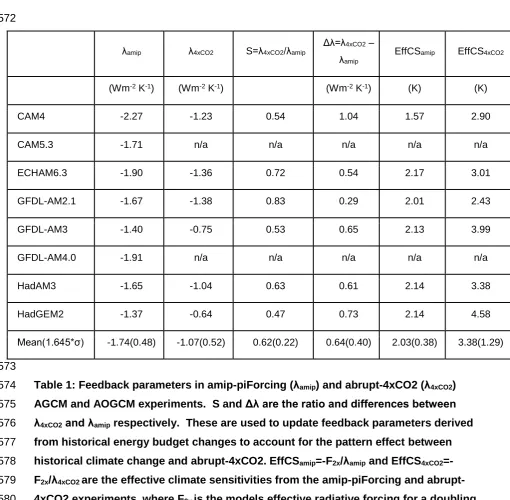
Mean(1.645* ) -1.74(0.48) -1.07(0.52) 0.62(0.22) 0.64(0.40) 2.03(0.38) 3.38(1.29)

[image:19.595.38.549.101.601.2]

573

Table 1: Feedback parameters in amip-piForcing ( amip) and abrupt-4xCO2 ( 4xCO2)

574

AGCM and AOGCM experiments. S and are the ratio and differences between

575

4xCO2and amip respectively. These are used to update feedback parameters derived

576

from historical energy budget changes to account for the pattern effect between

577

historical climate change and abrupt-4xCO2. EffCSamip=-F2x/ amip and EffCS4xCO2

=-578

F2x/ 4xCO2 are the effective climate sensitivities from the amip-piForcing and

abrupt-579

4xCO2 experiments, where F2x is the models effective radiative forcing for a doubling

580

of CO2 (calculated from the abrupt-4xCO2 experiments using a linear regression

581

technique as per Andrews et al., 2012).

(20)

[image:20.595.62.521.100.585.2]

Figures

583

584

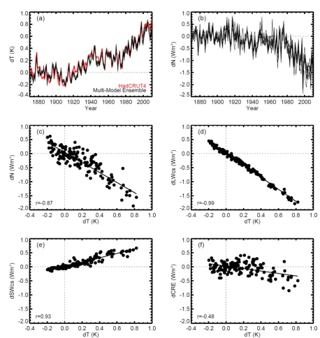
Figure 1: (a) Comparison of historical near-surface-air-temperature change (dT)

585

simulated by the AGCMs in amip-piForcing (individual black lines) against observed

586

(HadCRUT4) variations (red). (b) Timeseries of the change in net TOA radiative flux

587

(dN) in the individual AGCM experiments. (c - f) The relationship and correlation

588

coefficent (r) between the multi-model ensemble-mean (c) dN, (d) LW clear-sky

589

radiative flux change, dLWcs, (e) SW clear-sky radiative flux change, dSWcs, and (f)

590

cloud radiative effect change, dCRE, against dT. All points are global-annual-means

591

covering the historical period (1871-2010) and fluxes are positive downwards.

592

Changes are relative to an 1871-1900 baseline.

(21)

[image:21.595.76.519.71.561.2]

594

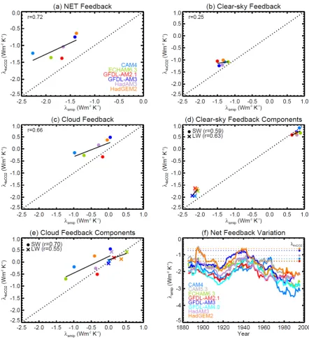
Figure 2: Relationship between the feedback parameter evaluated by regression of dN

595

against dT over the historical period (1871-2010) in amip-piForcing ( amip) and 150yrs

596

of abrupt-4xCO2 ( 4xCO2) for (a) NET radiative feedback, (b) Clear-sky component, (c)

597

CRE component, (d) LW and SW clear-sky components, (e) LW and SW CRE

598

components. (f) Timeseries of amip for individual AGCMs evaluated by linear

599

regression of dN against dT in a sliding 30 year window in the amip-piForcing

600

experiments, the year represents the centre of the window. Coloured circles in (f) with

601

horizontal lines show the feedback parameter values from abrupt-4xCO2.

(22)

[image:22.595.58.514.81.470.2]

603

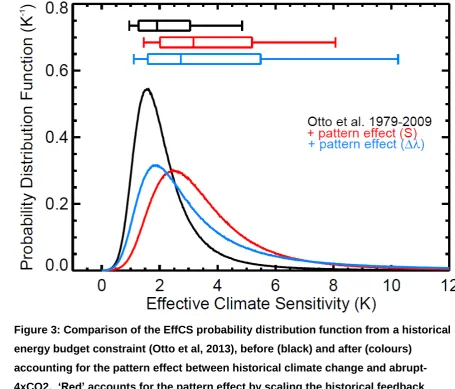
Figure 3: Comparison of the EffCS probability distribution function from a historical

604

energy budget constraint (Otto et al, 2013), before (black) and after (colours)

605

accounting for the pattern effect between historical climate change and

abrupt-606

4xCO2. ‘Red’ accounts for the pattern effect by scaling the historical feedback

607

parameter hist by the ratio (S= 4xCO2/ amip) of the feedbacks found in the

amip-608

piForcing and abrupt-4xCO2simulations. ‘Blue’ accounts for the pattern effect by

609

adding the difference in feedbacks ( = 4xCO2- amip)to hist (see Section 4 and Table 1).

610

Box plots show the 5-95% confidence interval (end bars), the 17-83% confidence

611

interval (box ends) and the median (line in box).