Control of Voltage in Proton Exchange Membrane Fuel Cell Using Model Reference Control Approach

Int. J. Electrochem. Sci., 7 (2012) 6752 - 6761

International Journal of

ELECTROCHEMICAL

SCIENCE

www.electrochemsci.org

Control of Voltage in Proton Exchange Membrane Fuel Cell

Using Model Reference Control Approach

Hamideh Najafizadegan*, Hassan Zarabadipour

Electrical Engineering Department, Imam Khomeini International University, Qazvin, Iran *

E-mail: [email protected]

Received: 9 June 2012 / Accepted: 12 July 2012 / Published: 1 August 2012

The Proton Exchange Membrane Fuel Cell (PEMFC) is one of the most important power supplies. Maintaining a constant voltage in PEM fuel cells has always attracted the attention of many researchers and many articles have been published on this issue. This paper presents a transfer function model of a PEM fuel cell. Subsequently, Model Reference Control (MRC) strategy is proposed to fix fuel cell voltage in presence of noise and disturbance. The model and the controller are implemented in the MATLAB and SIMULINK environment and results are compared with a PID controller.

Keywords: Model Reference Control, PEM Fuel Cell, Transfer Function Model.

1. INTRODUCTION

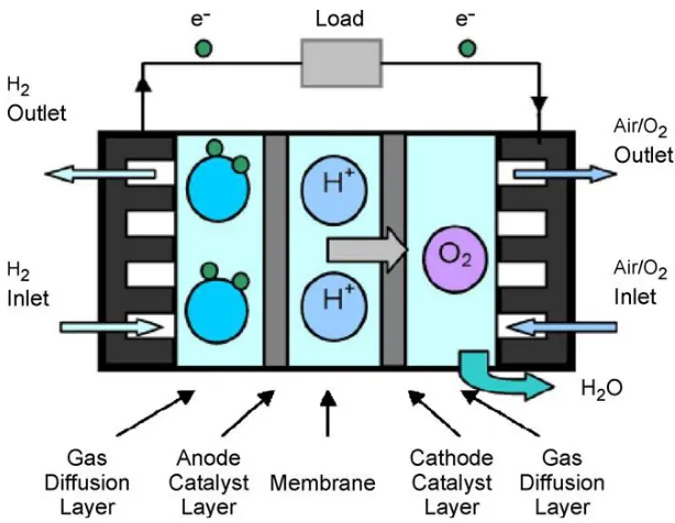
Proton Exchange Membrane fuel cells (PEMFC) are electrochemical energy conversion devices that convert the chemical energy of supplied reactants (hydrogen and oxygen) into electricity. To summarize the operation simply, reactant gases are supplied to both electrodes of the fuel cell via the channels, the gas diffusion layer facilitates even distribution to the catalyst-coated membrane, and the catalyst accelerates the oxidation and reduction of the reactants, which are the primary reactions desired for fuel cell operation (Figure 1).

The H₂ oxidation on the anode side of the membrane releases two electrons, which then traverse the circuit to satisfy the load required of the cell, while the remaining protons (H) travel through the membrane to the cathode side. The O₂ reduction on the cathode side splits the oxygen molecule, which then joins with the electrons completing the circuit and the protons from the membrane to form product water [1].

controlled, is presented. In order to control fuel cell voltage, we use MRC algorithm. The idea of the MRC is based upon the existence of the reference model, specified by the designer, which reflects the desired behaviour of the controlled structure. The controller is designed in such a manner that the output of the controlled structure should track the output of the reference model [2, 3].

Figure 1. Schematic representation of fuel cell electrochemistry

This paper is organized as follows: Section 2 reviews the considered PEMFC’s model. Section 3, explains the Model Reference Control (MRC) algorithm. The results are presented in Section 4 and, finally, conclusions are stated in Section 5.

2. THEORETICAL MODEL OF A PEM FUEL CELL

In order to control fuel cell voltage, first, it is necessary to consider the dynamic model. In recent years, many papers have been written by researchers about dynamic modeling of PEMFC [4]-[7]. Thus in this paper a model that has been previously presented by [8] is used. This model is a theoretical model of a proton exchange membrane (PEM) fuel cell.

In fuel cells, the movement of electrons through the external circuit and protons through the membrane for a single cell generates a voltage difference between the cell terminals. This voltage can be defined by Equation (1), [5], [9].

cell Nernst act ohm conc

where E_Nernst is the cell thermodynamic potential drop. In this model, E_Nernst is calculated from the Nernst equation taking into account temperature changes with respect to reference standard temperature. This voltage can be calculated from the Nernst equation [5] given as









 

1

ln ln ,

2 2 2 2

Nernst ref H O

G S RT

E T T P P

F F F

   

    _  _

  (2)

where G is the change in the free Gibbs energy of the reaction (J mol/ ), F is the constant of Faraday (96485.309 C mol/ ), S is the change of entropy of the reaction (J mol/ ),R is the universal constant of the gases (83.143 J mol K/ / ) and P_H2 and P_O2 are the partial pressures of hydrogen and oxygen (atm), respectively. Variables T and T_ref denote the cell operating temperature and the reference temperature (K ), respectively.

The second term of Equation (1), V_act is the activation overpotential which can be calculated by

 

 





act o FC

V     T T C T I (3)

where IFC is the static current passing through the cell and    1, 2, 3, 4 represent the experimental

coefficients depending on each type of cell. Oxygen concentration (CO2) in the interface between the

cathode and the catalyst ( 3

/

mol cm ) is given by [10]

2

2 ,

5.08 6 exp( 498 / )

O O P C e T 

 (4)

In practice, the third addend of Equation (3) has a very low value as compared with the rest of addends. Therefore, it can be rejected.

The third term of Equation (1) is the ohmic voltage drop, V_ohm. This term represents the voltage drop due to resistance to the transfer of electrons through the electrodes and to the transfer of protons through the membrane. The expression of the voltage drop due to ohmic losses is





ohm FC M C

V I R R (5)

where R_C represents the resistivity to the transfer of electrons through the electrodes. It is usually considered with a constant value.

The equivalent resistance of the membrane (RM) is calculated as

, M M l R A 

 (6)







 















2 2.5

181.6 1 0.03 / 0.062 / 303 /

,

0.634 3 / exp 4.18 303 /

FC FC

M

FC

I A T I A

I A T T

   _{ }         

  (7)

The parameter  is an adjustable parameter with a maximum value of 23. This parameter depends on the membrane fabrication process and is a function of the relative humidity and the stoichiometric rate of the gas in the anode. Under ideal humidity conditions (100%), this parameter may have a value ranging from 14 to 20.

The last addend of Equation (1) is the term corresponding to concentration voltage drop, V_conc. This drop is mainly due to the reactive concentration excess near the catalyst surfaces. This voltage drop can be known from

max

ln 1 ,

conc J V B J     _  _

  (8)

where B is a parameter that depends on the type of cell and J represents the current density passing through the cell at each moment (A cm/ 2) and is defined as

,

FC

I J

A

 (9)

The transfer function of fuel cell is as (11) which was obtained from [8]. This transfer function relates the voltage between the fuel cell terminals (v_FC) to the current provided by the fuel cell (i_FC), round a generic operating point following expression

 

_{ }

 





,

FC

FC FC FC FC FC

FC

v s

G s C sI A B D

i s



    (10)

Being scalar matrixes, the fuel cell transfer function is simplified in the form

 

_



_



FC

FC

C B D s A

G s

s A

 



 (11)

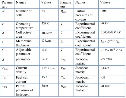
The Values resulting from each of the parameters are given in Table 1. Jacobean matrixes of PEMFC (AFC,BFC,CFC and DFC) are obtained from [8].

Under normal operating conditions, a single cell produces approximately1.2V . For use in energy generating systems, where a relatively high power is required, several cells are connected in series, forming a stack that can supply electrical power of the order of some kilowatts.

For a stack formed by N cells, the voltage between its terminals is obtained from:

,

FC cell

3. MODEL REFERENCE CONTROL (MRC)

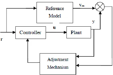
In Model Reference Control (MRC), the desired plant behavior is described by a reference model which is driven by a reference input. The control law is then developed so that the closed-loop plant has a response equal to response of reference model. This response matching guarantees that the plant will behave like the reference model for any reference input signal (Figure 2).

3.1. The MIT Rul

Table 1. Values used for parameters and jacobian matrixes of pemfc

Parame ters

Names Values Parame

ters

Names Values

N Number of

cells

33 PO2 Partial

pressures of oxygen

1atm

T Operating

temperature

338 K _{1 Experimental}

coefficient

0.8V



A Cell active

area

2

40.6 cm 2 Experimental

coefficient

0.0036008V /K

l Membrane

thickness

178 m _{3 Experimental}

coefficient

5

7.6 10  V /K

 _Adjustable

parameter

19.5 4 Experimental

coefficient

4

1.35 10 V /K

 

B parameter 0.1V AFC Jacobean

matrix 29.7299  max J Current density 2

1.42A/ cm BFC Jacobean

matrix

0.1422

FC

I Fuel cell

current

45A C_FC Jacobean

matrix 33  2 H P Partial pressures of hydrogen

3atm D_FC Jacobean

matrix

0.1887



This rule was developed in Massachusetts Institute of Technology and is used to apply the MRC approach to any practical system. In this rule the cost function or loss function is defined as [12]

 

, 2

J   e (13)

that the loss function is minimized. For this object it is reasonable to change the parameter in the direction of the negative gradient of J , that is,

,

d J e

e dt

 _{ }

 

 

   

  (14)

The partial derivative term  e/ , is called the sensitivity derivative of the system. This shows how the error is dependent on the adjustable parameter . There are many alternatives to choose the loss function J , like it can be taken as mode of error also. Similarly d/dt can also have different relations for different applications.

Figure 2. Model Reference Controller

Let the actual system is described by

 

y

kG s

u  (15)

where G s

 

 

 

0 ,

m

m

y

k G s G s

r   (16)

where r is the reference input, y_m is the reference output and k₀ is known. The controller output or manipulated variable is chosen as

,

u r (17)

The output error is defined as

 

 

m

Here the object is to compare the actual output (y ) and the reference output (y_m) and by

applying Model Reference Control Scheme the overall output will be improved. The sensitivity derivative of the system is as

 

0

,

m

e k

kG s r y

k



 _{ }

 (19)

The update rule for the controller parameters using MIT rule is described by

0

,

m m

d k

y e y e

dt k

 _{ }

    (20)

4. SIMULATION RESULTS

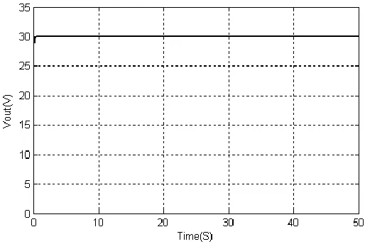
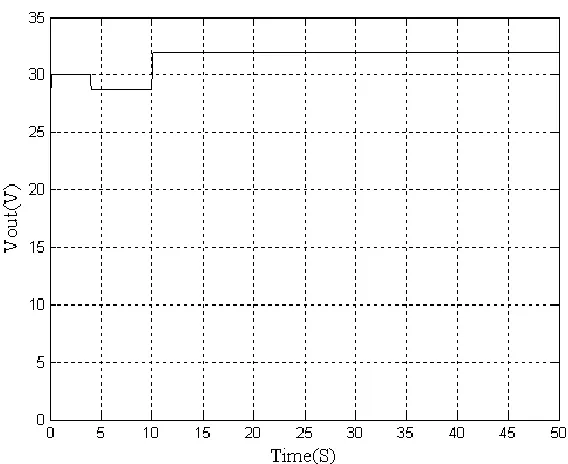
In this section, the ability of proposed controller is proved for set the output voltage at 30V and the capability of proposed controller is compared with PID controller. In simulation, first a white noise is added to input that is fuel cell current (I_FC 45A). Then a perturbation is caused in the input variable that is fuel cell current (I_FC ). In simulation, a testing current 45.88A is loaded at the beginning and suddenly reduced to 44A. Then, it raised 5A .

Figures 3-8 show the simulation results. As it can be seen, the model reference controller able to maintain voltage at 30V (Figures 3, 6) while the PID controller is unable to maintain a constant voltage (Figures 4, 7). The output voltage without controller is shown in Figures 5, 8.

Figure 4. Output voltage with PID controller in presence of noise

Figure 5. Output voltage without controller in presence of noise

Figure 7. Output voltage with PID controller in presence of disturbance

Figure 8. Output voltage without controller in presence of disturbance

5.CONCLUSION

References

1. B.A. McCaina , A.G. Stefanopouloua, I.V. Kolmanovsky, Chemical Engineering Science 63 (2008) 4418 – 4432.

2. P.N. Paraskevopulos, New Jersey: Prentice Hall; 1996.

3. H. Kaufman, I. Barkana, K. Sobel, Second ed. New York: Springer-Verlag 1998.

4. C. Wang, H. Nehrir, R. Shaw Steven, IEEE Trans Energy Converse 20 (2005) 442-451. 5. J.E. Larminie and A, Chichester, U.K:Wiley, (2000) 308-308.

6. K. Kirubakaran, S. Jain, R.K. Nema, Int. J. Recent Trends in Engineering, 3 (2009).

7. J.T.Pukrushpan, A.G.Stefanopoulou, H.Peng, Control of Fuel Cell Power Systems, Springer, New York, 2004.

8. J.M. Andujar, F. Segura, M.J. Vasallo, Renewable Energy 33 (2008) 813–826.

9. J. Amphlett, R. Mann, B. Peppley, P. Roberge, A. Rodrigues, J Power Sources 61 (1996) 183–188. 10.J. Amphlett, R. Baumert, R. Mann, B. Peppley, P. Roberge, J Electrochem Soc 142 (1995) 1-8. 11.J. Corr ˆea, A. Farret Felix, N. Canha Luciane, G. Sim ˜oes Marcelo, IEEE Trans Indust Electron

51 (2004) 1103–1111.

12.Y.D. Landau, Marcel Dekker, New York, 1979.