Int. J. Electrochem. Sci., 7 (2012) 8734 - 8744
International Journal of
ELECTROCHEMICAL
SCIENCE
www.electrochemsci.orgImproved Model Predictive Control for
a
Proton Exchange
Membrane Fuel Cell
Liping Fan 1,*, Jun Zhang 1, Yi Liu 2, Xiaolin Shi 1
1
Shenyang University of Chemical Technology, Shenyang, 110142, China
2
North Heavy Industry Group Co., Ltd, Shenyang, 110141, China
*
E-mail: [email protected]
Received: 23 July 2012 / Accepted: 17 August 2012 / Published: 1 September 2012
Proton exchange membrane fuel cells are promising energy sources. Because of their time-change, uncertainty, strong-coupling and nonlinear characteristics, proton exchange membrane fuel cells present complex control challenges. Based on mathematical modelling and numerical simulations, two improved model predictive controllers which use Laguerre function and exponential data weighting are proposed for the proton exchange membrane fuel cell to realize constant power output. Simulation results show that the proposed model predictive controllers can give good control effects.
Keywords: Fuel cell; model predictive control; laguerre function; exponential data weighting
1. INTRODUCTION
Fuel cells are promising energy sources that produce electrical currents with almost null pollutant emissions. In the recent years there was an increasing interest in fuel cell technology. Although they were invented more than a century ago, they have received much attention in the last decade as good candidates for clean electricity generation both in stationary and automotive applications. Proton exchange membrane fuel cell (PEMFC) is one of the most interesting fuel cells types due to its low operating temperature, high efficiency and low electrolyte corrosion [1-3]. They are acknowledged as most valuable new alternative energy sources.
[4-5]. In many applications, keeping a fuel cell in a state of constant power output is necessary. So, maintaining a fuel cell system in correct operating conditions is necessary and it requires good control system. Model predictive control (MPC) is an optimization strategy for the control of constrained dynamic systems [6-7]. MPC uses multi-step prediction, rolling optimization and feedback correction control strategies [8], so it can not only give a good control effect and strong robustness, but also have an advantage of less demand on the accuracy of the model. It is an effective method to solve complex industrial process control [9-10]. However, some problems still need to be solved when using MPC in a real system. It is well know that the traditional approach of expanding the future control signal uses the forward shift operator to obtain the linear-in-the-parameters relation for predicted output in designing a MPC. In the case of rapid sampling, complicated process dynamics or high demands on closed-loop performance, satisfactory approximation of the control signal requires a very large number of forward shift operators, and leads to poorly numerically conditioned solutions and heavy computational load when implemented on-line. So, improved strategies are needed to solve these problems.
This paper is organized as follows. The mathematical model for a typical proton exchange membrane fuel cell is described in Section 2. Section 3 presents a brief description of designing improved MPC controllers for PEMFC. Simulation results are presented in section 4 to confirm the effectiveness and the applicability of the proposed method.
2. MATHEMATICAL MODEL OF PEM FUEL CELL
PEM fuel cell electrochemical process starts on the anode side where H2 molecules are brought
by flow plate channels. Anode catalyst divides hydrogen on protons H+ that travel to cathode through membrane and electrons e- that travel to cathode over external electrical circuit. At the cathode hydrogen protons H+ and electrons e- combine with oxygen O2 by use of catalyst, to form water H2O
and heat. Described reactions can be expressed by the following equations [11-14]:
) (Anode 2
2
2
H e
H (1)
(Cathode) 2
2 1
2 2 H e H O
O (2)
The output voltage Vfc of a single cell can be defined as the result of the following expression
con ohmic act
nernst
fc E V V V
V (3)
in which Enernst is the thermodynamic potential of the cell representing its reversible voltage,
2 2
3 -5
nernst fc fc
1 1.229 0.85 10 ( 298.15) 4.31 10 ln( ) ln( )
2
H O
E T T P P
(4)
where PH2 and PO2 (atm) are the hydrogen and oxygen pressures, respectively, and Tfc (K) is the
operating temperature. Vact is the voltage drop due to the activation of the anode and the cathode:
2
3 5 4
act 0.9514 3.12 10 fc 7.4 10 fcln( O ) 1.87 10 fcln( )
V T T C T i (5)
where i (A) is the electrical current, and CO2 is the oxygen concentration. Vohmic is the ohmic
voltage drop associated with the conduction of protons through the solid electrolyte, and electrons through the internal electronic resistance:
) (
ohmic i RM RC
V (6)
where RC () is the contact resistance to electron flow, and RM () is the resistance to proton
transfer through the membrane, which can be described as
2 2.5 fc
M
fc fc
181.6 1 0.03 0.062
303
-303
0.634 3 exp 4.18
M M
l R
A
T
i i
A A
T i
A T
(7)
where ρM(cm) is the membrane specific resistivity, l (cm) is the membrane thickness, A
(cm2) is the membrane active area, and ψ is a specific coefficient for every type of membrane; Vcon
represents the voltage drop resulting from the mass transportation effects, which affects the concentration of the reacting gases and can be described by the following expression:
) 1 ( ln
max con
i i B
V (8)
where B (V) is a constant depending on the type of fuel cell, imax is the maximum electrical
current. The output power of the single fuel cell is
i V
Pfc fc (9)
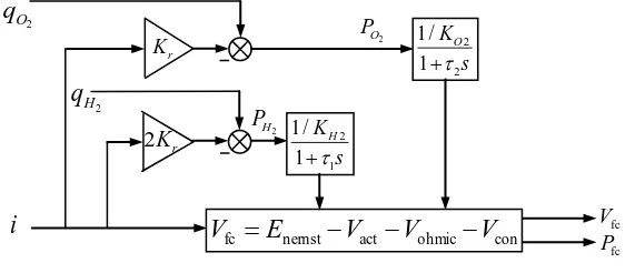
Fig. 1 shows a generallyaccepteddynamic model of the PEM fuel cell, in which qO2 is the
constant, and KO2 is oxygen valve molar constant [15-16]. Based on the above described mathematical
[image:4.596.158.439.159.282.2]model, a Matlab/Simulink simulation model of the PEMFC can be set up [17]. Parameters of the Ballard Mark V fuel cell [18] are used in the simulation model.
Figure 1. PEMFC dynamic model
3. DESIGN OF MPC AND IMPROVED MPC
Constant power sources are needed in some applications. So, keep fuel cells in constant power output state is necessary in such applications. In order to make the PEM fuel cell keep constant power output, MPC with laguerre and exponential data weighting for constant voltage output are designed and compared. The core technique in the design of discrete-time MPC is based on optimizing the future control trajectory, that is the difference of the control signal,u k( ).The traditional approach of expanding the future control signal uses the forward shift operator to obtain the linear-in-the-parameters relation for predicted output in designing a MPC. As a consequence, in the case of rapid sampling, complicated process dynamics or high demands on closed-loop performance, satisfactory approximation of the control signal requires a very large number of forward shift operators, and leads to poorly numerically conditioned solutions and heavy computational load when implemented on-line [19].
Laguerre function is famous for its orthogonality. Its expression is so simple that the computation load could get greatly reduced and it has a good effect on the parameterization presents a parsimonious description of the future control signal, hence reduces the number of parameters required in modelling the control trajectory. What’s more , when the scaling factor is chosen at 0, the laguerre functions are equal to the expression of the traditional control variable, which is to say, Laguerre functions control strategy include the traditional MPC strategy. The z-transforms of the discrete-time laguerre networks can be shown as following [20]
2 2
1/ 1
O K
s
r K
con ohmic act
nernst
fc E V V V
V
2 1
1 / 1
H K
s
2Kr
i
2 H
q
2
O
q
2
H P
2
O P
fc
P
fc
2 1 1 2 12 1 1
2 1 1 1 1 1 1 1 1 1 1 ( ) 1 1 N N a z az
a z a
z
az az
a z a
z az az (10)
where a is the pole of the discrete-time laguerre network and it is the scaling factor, and 0 ≤ a < 1 for stability of the network. Let l ki( )denote the inverse z-transform of i( , )z a , in which i is between 1 and N. This set of discrete-time laguerre functions are expressed in a vector form as
1 2
( ) [ ( ), ( ), N( )]T
L k l k l k l k and the laguerre sequences can be computed using the following state space
model:
( 1) ( )
L k HL k (11)
where
2
2 2 3 3
0 0 0
0 0
0
0
( 1)N N ( 1)N N
a
a
a a
H
a a
a a a
; 2 3 1 1 1 (0)
( 1)N N
a a L a a (12)
and 2
1 a
. At time ki, the control trajectories u k( ), i u k( i1), u k( i2), u k( ik), is regarded as the impulse response of a stable dynamic system. Thus, a set of laguerre functions,
1( ), ( ),2 N( )
l k l k l k are used to capture this dynamic response with a set of laguerre coefficients that will be determined from the design process. More precisely, at an arbitrary future sample instant k
1
( ) ( ) ( )
N
i j i j
j
u k k c k l k
(13)with ki being the initial time of the moving horizon window and k being the future sampling
instant; N is the number of terms used in the expansion and cj, j=1, 2, . . . , N, are the coefficients, and
they are functions of the initial time of the moving horizon window ki. Let [1 2 ]
T N
c c c
and
( i ) ( )T
u k k L k
( 1) ( ) ( )
( ) ( )
m m m m
m m
x k A x k B u k
y k C x k
(14)
Let x km( )
x km( )x km( 1)
, y k( )C x km m( ) , and choosing a new state variable
( ) m( ) ( )T
x k x k y k , then the MPC state space model can be expressed as follows:
( 1) ( )
( )
( 1) 1 ( )
( ) ( ) [ 1]
( )
T
m
m m m m
m m m m
m m
B
x k A O x k
u k C B
y k C A y k
x k
y k O
y k (15)
where Om is a zero matrix. The Eq. (15) can be written as:
( 1) ( ) ( )
( ) ( )
x k Ax k B u k
y k Cx k
(16)
An improved predictive formulation in which u k( ii) is replaced by ( ) T i
L k can be shown
as: 1 1 0 1 1 0 ( ) ( ) ( ) ( ) ( ) ( ) m
m m i T
i i i
i m
m m i T
i i i
i
x k m k A x k A BL i
y k m k CA x k CA BL i
(17)where x k( im ki) and y k( im ki) are the predicted state variables and the predicted output at
ki+m with given current plant information x(ki). Then we get a new expression of the cost function
2 ( )
T T
i
J x k (18)
where 1 ( ( ) ( ) ), P N T L m
m Q m R
1 ( ( ) ), P N m m m QA
RL is a designed matrix; and1 1
0
( ) ( )
m
m i T
i
m A BL i
with TQC C.
To find the minimum of Eq. (18) without constraints, we assume that 1
is existent. Then the optimal solution of the parameter vector η can be obtained by letting the partial derivative of the cost function approach to zero.
It is noted that in the finite prediction horizon, the condition number of the matrix increases as the prediction horizon NP increases. When there is an integrator in the system matrix A, the norms of
increase as the prediction horizon NP increases. Hence, if the prediction horizon NP is large, a
numerical conditioning problem occurs. This numerical problem becomes severe when the plant model itself is unstable, or when the dimension of the matrix A is large. An exponentially weighted moving horizon window can convert the numerically ill-conditioned matrix into a numerically well-conditioned in the presence of a large prediction horizon and could deal with great changes of the plant which originally get serious problems.
Define the sequence of exponentially weighted incremental control as
0 1 2
ˆ [ ( ),i ( i 1), ( i 2), Np ( i )]T
U u k u k u k u k Np
(19)
where 1 is used to scale the eignvalues of matrix A, and the exponentially weighted state
variable is denoted as
1 2 3
ˆ [ ( i 1 i), ( i 2 i), ( i 3 i), Np ( i i)]T
X x k k x k k x k k x k Np k (20)
By using these exponentially weighted variables, the exponentially weighted cost function is expressed in terms of the transformed variables. The result is summarized by the theorem below:
1 0
ˆ Np ˆ( )T ˆ( ) Np ˆ( )T ˆ( )
i i i i i i
j j
J x k j k Qx k j k u k j R u k j
(21)where Q and R are weight matrices, ˆ(x ki j ki) and u kˆ( i j) are governed by the following difference equation:
ˆ( i 1 i) ˆ( i i) ˆ( i )
A B
x k j k x k j k u k j
(22)
In this research, when the plant is running under the traditional MPC, the predictive horizon is 20, the control horizon is 5, and the output weight is a unit matrix. When the plant is running under the MPC with laguerre functions substituting the control variables and under the MPC with exponentially weighted corrected, the two core factors are: a is 0.8 and N is 1.5, the predictive horizon is 48, the weighting QCT*C, and R=0.3; what’s more, is chosen as 1.25 in the MPC with exponentially
weighted corrected control strategy. The sampling time of the three control strategies is 0.1s. The control variables change in the range of [0, 10] when oxygen flow is chosen to adjust and [0, 20] when hydrogen flow is chosen to adjust, and the incremental of control variables ranges from -2 to 2. The output constrains are ignored in this paper. So far, all the parameters are all given.
4. RESULTS AND DISCUSSION
fuel cell system with these various controllers is carried out. Forthepurposeof designing MPC controller, Least Square Technique is used to identify the state space model of PEM fuel cell described in Eq. (14), and the identification solutions of the coefficientmatricesare
0.9226 0.0153 0.0961 0.9992
0.0961; 0.0049
[0 0.0378] 0
m
m
m
m
A
B
C
D
(23)
According to the principle of MPC, the parameter matrices corresponding to Eq. (16) can be derived as
1.9218 0.9233 0.0002 0 0.0002
1 0 0 0 0
,
0 0 0 0 1
1.9218 0.9233 0.0002 1 0.0002
[0 0 0 1], 0
A B
C D
(24)
Three control strategies are designed and compared in this paper, including traditional MPC with reduced horizon control, improved MPC with Laguerre functions and improved MPC with exponential data weighting. Meanwhile, these three controllers are designed for two control schemes respectively, one is control the output power by adjusting the hydrogen flow, and the other is control the output power by adjusting the oxygen flow.
0 5 10 15 20 25 30 35
0 0.1 0.2 0.3 0.4 0.5 0.6 0.7
t/s
P
fc
/w
RHC lag
0 5 10 15 20 25 30 35
0 1 2 3 4 5 6
t/s
q
O
2
/(
k
m
o
l/
s
)
[image:8.596.87.512.506.676.2]RHC lag
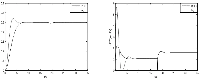
Figure 2. Traditional MPC and Laguerre based MPC with oxygen flow as the control variable
The main parameters of the fuel cell model used in these operations are B=0.016V, A=50.6cm2, Tfc=343k, Rc=0.0003, l=0.0178cm, ψ=23.
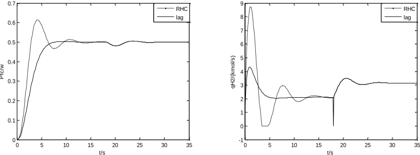
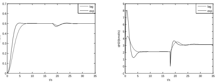
Figure 2 to Figure 5 report the simulation operation results under these dissimilar control schemes. In these figures, RHC stands for the traditional MPC strategy, lag stands for improved strategy with Laguerre functions and exp stands for the improved strategy with exponential data weighting. Multiple comparisons are shown in these figures.
It can be seen from these figures that the control effects are getting more and more well through step-by-step improvement schemes. The traditional MPC can make the system reach an elementary control objective roughly, but it cause big overshoot and long regulating time. The improved MPC with Laguerre functions or exponential data weighting can give better control effects. Both oxygen flow and hydrogen flow can be used as operatingvariable, and the control effects are similar, but the tracking time caused by adjusting oxygen flow is a bit shorter than that of adjusting hydrogen flow. When load disturbance occur in the system, the improved MPC can make the system return the given steady state rapidly after a short fluctuation. Analyzing by synthesis of steady state error, rapidity and overshoot, the improved MPC with exponential data weighting can give more desirable control effect than the other two control schemes, and the output power can keep in a given value well.
0 5 10 15 20 25 30 35 0
0.5 1 1.5 2 2.5 3 3.5 4 4.5
t/s
q
O
2
/(
k
m
o
l/
s
)
lag exp
Figure 3. Improved MPC based on Laguerre function and exponential data weighting adjusting oxygen flow
0 5 10 15 20 25 30 35 0
0.1 0.2 0.3 0.4 0.5 0.6 0.7
t/s
P
fc
/w
RHC lag
0 5 10 15 20 25 30 35 -1
0 1 2 3 4 5 6 7 8 9
t/s
q
H
2
/(
k
m
o
l/
s
)
[image:9.596.93.514.353.512.2]RHC lag
Figure 4. Traditional MPC and Laguerre based MPC with hydrogen flow as the control variable
0 5 10 15 20 25 30 35 0
0.1 0.2 0.3 0.4 0.5 0.6 0.7
t/s
P
fc
/w
[image:9.596.98.524.580.737.2]
0 5 10 15 20 25 30 35 0
0.1 0.2 0.3 0.4 0.5 0.6 0.7
t/s
P
fc
/w
lag exp
0 5 10 15 20 25 30 35 -1
0 1 2 3 4 5 6 7 8 9
t/s
q
H
2
/(
k
m
o
l/
s
)
lag exp
Figure 5. Improved MPC based on Laguerre function and exponential data weighting adjusting hydrogen flow
By comparing the results with those results published by other authors [13, 16, 21], it also can be seen that the method presented in this paper can realize outputting a constant power while the other references focused on keeping a constant output voltage. Further, compared with the former method in the same situation of controlling constant power [22], the method proposed in this paper has better control precision and adaptability.
5. CONCLUSIONS
Fuel cells which are required to output constant powers need good power control systems. By using improved MPC controller, the PEM fuel cell can not only have fast response characteristic, but also have good steady-state behavior and strong robustness. The suitable model predictive control scheme can get satisfactory results in tracking a given power and make the fuel cell output a required constant power.
ACKNOWLEDGEMENTS
This work was supported by the National Natural Science Foundation of China under Grant 61143007, and the National Key Technology Research and Development Program of China under Grant 2012BAF09B01.
References
1. S. Das and N. Mangwani, J. Sci. Ind. Res. India., 69 (2010) 727. 2. B. Logan, Appl. Microbiol. Biotechnol., 85 (2010) 1665.
3. J. Pukrushpan, A. Stefanopoulou and H. Peng, IEEE Contr. Syst. Mag., 24 (2004) 30. 4. C. Kunusch, P. Puleston, M. Mayosky and J. Riera, IEEE T. Contr. Syst. T., 17 (2009) 167. 5. S. Kaytakoglu and L. Akyalm,Int. J. Hydrogen. Energ., 32 (2007) 4418.
6. L. Riascos and D. Pereira, ABCM Sym. S. Mech., 4 (2010) 137.
[image:10.596.101.528.76.239.2]
8. L. Domınguez and E. Pistikopoulos, Ind. Eng. Chem. Res., 2 (2011) 609. 9. K. Holkar and L. Waghmare, Int. J. Control. Autom., 3 (2010) 47. 10. S. Qin and T. Badgwell, Control Eng. Pract., 11 (2003) 733. 11. B. Carnes and N. Djilal, J. Power Source, 144 (2005) 83. 12. M. Moreira and G. Silva. Renew. Energ., 34 (2009) 1734.
13. A. Rezazadeh, M. Sedighizadeh and M. Karimi, Int. J. Comput. Electr. Eng., 2 (2010) 81. 14. M. E. Youssef, K. E. NAdi, M. H. Khalil, Int. J. Electrochem. Sci., 5 (2010) 267.
15. K. Mammar and A. Chaker, Int. J. Elec. Eng., 60 (2009) 328.
16. A. Rezazadeh, A. Askarzadeh and M. Sedighizadeh, Int. J. Electrochem. Sci., 6 (2011) 3105. 17. L. Fan, App. Mech. Mat., 121 (2012) 2887.
18. J. Correa, F. Farret, L. Canha and M. Simoes, IEEE T. Ind. Electron., 51 (2004) 1103. 19. L. Wang, J. Process. Contr., 14 (2004) 133.
20. S. Patwardhan, S. Manuja, S. Narasimhan and S. Shah, J. Process. Contr., 16 (2006) 157. 21. H. Najafizadegan and H. Zarabadipour, Int. J. Electrochem. Sci., 7 (2012) 6752 – 6761. 22. L. Fan and Y. Liu, Prz Elektrotechniczn, 88 (2012) 72-75.