Dissolved in Ionic Liquids.
White Rose Research Online URL for this paper: http://eprints.whiterose.ac.uk/151242/
Version: Accepted Version
Book Section:
Ezzawam, WM and Ries, ME (2019) Chapter 3: Diffusion and Relaxometry to Study Carbohydrates Dissolved in Ionic Liquids. In: Zhang, R, Miyoshi, T and Sun, P, (eds.) NMR Methods for Characterization of Synthetic and Natural Polymers. Royal Society of
Chemistry , Croydon, UK , pp. 36-62. ISBN 978-1-78801-400-7 https://doi.org/10.1039/9781788016483-00036
© 2019, The Royal Society of Chemistry. This is an author produced version of a book chapter published in NMR Methods for Characterization of Synthetic and Natural Polymers. Uploaded in accordance with the publisher's self-archiving policy.
[email protected] https://eprints.whiterose.ac.uk/
Reuse
Items deposited in White Rose Research Online are protected by copyright, with all rights reserved unless indicated otherwise. They may be downloaded and/or printed for private study, or other acts as permitted by national copyright laws. The publisher or other rights holders may allow further reproduction and re-use of the full text version. This is indicated by the licence information on the White Rose Research Online record for the item.
Takedown
If you consider content in White Rose Research Online to be in breach of UK law, please notify us by
CHAPTER 4
Diffusion and Relaxometry to Study Carbohydrates Dissolved in Ionic Liquids
W.M. Ezzawam a,b and M. E. Ries a*
a University of Leeds, School of Physics and Astronomy, Woodhouse Lane, Leeds, LS2 9JT, United Kingdom b Tripoli University, Department of Physics, PO Box 13275, Tripoli, Libya
*Corresponding contributor. E-mail: [email protected]
NB Books in the Issues in Environmental Science and Technology series do not have chapter
numbers.
Section headings should follow the numbering: 1 Main section heading; 1.1 Sub section heading;
1.1.1 Lower sub section heading.
Abstract
4.1 Introduction
Nuclear Magnetic Resonance (NMR) is employed to determine both molecular structure and dynamics in a wide range of scientific disciplines. NMR can study the chemical and physical properties of molecules in solution and solid state; it can determine crystallinity, solubility of solution1, phase changes, conformational exchange, diffusion and rotational motion2. This is all achieved by exploiting the spin / magnetic properties of certain NMR active nuclei. If these nuclei are within a liquid then they will move randomly about through a process of diffusion, known as Brownian motion. If this liquid is within an applied magnetic field that has a spatial dependence, a field gradient, then this will cause the nuclear processional frequencies to vary with time. It is this phenomenon that enables NMR to quantify the diffusion of the nuclei, through the detection of the resultant time dependence of the NMR signal that itself is a result of the time dependence of these processional frequencies 3. The self -diffusion coefficient, D, can be defined by the position r(t) of the molecule or ion in the medium at a given time t, through the classic Einstein equation 4
(4.1)
The value of the diffusion coefficient depends on the shape of the ions/molecules, their size, and the
viscosity of the solution they are within5, 6. The correlation between translational diffusion of ions/molecules and the thermal energy in a viscous medium is given by the classic Stokes Einstein relationship4.
(4.2)
where k is the Boltzmann constant, T is the temperature, is the viscosity of the solution and is the effective Stokes radius of the ion or molecule. The constant ƒ is a correction term, also known as the micro-viscosity
pre-factor. It is equal to 1 when the diffusing particle is much larger than the size of the surrounding molecules that make up the medium through which it diffuses 7. It can also be less than one if the particle is similar in size to the surrounding molecules that comprise the viscous medium 6, 8. According to McLaughlin, the value 4 should be used instead of the 6 in the Stokes-Einstein equation, when the size of the diffusing particles is the same as that of the surrounding molecules, which in effect makes f= 2/3 in the above equation6, 9. At room temperature, the values of diffusion coefficient are typically in the range between and
for molecules in liquids 10, 11. The hydrodynamic radius, of particles can be determined from the diffusion coefficient and the ratio of the temperature to viscosity through this Stokes-Einstein equation. The
effective hydrodynamic radius, , of a molecule in a solution can also be estimated through the average
volume that it occupies via the following equation6, 12:
where is the Avogadro number, is density of the medium, is the molar mass and is the molar
volume of the diffusing particles i. Equation 4.3 is used in many studies and has been shown to give reasonable approximate values for the effective radii of ions 6, 11-13.
In a system of interacting NMR active nuclei the relaxation times T1 and T2 can be related to a rotational correlation time, . These relaxation times and this correlation time depend on temperature; two regimes
can be identified by comparing the correlation time to the Larmor precessional frequency of the nuclei, . 1) Liquid regime, found at a high-temperature limit when relaxation times T1 and T2 are approximately equal, here both relaxation times increase as temperature increase, and rot < < 1. 2) Solid regime, found at low temperature and T1 >> T2, here T1 rises with decrease in temperature, while T2 reduces and rot >> 1. The cross over from one regime to the other occurs at a minimum in T1 when rot = 0.62 6, 14, 15.
According to Bloembergen-Purcell-Pound (BPP) theory, in the liquid regime, the relaxation times T1 and T2
can be determined for an isolated spin pair, consisting of two protons separated by a distance , through,
(4.4)
where A is a constant defined as follows:
A ħ (4.5)
where is the gyromagnetic ratio of protons, ħ is the reduced Planck constant, and is the permeability of
free space 14, 15.
The rotational correlation time, can be related to the size of the rotating molecule through the
Debye-Einstein equation for spherical molecules, as:
(4.6)
where is the zero shear rate viscosity. The above equations 4.4, 4.5 and 4.6 can be combined to give a relationship between relaxation times, viscosity and hydrodynamic radius, as:
(4.7)
Ionic liquids (ILs) are organic salts that have a melting point below 100°C, with some being liquids even below room temperature 16, 17. ILs can be formed from numerous different anions combined with many
different cations 18, 19. The most common cations used are imidazolium, pyridinium, ammonium and
phosphonium derivatives 20. The one most frequently used for biomass processing, including cellulose, is
imidazolium21. Ionic liquids have been employed in many fields, such as solvents, in catalysis, separation
technology and electrically conducting fluids 22, 23. In 1934, Graenacher proposed the use of molten
N-methylpyridinium chloride as a solvent to dissolve cellulose, and observed that this salt has a relatively low melting point at just 118°C 24. Ionic liquids have been employed for dissolution, homogeneous derivatization
and biomass processing. Swatloski originally reported on 1-butyl-3-methylimidazolium chloride [BMIM] [Cl], being technically the first use of an ionic liquid in the field of cellulose technology 25, 26. The most
important reasons to select ILs to process biomass are their ‘‘green’’ credentials (low vapour pressure), potential variety (‘‘designer’’ solvents), as well as the advanced understanding of the solvents’ properties that have developed. Moreover, the use of ILs will allow an increase in solution efficiency and reduction of undesirable solvents, coupled with control and flexibility in the processing methodology 27-29.
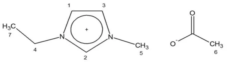
Over the last two decades, the ionic liquid 1-ethyl-3-methylimidazolium acetate [C2mim] [OAc] has received
much attention as an excellent solvent to dissolve polymers such as cellulose and molecules such as carbon dioxide 22, 30, 31. [C2mim] [OAc] has many desirable properties, such as a lower melting point, negligible
vapour pressure and relatively low viscosity, compared with other ILs, in addition it has good thermal stability
32, 33. Therefore, [C2mim] [OAc] is utilized in this work as the solvent to dissolve a variety of carbohydrates,
such as glucose, cellobiose and xylan. The chemical structure of the IL [C2mim] [OAc] solvent is shown in
Figure 4.1. This solvent consists of the imidazolium cation [C2mim] and the acetate, anion [OAc] 20, 33.
[Figure 4.1 near here]
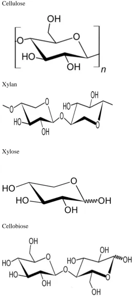
made from elements: hydrogen, oxygen, and carbon35. Here, the structure of four carbohydrates so far described are shown in Figure 4.2.
Cellulose is the world’s most abundant naturally occurring biopolymer, found in plants, bacteria and fungi and is predicted to become the largest source of renewable materials 36, 37. In 1838, the first research on cellulose was carried out by Anselme 38. Cellulose has numerous significant applications in the fibres, paper and paint industries. It has a hydrogen-bonded supramolecular structure, containing D-anhydroglucopyranose units connected by (1 4) glyosidic bonds 39, 40. Hydrogen bonds form between the hydroxyl group of neighbouring chains and give toughness and strength to the cellulose structure 41. Cellulose is insoluble in most organic solvents and water. Therefore, there has been significant effort to find ways to process cellulose using new solvents and reagents42, dating back to the viscose method that uses carbon disulphide 43. The viscose process was developed by scientists Charles Frederick Cross and Edward John Bevan. In 1892, they
obtained British Patent no. 8,700 for ‘‘Improvements in Dissolving Cellulose and Allied Compounds’’ 44.
After cellulose xylan is the second most abundant biopolymer, on earth 45. Xylan is found in the cell walls of plants and comes in a wide range of structures, where this diversity in structures is correlated with their
functions in the plants they are found. It is a polysaccharide and consists predominantly of (1 4) – linked xylose residues 46. The differences in the xylan backbone structure depends on the botanical source. The composition of the xylan backbone commonly contains a galactose, xylose, arabinose and mannose, as well as an esterase group (acetyl and ferulic acid). Like cellulose, xylan is insoluble in water 46. Recent studies are interested in employing xylan in numerous applications, such as paper, food industry, biofuel, as well as in pharmaceutical as a prodrug. Xylan ester have been employed as a carrier drug and also sulphate derivatives to use as antiviral drugs 47, 48. Xylose is a monosaccharide and can be derived from hemicellulose, such as xylan 21. Xylose has a variety of industrial applications such as in pharmaceutical and food production.
Cellobiose, which will be investigate here, is a disaccharide and consists of two D glucopyranose units connected by a (1 4) glyosidic bond 49, 50.
4.2 Experimental Methods
A Bruker Avance II (400MHz) spectrometer with diffusion probe (Diff 50) was used for the diffusion measurements. The measurement of relaxation times T1 and T2 were performed on a 20 MHz “low” field
Maran Benchtop NMR spectrometer.
4.2.1 NMR Diffusion
Diffusion was measured using the method of NMR stimulated echo pulse sequence with bipolar gradients 51, 52, which is produced by a combination of magnetic field gradients and radiofrequency pulses (PFGSE) 53, 54.
Bipolar gradients, g is used for dephasing and rephasing the magnetization positions during the time , and
is the pulse duration of the joint pair of bipolar pulses.54. Experimentally, attenuation of the signal of the intensity of ions in PFGSE is provided by equation 4.8 55, 56.
(4.8)
where and are a diffusion coefficient and the measured signal intensity of ions respectively. is an
initial signal intensity, the time between bipolar gradients, g the gradient strength, and is a period
separating the starting of each pulse pair. The parameters used were 60ms, 2-5ms, g was incremented up
to 20 Tm-1 (gradient field strength was confirmed using water at 20 °C),57 and was kept constant at 2ms 6, 57-59.
4.2.2 NMR Relaxometry
The inversion recovery method is the pulse sequence 180° - -90° and is utilised to measure the relaxation
time T1. After the initial 180° pulse the net sample magnetisation M points along the negative Z-direction and then during M relaxes until it eventually () returns to the original and equilibrium position, pointing
parallel to the positive Z-direction 60, 61. This sequence is repeated for various values and as a function
of is recorded. This function is then fitted to a single relaxation time expression given by:
The pulse sequences for measuring spin-spin relaxation time, T2, was developed by Carr and Purcell in 1954 3. Experimentally, T2 is measured by ‘‘90 x- -(180 x- -measure- -)n’’, which is known as Carr Purcell
Meiboom Gill (CPMG) sequence 3, 61. Experimentally, the relaxation time is approximately exponential and is governed by Equation 4.10. In the transverse relaxation measurement, the magnetization is kept within the XY plane61. The value of magnetisation in the y-direction can be calculated by the equation:
= (4.10)
where My is magnetisation in transverse plane at the echo time . The pulse sequence is employed to eliminate the effects of field inhomogeneities on the measured relaxation time 3, 8, 58, 62.
4.2.3 Viscosity
All rheological measurements were carried out for all carbohydrates solutions using a dynamic stress-controlled rheometer (Kinexus Ultra, from Malvern) equipped with a cone-plate geometry (4°- 40 mm) and a temperature control system, using software called rSpace. A thin film of low-viscosity silicone oil was added around the edges of the plates to prevent moisture-contamination during the viscosity measurements. The Cross – Viscosity Equation has been used to extrapolate to the zero shear rate viscosity, 63. Steady-state
measurements were recorded for temperature between 20 °C to 60 °C inclusive in 10 °C steps, before the experiment was run.
4.2.4 Materials
The ionic liquid 1-ethyl-3-methylimidazolium acetate [C2mim] [OAc] solvent was purchased from
Sigma-Aldrich (purity ≥ 97%, highest obtainable). D-xylose and cellulose powders were obtained from Sigma Aldrich with a purity of 99% for NMR and viscosity measurements. Xylan was extracted from pulping of
4.2.5 Sample Preparation
D-xylose and xylan were dried in vacuum at 50°C for 24h before use. D-xylose and xylan were individually dissolved in [C2mim OAc] solvent to prepare two sets of five samples with different weight fraction (weight fraction: 1%, 3%, 5%, 10% and 15%). Carboyhdrate solutions were stirred under nitrogen gas in an MBraun Lab Master 130 Atmospheric chamber preserved at a dew point between -70 and -40 . The NMR tubes of samples were sealed to prevent contamination with water from the atmosphere within the chamber. Low concentrations of xylose took 48h to dissolve in [C2mim] [OAc] while high concentrations (5%, 10% and 15%) approximately 1 week, these samples were prepared without heat. All carbohydrates solutions were placed in the NMR tubes with depths less than 1 cm to reduce convection currents on heating in the NMR machine. By doing this, we followed the guidance set out by Annat et al 64.
4.3 Results and Discussion
4.3.1 Xylose Results
4.3.1.1 NMR Diffusion
¹HNMR spectroscopy, diffusion, and low field relaxometry (20MHz), across the temperatures range (20 °C to 60 °C), were used to examine the influence of D-xylose on the ions of the IL [C2mim] [OAc]. The ¹H NMR spectrum displays seven peaks, each peak corresponds to a chemically distinct proton within the ionic liquid molecule, see Figure 4.1 33. During measurements of NMR diffusion, it was found that the diffusion coefficients of all cations resonances were approximately equal. The diffusion data of xylose will be compared to cellobiose data, which is taken from Ries et al. 49, to understand the influence of carbohydrate structure, in particular the number of available OH groups, has on that the ions. An Arrhenius type equation was used to
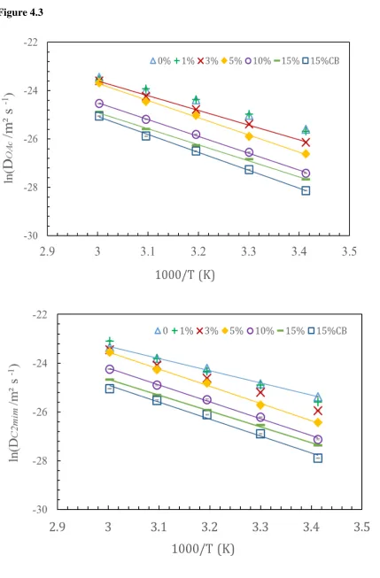
model the temperature dependence of the self-diffusion coefficients of the ions at all the xylose and xylan weight fractions %,
where EA is the translational activation energy for the ions, R is the universal gas constant, T is temperature, and is the zero activation energy limiting value (sometimes known as the high temperature limiting value) of the diffusion coefficients for the ions 49.
In Figure 4.3 (a, b) the solid lines are the Arrhenius fits. The mobility of anions and cations decrease with an increase in xylose weight fraction. The values of diffusion coefficients increase with increase in temperature,
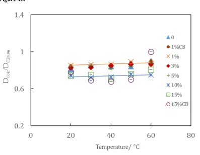
as expected. Figure 4.4 presents the ratio of diffusion coefficients of anions to cations as a function of temperature for xylose and cellobiose49. The ratio of diffusion coefficients of the anion to the cations for all xylose and 1% and 15% cellobiose concentrations, for comparison, were calculated from the data which is presented in Figure 4.3 As the temperature increased the ratio of anion [OAc] to cation [C2mim] diffusivities remained constant, with only a slight dependence on the xylose weight fraction. The 1% and 15% cellobiose data display a similar temperature and concentration dependences. This suggests that both carbohydrates have a similar dissolving mechanism, which thus affects the translational motion of the ions similarly. Cellobiose and xylose have the same number of OH groups per molecule, 4, and this number has been shown to be the key factor in influencing the diffusion of the surrounding ions49. The ratio of anion [OAc] diffusion coefficients to that of cation [C2mim] is less than 1. This is known as ‘anomalous’ diffusion, since the anion is geometrically smaller than the cation and therefore is expected to diffuse faster, but experimentally does not.
[Figure 4.3 near here] [Figure 4.4 near here]
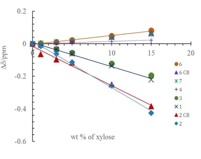
4.3.1.2 Proton Chemical Shift
The chemical shift ∆ of the resonances on the addition of carbohydrate was determined from the 1H spectra, this is the change for each resonance from the pure IL [C2mim] [OAc] “starting” position caused by the
addition of the carbohydrate. Figure 4.1 shows the labelling of proton resonances in the structure of IL [C2mim] [OAc]. The chemical shift of protons resonances was calculated using resonance peak 5 as the reference position, as described elsewhere 65. Protons of imidazolium ring [C2mim] have negative values of
∆ and a relatively large movement for peak 2, which is the most acidic proton. Peak 6 belongs to the anion [OAc] and peak 7 to a cation methyl group, and these both display positive values of ∆ . Figure 4.5 shows at
associated ions in the IL [C2mim] [OAc]. The reason for this is presumably the formation of hydrogen bonds between the IL and the OH groups from the carbohydrates and the disruption of the ion-ion interactions. It can be seen that cellobiose and xylose have almost identical effects, weight for weight, on the resonance frequencies of the ionic liquid protons.
[Figure 4.5 near here]
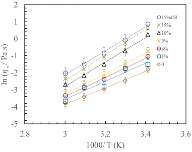
4.3.1.3 Viscosity
The viscosity measurements of different xylose concentrations (1%, 3%, 5%, 10% and 15%) were measured across the range of temperatures 20 °C to 60 °C inclusive. Figure 4.6 shows the experimental data for each concentration is plotted as (ln ) against inverse temperature. Viscosity values increase with xylose weight
fractions and decrease with temperature. It can be seen that the xylose solutions behave in a remarkably similar way to the cellobiose solutions.
[Figure 4.6 near here]
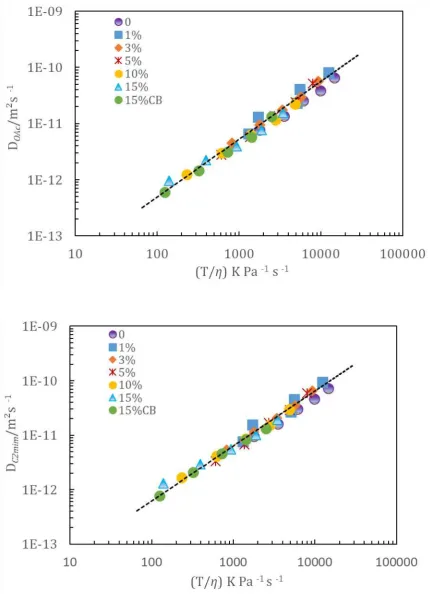
4.3.1.4 Stokes – Einstein Analysis
Stokes-Einstein relationship was employed to examine the relationship between the microscopic (diffusion)
and macroscopic (viscosity) properties of ions and molecules. The hydrodynamic radius, of ions was
calculated using Equation 4.3. The values of the effective hydrodynamic radius are for the anion 2.2 Å and
the cation 2.8 Å 6. These values of are used in Equation 4.2 with NMR diffusion data to determine the
correction term ƒ. Figure 4.7 (a, b) shows the correlation between translational diffusion of anions and cations and the ratio of temperature ( ) to the viscosity (Pa s) for the pure IL [C2mim] [OAc], 15% cellobiose and all the xylose concentrations. The cellobiose and xylose solutions follow the Stokes-Einstein Equation. All data, the pure ionic liquid, the 15% cellobiose and all the xylose solutions form a single master plot. From Figure 4.7 the gradients are used to determine the correction term, ƒ, as shown in Figure 4.8.
[Figure 4.7 near here]
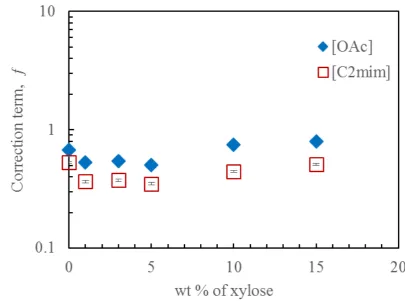
McLaughlin reported that when the sizes of ions are the same as that of the molecules of the solution, then
ƒ , but ƒ is equal to 1 when the diffusing particle is large compared to the molecules of the viscous
fraction of xylose. The ƒ for anions is and this indicates that the anions diffuse as expected. The cation f is lower, which indicates that the cations are diffusing faster than expected. This suggests that it is the faster diffusion of the cation that is the cause of the anomalous diffusion in this ionic liquid.
[Figure 4.8 near here]
4.3.1.5 NMR Low Field Relaxometry
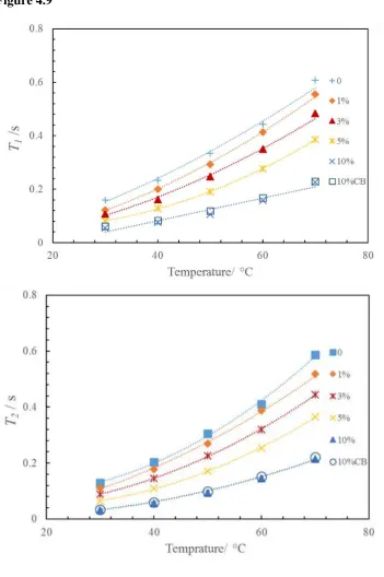
Low-Field (20MHz) NMR relaxation T1 and T2 of different xylose concentrations (1%, 3%, 5%, 10%, and 10% of cellobiose) were measured across the range of temperatures 30 °C to 70 °C. Low field NMR measurements have an inadequate chemical resolution to distinguish between ions; therefore, the calculated values of the relaxation times are an average across both ions. The values of T1 and T2 relaxation times increase with an increase in temperature, and decrease with increasing xylose concentration, indicating the loss of rotational mobility of the ions with increasing xylose. Figure 4.9 (a, b) shows T1 is very close to T2 for all the xylose samples, and that there is insignificant difference between 10% cellobiose results and the 10% xylose results. Across all our measurements cellobiose and xylose are practically indistinguishable. At low field relaxation, xylose is found to be in the liquid regime across all selected temperatures, meaning the rotation of the ions must be fast in comparison to the timescale set by the inverse of the Larmor frequency (20 MHz).
[Figure 4.9 near here]
4.3.1.6 Stokes-Debye-Einstein Analysis
As mentioned above, low field NMR has insufficient chemical resolution to distinguish between cations and
anion, therefore in the following analysis, the values of the hydrodynamic radii size, calculated are an
averaged value over both ions. Stokes- Einstein-Debye Equation 4.7 was applied to the NMR relaxation times
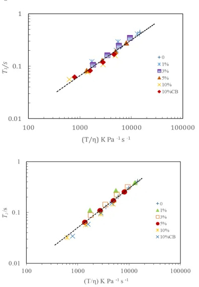
to calculate the value of the effective radius of the ions, . Figure 4.10a shows the dependence of relaxation
times T1 on the ratio of temperature to viscosity (T/ ) for 10% cellobiose and all the xylose concentrations.
All data collapse together to form one master curve, which shows how similar the cellobiose and xylose systems are. The gradient for each concentration is close to the expected unity from Equation 4.7. Figure 4.10b shows that same relationship holds almost as well for relaxation times T2. The slope for each concentration was used to calculate the value of the effective hydrodynamic radii using Equation 4.7.
Figure 4.11 shows the hydrodynamic radius calculated from the relaxation times T1 from the xylose solutions and the hydrodynamic radius determined from the sample density using12, which gives an average value of 2.5 Å. It can be seen from Figure 4.11that the value of the effective hydrodynamic radius increases somewhat with increase in concentration, though they are not far from the expected 2.5 Å, going between 3.5 Å to 4 Å. The size of ions does not in reality change, but their relative ease of motion within these solutions is changing and this is being quantified by this parameter.
[Figure 4.11 near here]
4.3.2 Xylan Results
4.3.2.1 NMR Diffusion
The influence of xylan on the diffusion properties of the ions of the IL [C2mim] [OAc] was examined using ¹H NMR spectroscopy, diffusion, and low field relaxometry, across the temperatures range (20 °C to 70 °C). Cellulose data, for comparison, has been taken from ref 49. Temperature increases both the diffusivity of cations [C2mim] and anions [OAc], but an increase in concentrations of xylan decreases them. The reason for this is that the viscosity is increased by the presence of xylan and decreased by increasing temperature and there is an inverse relationship between diffusion and viscosity, through the Stokes-Einstein relationship.
Figure 4.12 (a, b) shows the diffusion coefficients of cations and anions as a function of the inverse of temperature for all the xylan solutions. The values of diffusion coefficients of the imidazolium cations [C2mim] is close to that of the acetate anions [OAc].
[Figure 4.12 near here]
source, presumably a change in the local effective micro-viscosity. If the anion experienced more and/or stronger interactions with the carbohydrate, say via hydrogen – bonding, then this would preferentially reduce the diffusivity of the anion.
[Figure 4.13 near here]
4.3.2.2 Proton Chemical Shift
In Figure 4.14 the chemical shift results are displayed, for 40 , where is the resonance frequency for a
proton in parts per million (ppm), and ∆ indicates the change of this frequency from the pure IL [C2mim]
[OAc] positions, caused by the addition of xylan. The anion [OAc] forms hydrogen bonds with the carbohydrate, which moves it downfield, rather than remain associated with the protons in the imidazolium
ring [C2mim]. It is interesting to note that the ∆ on the addition of xylan is practically identical to the chemical shift movements on the addition of cellulose, implying that the dissolution process in both is similar.
[Figure 4.14 near here]
4.3.2.3 Viscosity
The measurements of viscosity of different xylan concentrations (1%, 3%, 5%, 10% and 15%) were measured across the range of temperatures from 20 °C to 60 °C inclusive. The viscosity dependence increases with adding xylan as would be expected. Figure 4.15 presents the experimental data for each concentration plotted
as zero-shear viscosity, against inverse temperature, K.
[Figure 4.15 near here]
4.3.2.4 Stokes-Einstein Analysis
Equation 4.312. Figure 4.16 (a, b) shows the correlation between the diffusion coefficients of anions and cations and the ratio of temperature to viscosity. The diffusion coefficients of cations and anion of IL [C2mim] [OAc] are slowly decreased with an increase in polymer concentration. However, this gradual reduction of diffusion coefficients came with a strong increase in viscosity.
[Figure 4.16 near here]
Figure 4.17 shows the correction term f for cation [C2mim] and anion [OAc] as a function of weight fraction of xylan. The correction term decreased with increased xylan concentration. It is interesting to note that the
anions have ƒ , so diffuse as expected, but the cations are less than one, this indicates the cations diffuse faster than expected. In Figure 4.16 the ƒ drops off with the increase in xylan concentration, this is due to the decoupling between the macroscopic and microscopic viscosities. Macroscopic entanglements are formed at concentrations above the overlap concentration and these dramatically increase the sample viscosities, but these large structures do not significantly alter the mobility of the ions, being quantified via the diffusion coefficients. This difference between what is happening microscopically and macroscopically is driving the decrease in f with increase in concentration.
[Figure 4.17 near here]
4.3.2.5 Low –Field Relaxometry
Figure 4.18 (a, b) show the low-field relaxation time T1 and T2 plotted as a function of temperature for 15% of cellulose and all the xylan concentrations. Here the relaxation T1 and T2 times are in the liquid regime, they increase in value with an increase in temperature. Figure 4.18 (a, b) displays the relaxation time measurements showing that T2 is slightly less than or approximately equal to T1 at 20 MHz. This suggests that rotational motion is the dominant mechanism for NMR relaxation 61. It can see that in Figure 4.18a that an increase in xylan concentration decreases T1. The relaxation time T1 is related to the mobility of the ions, with an increase here indicating an increase in mobility or, in other words, a decrease in the local micro-viscosity. The values of T1 for 15% of the cellulose are positioned between the 5% and 10% xylan concentration results. Therefore, the mobility of the ions at 15% of cellulose is higher compared to that of the ions in the 15% xylan solution.
4.3.2.6 Stokes-Debye–Einstein Analysis
Experimentally, relaxation times were measured across the temperature (70 °C - 30 °C). As before, Stokes- Einstein-Debye Equation was applied to calculate the values for the radius of ions in these solutions.
Figure 4.19 (a, b), presents the relationships between relaxation times and the ratio of temperature to viscosity. Figure 4.19a presents the relaxation time T1 for all xylan weight fraction combined from different temperatures giving a single master plot, while 15% of the cellulose is not connected with them. This is because cellulose
is the most effective at increasing the viscosity, due to its higher molecular weight as compared with the xylan.
Figure 4.19b shows that same relationship holds approximately as well for the relaxation time T2. The effective hydrodynamic radii for T1 and T2 is found using Equation 4.6. The values of hydrodynamic radii for all the xylan concentrations and all the temperatures T1 is roughly equal to or slightly higher than those found from the T2 analysis.
[Figure 4.19 near here]
Figure 4.20 shows the hydrodynamic radii, values of relaxation time T1 against xylan weight fractions
(1%, 3% and 5%), and is around 3Å, the values of hydrodynamic radii of ions in high concentrations 10% and
15% is around 2Å. The values of decreased with increasing xylan concentrations, because of the greater
increase of the macroscopic viscosity as compared to the microscopic viscosity that determines the rotational correlation times. In this analysis the hydrodynamic radius is quantifying this difference between what is occurring macroscopically and microscopically. 66
[Figure 4.20 near here]
4.4 Conclusion
NMR has been employed for the characterisation, through spectroscopy, diffusion and relaxation times, of a series of solutions of xylan and xylose in the ionic liquid [C2mim] [Oac]. In the xylose samples the self diffusion coefficients of the anions and cations were found to decrease with an increase in xylose weight
diffusion coefficient of anions to cations was less than 1 in all our samples. This is referred to as ‘‘anomalous’’ diffusion, because the anion is geometrically smaller than the cation and so would be expected to diffuse faster not slower than the cation. It has been suggested that this anion is diffusing as part of an aggregation67. Xylose data were compared to published cellobiose data49 to compare and contrast the influence of each on the ions. The changes in 1H chemical resonance frequencies ∆ for protons in the presence of xylose is almost identical to the chemical shift movements caused by cellobiose, which indicates that these carbohydrates have a very similar dissolving mechanism. The viscosity measurements and relaxation time data were used to measure the effective hydrodynamic radii, using the Stokes-Debye-Einstein relationship. The value of the hydrodynamic radii of the ions was between 3.5 Å to 4 Å in the xylose solutions, which is quite close to the expected 2.5 Å.
Solutions of xylan in the ionic liquid [C2mim] [OAc] were examined and these results were compared with published data on solutions of cellulose in the same ionic liquid. The mobility of ions in xylan solutions decreased with increasing concentration, due to the viscosity being increased by the presence of xylan. The ratio of the diffusion coefficient of anion to cation in the xylan mixtures is, as with the xylose and cellulose mixtures, less than 1. The proton chemical shift analysis indicates that in the cellulose and xylan mixtures the dissolution mechanism is similar; in the case of xylan the cation and anion are though more equally affected by the addition of this carbohydrate than they were by the addition of cellulose, which affects the anion
resonance frequency preferentially more than the cation weight for weight.
The viscosity data was used with diffusion to measure the correction term f in the Stokes-Einstein equation 4.2, and was used with the NMR relaxation times to calculate the effective hydrodynamic radii for the ions. In the xylan system, it was found that the correction term ƒ reduced dramatically with the addition of xylan; this is because of the decoupling between the macroscopic and microscopic viscosities, and in particular the role of entanglements in dramatically increasing the zero shear rate viscosity. The values of hydrodynamic radii of ions were calculated using Equation 4.7. The values found were between 3Å and 2Å in the xylan mixtures.
Acknowledgement
M.E.R. is a Royal Society Industry Fellow (IF120090). The data for this article can be found at http://doi.org/10.5518/???.
W.M.E is funded by Minister of High Education and Libyan Embassy London-Cultural Affairs.
References*
*For books in the Issues in Toxicology series, please include the full article title and page range.
For books in the Food and Nutritional Components in Focus (Editor: Victor Preedy), please use Harvard referencing and include the full article title and page range.
1. L. Hall, in Advances in carbohydrate chemistry, Elsevier, 1964, vol. 19, pp. 51-93. 2. P. J. Hore, Nuclear magnetic resonance, Oxford University Press, USA, 2015. 3. H. Y. Carr and E. M. Purcell, Physical review, 1954, 94, 630-638.
4. R. M. Mazo, Brownian motion: fluctuations, dynamics, and applications, Oxford University Press on Demand, 2002.
5. D. Le Bihan and P. J. Basser, Diffusion and perfusion magnetic resonance imaging, 1995, 5-17. 6. C. A. Hall, K. A. Le, C. Rudaz, A. Radhi, C. S. Lovell, R. A. Damion, T. Budtova and M. E. Ries,
J.Phy. Chem. B, 2012, 116, 12810-12818.
7. A. Macchioni, G. Ciancaleoni, C. Zuccaccia and D. Zuccaccia, Chemical Society Reviews, 2008, 37, 479-489.
8. W. S. Price, Diff. fund, 2005, 2, 1-19.
9. R. T. Boeré and R. G. Kidd, in Annual reports on NMR spectroscopy, Elsevier, 1983, vol. 13, pp. 319-385.
10. P. T. Callaghan, Principles of nuclear magnetic resonance microscopy, Oxford University Press on Demand, 1993.
11. R. Kimmich, NMR: tomography, diffusometry, relaxometry, Spr. Sci & Bus. Med, 2012. 12. E. McLaughlin, Transactions of the Faraday Society, 1959, 55, 28-38.
13. J. C. Li and P. Chang, The Journal of Chemical Physics, 1955, 23, 518-520.
14. B. Blicharska, H. Peemoeller and M. Witek, Journal of Magnetic Resonance, 2010, 207, 287-293. 15. N. Bloembergen, E. M. Purcell and R. V. Pound, Physical review, 1948, 73, 679.
16. P. Wasserscheid and W. Keim, Angewandte Chemie International Edition, 2000, 39, 3772-3789. 17. P. Walden, Bull. Acad. Imper. Sci.(St. Petersburg), 1914, 1800.
18. H. Tokuda, K. Hayamizu, K. Ishii, M. A. B. H. Susan and M. Watanabe, The Journal of Physical Chemistry B, 2004, 108, 16593-16600.
19. J. G. Huddleston, A. E. Visser, W. M. Reichert, H. D. Willauer, G. A. Broker and R. D. Rogers, Green chemistry, 2001, 3, 156-164.
20. B. D. Rabideau, A. Agarwal and A. E. Ismail, The Journal of Physical Chemistry B, 2014, 118, 1621-1629.
22. T. Heinze, S. Dorn, M. Schöbitz, T. Liebert, S. Köhler and F. Meister, 2008.
23. C. Olsson, A. Hedlund, A. Idström and G. Westman, Journal of Materials Science, 2014, 49, 3423-3433.
24. C. Graenacher, US Patent, No. 1943176, 1934.
25. R. P. Swatloski, S. K. Spear, J. D. Holbrey and R. D. Rogers, Journal of the American chemical society, 2002, 124, 4974-4975.
26. R. D. Rogers and K. R. Seddon, Science, 2003, 302, 792-793.
27. I. Kilpeläinen, H. Xie, A. King, M. Granstrom, S. Heikkinen and D. S. Argyropoulos, Journal of agricultural and food chemistry, 2007, 55, 9142-9148.
28. S. Bylin, C. Olsson, G. Westman and H. Theliander, BioResources, 2014, 9.
29. N. Sun, M. Rahman, Y. Qin, M. L. Maxim, H. Rodríguez and R. D. Rogers, Green Chemistry, 2009, 11, 646-655.
30. M. B. Shiflett and A. Yokozeki, Journal of Chemical & Engineering Data, 2008, 54, 108-114. 31. J. Vitz, T. Erdmenger, C. Haensch and U. S. Schubert, Green chemistry, 2009, 11, 417-424. 32. H. Wang, G. Gurau and R. D. Rogers, Chemical Society Reviews, 2012, 41, 1519-1537.
33. D. Bowron, C. D’Agostino, L. Gladden, C. Hardacre, J. Holbrey, M. Lagunas, J. McGregor, M. Mantle, C. Mullan and T. Youngs, The Journal of Physical Chemistry B, 2010, 114, 7760-7768. 34. H. V. Scheller and P. Ulvskov, Annual review of plant biology, 2010, 61.
35. B. Gyurcsik and L. Nagy, Coordination chemistry reviews, 2000, 203, 81-149. 36. I. Siró and D. Plackett, Cellulose, 2010, 17, 459-494.
37. A. C. O'sullivan, Cellulose, 1997, 4, 173-207. 38. A. Payen, Comptes rendus, 1838, 7, 1052-1056.
39. D. Klemm, B. Heublein, H. P. Fink and A. Bohn, Angewandte Chemie International Edition, 2005, 44, 3358-3393.
40. R. H. Atalla and D. L. Vanderhart, Science, 1984, 223, 283-285.
41. A. S. Gross and J.-W. Chu, The Journal of Physical Chemistry B, 2010, 114, 13333-13341. 42. M. Luo, A. N. Neogi and H. West, Journal, 2010.
43. V. Finkenstadt and R. Millane, Macromolecules, 1998, 31, 7776-7783.
44. L. Day and I. McNeil, Biographical dictionary of the history of technology, Routledge, 2002. 45. J. Sundberg, G. Toriz and P. Gatenholm, Cellulose, 2015, 22, 1943-1953.
46. A. E. da Silva, H. R. Marcelino, M. C. S. Gomes, E. E. Oliveira, T. Nagashima Jr and E. S. T. Egito, in Products and Applications of Biopolymers, InTech, 2012.
47. K. Petzold-Welcke, K. Schwikal, S. Daus and T. Heinze, Carbohydrate polymers, 2014, 100, 80-88. 48. S. Daus and T. Heinze, Macromolecular Bioscience, 2010, 10, 211-220.
49. M. E. Ries, A. Radhi, A. S. Keating, O. Parker and T. Budtova, Biomacromolecules, 2014, 15, 609-617.
50. S.-J. Ha, J. M. Galazka, S. R. Kim, J.-H. Choi, X. Yang, J.-H. Seo, N. L. Glass, J. H. Cate and Y.-S. Jin, Proceedings of the National Academy of Sciences, 2011, 108, 504-509.
51. J. E. Tanner, The Journal of Chemical Physics, 1970, 52, 2523-2526.
52. K.-D. Merboldt, W. Hanicke and J. Frahm, Journal of Magnetic Resonance (1969), 1985, 64, 479-486.
53. R. Cotts, M. Hoch, T. Sun and J. Markert, Journal of Magnetic Resonance (1969), 1989, 83, 252-266. 54. E. O. Stejskal and J. E. Tanner, The journal of chemical physics, 1965, 42, 288-292.
55. A. Haase and J. Frahm, Journal of Magnetic Resonance (1969), 1985, 64, 94-102.
56. J. Frahm, K. Merboldt, W. Hänicke and A. Haase, Journal of Magnetic Resonance (1969), 1985, 64, 81-93.
57. S. M. Green, M. E. Ries, J. Moffat and T. Budtova, Scientific Reports, 2017, 7, 8968. 58. W. S. Price, Concepts in Magnetic Resonance Part A, 1997, 9, 299-336.
61. P. J. Hore, Jones, J. A., Wimperis, S.,, 3-6. 62. D. Freude, Spectroscopy, 2006, 1-29.
63. J. Xie and Y.-C. Jin, Engineering Applications of Computational Fluid Mechanics, 2016, 10, 111-129. 64. G. Annat, D. R. MacFarlane and M. Forsyth, The Journal of Physical Chemistry B, 2007, 111,
9018-9024.
65. C. S. Lovell, A. Walker, R. A. Damion, A. Radhi, S. F. Tanner, T. Budtova and M. E. Ries, Biomacromolecules, 2010, 11, 2927-2935.
66. W. Burchard and M. Eisele, Pure and applied chemistry, 1984, 56, 1379-1390.
Figure Captions
Figure 4.1 The chemical structure of 1-ethyl-3-methylimidazolium acetate, cations [C2mim]+ and anion
[OAc]– with the labelling of NMR resonance peaks (1-7).
Figure 4.2 The chemical structure of carbohydrates (a) cellulose (b) xylan (c) D-xylose and (d) cellobiose.
Figure 4.3 Arrhenius plots for the diffusion coefficients of (a) anions [OAc] and (b) cations [C2mim], for
15% cellobiose and all xylose weight fraction. Solid lines represent linear fits to the data and error bars are within the symbols used. [CB] means cellobiose.
Figure 4.4 The ratio of diffusion coefficients of anion to cation as a function of temperature for xylose and
cellobiose. Solid lines correspond to linear fits and error bars are within the symbols sizes. [CB] means cellobiose.
Figure 4.5 The chemical shift of protons resonances ∆ (ppm) versus weight fraction of xylose and cellobiose
[CB] at 40 °C. Error bars are within the symbols sizes.
Figure 4.6 The logarithmic plots of the viscosity of pure [C2mim] [OAc] and 15% cellobiose and xylose in
IL [C2mim] [OAc] solutions versus inverse temperature. Lines are linear approximations. Error bars are within the size of the symbols used. [CB] means cellobiose.
Figure 4.7 NMR diffusion coefficients of (a) cations and (b) anions against the ratio of temperature to the
viscosity of pure IL [C2mim] [OAc] and 15% cellobiose and all xylose concentrations. Dashed lines are provided as visual guide and error bars are within the symbols sizes. [CB] means cellobiose.Figure 4.8 The
correction term, ƒ, of cations and anions as a function of weight fraction of xylose. The error bars are in the
same size of symbols used
Figure 4.9 NMR relaxation times T1 and T2 as a function of temperature at 20 MHz, for all xylose
concentrations with 10% cellobiose. Error bars are within data size and the dashed lines to guide the eye. [CB]
means cellobiose.
Figure 4.10 The relaxation times T1 and T2 dependence on the ratio of temperature to viscosity for 10%
Figure 4.11 The experimental values (blue diamond) of effective hydrodynamic of radii as a function of the
weight fractions of xylose solutions calculated by Equation 4.2. The solid red line shows the hydrodynamic radius of the averaged ions of pure IL [C2mim] [OAc] measured by using Equation 4.3. The errors are within the size of data points. The solid blue line is a linear fit to the data points.Figure 4.12 The diffusion coefficients of cations [C2mim] (a) and anion [OAc] (b) as a function of the inverse of temperature for 15% cellulose and xylan concentrations. Dashed lines are linear fits to the data. C means cellulose data.Figure 4.13 Ratio of the diffusion coefficient of the anion to the cation as a function of temperature. Solid lines correspond to linear fits. Error bars are within the symbols sizes.Figure 4.14 The chemical shift of protons resonances ∆ (ppm) versus weight fraction of xylan [X] and cellulose [C] at 40 °C. Error bars are within the symbols sizes. The lines are guides to eye.
Figure 4.15 Logarithmic plots of the viscosity of pure [C2mim] [OAc] and 15% cellulose and xylan in IL
[C2mim] [OAc] solutions versus inverse temperature. Lines are linear approximations. Error bars are within the symbol sizes. [C] means cellulose data.Figure 4.16 NMR diffusion coefficient of anions (a) and cations (b) against the ratio of temperature to the viscosity of pure IL [C2mim] [OAc] and 15% cellulose and all xylan concentrations. Solid lines are provided as a visual guide and error bars are within the symbols sizes. [C] means cellulose data.Figure 4.17 The correction term ƒ as a function of weight fraction of xylan. The solid lines are provided as a visual guide. Error bars are within the symbols sizes.Figure 4.18 Arrhenius plots for relaxation times T1 (a) and T2 (b) against the inverse of temperature, for 15% cellulose and all xylan weight fractions. Dashed lines represent straight line fits to the data, and error bars within the symbols sizes. [C]
23
24
Figure 4.2
Cellulose
Xylan
Xylose
[image:25.595.32.290.115.700.2]25
26
27
28
29
30
[image:31.595.37.443.140.441.2]31
[image:32.595.40.392.94.623.2]32
33
34
Xylan
35
36
[image:37.595.38.414.88.381.2]37
38
39
40
41
42