Investigating Bayesian optimization for rail network optimization

optimization

.

White Rose Research Online URL for this paper:

http://eprints.whiterose.ac.uk/151331/

Version: Published Version

Article:

Hickish, R. orcid.org/0000-0003-2526-7863, Fletcher, D.I. and Harrison, R.F. (2019)

Investigating Bayesian optimization for rail network optimization. International Journal of

Rail Transportation. ISSN 2324-8378

https://doi.org/10.1080/23248378.2019.1669500

[email protected] https://eprints.whiterose.ac.uk/ Reuse

This article is distributed under the terms of the Creative Commons Attribution (CC BY) licence. This licence allows you to distribute, remix, tweak, and build upon the work, even commercially, as long as you credit the authors for the original work. More information and the full terms of the licence here:

https://creativecommons.org/licenses/

Takedown

If you consider content in White Rose Research Online to be in breach of UK law, please notify us by

Full Terms & Conditions of access and use can be found at

https://www.tandfonline.com/action/journalInformation?journalCode=tjrt20

International Journal of Rail Transportation

ISSN: 2324-8378 (Print) 2324-8386 (Online) Journal homepage: https://www.tandfonline.com/loi/tjrt20

Investigating Bayesian Optimization for rail

network optimization

Bob Hickish, David I. Fletcher & Robert F. Harrison

To cite this article: Bob Hickish, David I. Fletcher & Robert F. Harrison (2019): Investigating Bayesian Optimization for rail network optimization, International Journal of Rail Transportation, DOI: 10.1080/23248378.2019.1669500

To link to this article: https://doi.org/10.1080/23248378.2019.1669500

© 2019 The Author(s). Published by Informa UK Limited, trading as Taylor & Francis Group.

Published online: 14 Oct 2019.

Submit your article to this journal

Article views: 45

View related articles

Investigating Bayesian Optimization for rail network

optimization

Bob Hickish a_{, David I. Fletcher} a_{and Robert F. Harrison} b

a_{Department of Mechanical Engineering, The University of She}

ffield, Sheffield, UK;b_{Department of} Automatic Control and Systems Engineering, The University of Sheffield, Sheffield, UK

ABSTRACT

Optimizing the operation of rail networks using simulations is an on-going task where heuristic methods such as Genetic Algorithms have been applied. However, these simulations are often expensive to compute and consequently, because the optimization methods require many (typically >104) repeat simulations, the computational cost of optimization is dominated by them. This paper examines Bayesian Optimization and benchmarks it against the Genetic Algorithm method. By applying both methods to test-tasks seeking to maximize passenger satisfaction by optimum resource allocation, it is experimentally determined that a Bayesian Optimization imple-mentation finds ‘good’solutions in an order of magnitude fewer simulations than a Genetic Algorithm. Similar improvement for real-world problems will allow the predictive power of detailed simulation models to be used for a wider range of network optimization tasks. To the best of the authors’knowledge, this paper documents thefirst application of Bayesian Optimization within thefield of rail network optimization.

ARTICLE HISTORY

Received 3 April 2019 Revised 6 September 2019 Accepted 15 September 2019

KEYWORDS

Bayesian Optimization; Genetic Algorithm; rail; network; optimization; simulation

1. Introduction

Improving the operation of rail networks is an on-going challenge for rail service providers such as train operating companies and infrastructure managers. In Great Britain, there is evidence that service providers have recognized the importance of improving the performance of their network from the passenger perspective. For example, customer experience is identified as one of four strategic goals by the Technical Leadership Group [1]. To assist with improving network operation, detailed models, for example by Yao et al. [2] and Landex and Nielsen [3], have been developed to predict network performance from the passenger perspective. The optimization of detailed rail network models will enable service providers to improve the performance of their network from the passenger perspective. However, the two well-established methods within thefield of rail network optimization [Mathematical Programming and Genetic Algorithms (GAs)] are poorly suited for this task. Mathematical Programming requires specific model formulations that make it difficult to adequately capture the detail of individual passenger journeys [4]. GAs can be applied with any model

CONTACTDavid I. Fletcher d.i.fletcher@sheffield.ac.uk Department of Mechanical Engineering, The University of Sheffield, Mappin Street, Sheffield S1 3JD, UK

https://doi.org/10.1080/23248378.2019.1669500

© 2019 The Author(s). Published by Informa UK Limited, trading as Taylor & Francis Group.

formulation (e.g. an agent-based simulation of individual passenger journeys) to find solutions that are approaching optimal, although without any formal certainty that an optimum is found, that is ‘good’ solutions are identified. However, because a GA requires many computations of a model (e.g. an agent-based simulation) there is a need to maintain a low computational cost for each model evaluation. This require-ment is in conflict with the use of detailed simulation models because, in the case where many passengers are being simulated, it is difficult to adequately capture passenger journeys at low computational expense.

Bayesian Optimization (BO) has the potential to find similarly good solutions to a GA, but in fewer model computations because it uses a predictive model of the search space to target the selection of new candidate solutions for evaluation. GAs are well suited to tasks with cheap-to-compute models and large numbers of optimization variables, while BO has the potential to be computationally cheaper for tasks with an expensive-to-compute model and few optimization variables (many established imple-mentations currently perform well for less than approximately 25). This reduction in computational requirement could enable the wider use of more detailed models when optimizing a rail network, or allow good solutions to be found at lower computational cost than with a GA. BO might therefore be an additional optimization tool for rail network operators, especially considering that implementations are being developed to increase the upper limit on the number of optimization variables and reduce the computational cost of calculating its inherent predictive model. This paper investigates BO and experimentally compares it against a GA on a range of test-tasks involving a passenger rail network where there is a large number of operational options, that is potential or candidate solutions to the network operation problem. Following a brief review of GA and BO methods, this paper compares the computational costs of both methods. To the best of the authors’ knowledge, this paper documents the first application of BO within the field of rail network optimization.

1.1. Genetic Algorithm for optimizing rail networks

1.2. Applications of Bayesian Optimization

There are many examples of BO being used to select the hyperparameter values of expensive-to-compute machine learning algorithms [10,11]. Applications outside the

field of machine learning are less common but can be categorized into two purposes:

● To maximize the agreement between a model and observed data by optimally

fitting model parameters.

● To maximize the performance of a real-world entity by optimizing design and operational model parameters.

In this paper, the BO and GA methods are compared for the latter purpose. An example of this type of application is the use of BO by Candelieri et al. [12] to maximize the performance of a simulated water distribution network by optimizing the pump schedule. Candelieri et al. use BO because of its advantages when applied with expensive-to-compute simulations. For an alternative case, Lisicki et al. [13] report that BOfinds a solution which performs approximately 50% better than that found by random search with an equal number of evaluations. Neither Candelieri et al. or Lisicki et al. make a quantitative comparison of BO against a sophisticated optimization method such as GA and at the time of writing, the only identified application of BO in a transportation network setting is by Schultz and Sokolov [14] who optimize the parameters of trans-portation network simulators to maximize agreement with observed data.

An explicit comparison between GAs and BO is presented by Trotter et al. [15] to compare both approaches for maximizing the performance of a distributed computing system. However, it can be inferred that this comparison is not made for an equal budget of candidate solution evaluations and is therefore difficult to generalize from. Chandrashekaran et al. [16] report the number of candidate evaluations in a comparative optimization of a speech recognition model. However, the use of a very small population size again limits the generalizability of the conclusions.

2. Genetic Algorithm and Bayesian Optimization

As a basis for equitable comparison of BO and GA we consider the general task of selecting the optimum value of a vector,x, which maximizes a non-negative objective

function, fð Þx . In the case of a rail network, the objective function quantifies the

performance of the network. The vector, x

; comprises n elements and exists in the n-dimensionalsearch space, X, bounded by the upper and lower bounds (constraints) of each optimization variable, xi;i¼1;2;. . .n, leading to the optimization task given by (1) subject to constraints (2) and (3).

x¼arg max

x2X

fð Þx (1)

gjð Þ ¼x 0for j¼1;2; . . .

; p (2)

hkð Þ x 0for k¼1;2; . . .

Where:x is the global optimum and there arepequality constraints on x, defined by

gjð Þx , andqinequality constraints, defined byh_kð Þx . For a case requiring minimization

offð Þx , maximization of fð Þx would be used.

A brief description of both GAs and BO is given in the following subsections. More comprehensive descriptions of GAs can be found in Goldberg [17] and Mitchell [18], and of BO in Shahriari et al. [19]. Note that within the GA literature, the objective function is usually referred to as a‘fitness function’, however‘objective function’is used here for both cases for consistency.

2.1. Genetic Algorithm

A GA is a simple computational model of the process of natural selection in an evolving population. At every iteration, a GA evaluates the objective function for every candidate solution within a population. By selecting the candidates with the best objective function scores and‘mating’them, the population at later generations exhibits more characteristics of candidates with good objective function scores and converges towards the optimum. ‘Mutation’is used to allow a GA to‘explore’the search space. The GA method can be applied to many types of optimization task with any number of optimization variables and, because it requires many (typically >104) evaluations offð Þx , it is well suited to tasks where

fð Þx is cheap-to-compute. Algorithm 1 presents pseudo-code for a simple GA. An

important control parameter of the algorithm is the population size, P. The algorithm iterates depending on a conditional statement at line 4 that is often related to the objective function scores of the candidates found so far, or, the computational resources used. The number of algorithm iterations used by a GA,IGA, is thefinal value ofiin Algorithm 1. At every iteration all of the candidates in a generation are evaluated so the number of objective function evaluations,ηGA_{, required, is given by:}

ηGA ¼ IGAP (4)

Algorithm 1: Genetic Algorithm (P)

1. Initialize population,G1, with Pcandidates

2. Evaluate objective function for every candidate in G1 3. i¼1

4. while _{Is-Not-Terminatedði} ;GiÞ

5. Giþ1¼Evolveð ÞGi //select, mate and mutate candidates

6. Evaluate objective function for every candidate inGiþ1 7. i¼iþ1

8. end

9. Return best candidate evaluated so far

2.2. Bayesian Optimization

to compute and is continuous so it is‘easier’tofind its maximum. To create the proxy function, a probabilistic model is inferred from previous evaluations of the objective function’s value at different locations in the search space. For this model, it is common [10] to use a Gaussian Process (GP) regression model as is the case considered here. The proxy function, μð Þx , and its uncertainty, σð Þx , are respectively the mean and

standard deviation of the GP model. At each iteration of a BO algorithm, the objective function is evaluated and the new data is used to update the probabilistic model and, hence, the proxy function. Information from the proxy function is used to create an

acquisition function, whose global maximum indicates where in the search space the

objective function should next be evaluated. The acquisition function is important to the success of BO because it‘guides’the search, but finding its maximum increases the computational expense of the whole process, particularly for tasks with more than approximately 25 dimensions [20]. Nonetheless for tasks with less than approximately 25 dimensions, it is often cheaper than evaluating an expensive-to-compute objective function and consequently the BO method is often well suited to task of this type. For higher dimension tasks, BO implementations are still being developed that keep the cost of maximizing the acquisition function reasonable, for example Li et al. [21]. Algorithm 2 presents pseudo-code outlining BO and is further described in the appendix. BO only uses one objective function evaluation per iteration; therefore, the number of expensive-to-compute evaluations,ηBO_{, is equal to the value ofi at the end of Algorithm 2.}

Algorithm 2: Bayesian Optimization()

1. Initialize candidate,x₁

2. y1¼fð Þx₁ //sample objective function

3. D¼ x₁

;y1

½ Š//data set of corresponding x and y values 4. Calculateμð Þx andσð Þx usingD

5. i¼1

6. while_{Is-Not-Terminatedði;DÞ} 7. Create acquisition function,αð Þx

; usingμð Þx andσð Þx 8. x_iþ1¼arg max

x2X αð Þx

9. yiþ1 ¼fðx_iþ1Þ

10. D¼fD;½xiþ1;yiþ1Šg//augment new data to data set 11. Calculateμð Þx andσð Þx using D

12. i¼iþ1 13. end

14. Return best candidate evaluated so far

2.3. Comparing the computational cost of Genetic Algorithms and Bayesian Optimization

the cost of a single evaluation, γ. Note that when variables apply to both approaches, superscripts are used to denote variables specific to an approach. Because of the multiplier, P, in (4), it is expected that ηGA>ηBO and consequently that ΓGA > ΓBO. However, because BO involves the expensive step of maximizing an acquisition func-tion at every iterafunc-tion, GA_<BO _{resulting in a trade-off between the low algorithm}

cost, high objective function evaluation cost of GAs and the high algorithm cost, low objective function evaluation cost of BO. The case of BO being cheaper than a GA is captured by (5) which demonstrates that the value ofγis important for determining the best method. Note that γ is constant between the approaches and is assumed to be constant for allx.

BOþγηBO< GAþ γηGA (5)

Because the number of objective function evaluations and the number of algorithm iterations are related, the value of is dependent on η. In the case of a GA this is a linear dependency. However in the case of BO with a GP model, calculating the model withi data points requires inversion of a square matrix of dimensioni. The computa-tional cost of this isO i_{ð Þ}3 _{. Consequently, the value of}BO_{may become fourth order for}

largeηBO_{. However, developing methods to compute large matrix inversions at reduced}

cost is an active area of research [22,23] so this is not seen as a fundamental limitation of BO. Furthermore, although not utilized here with BO, Gardner et al. [24] present a method using parallel computing techniques that can reduce the cost of computing a GP model can be reduced toO i_{ð Þ}2

:

3. Experimental comparison of a Genetic Algorithm and Bayesian Optimization

For an experimental comparison, specific GA and BO implementations were applied to a range of test-tasks involving an expensive-to-compute objective function that simu-lates passengers using a rail network and captures their satisfaction. For an unambig-uous comparison, the globally optimal solutions (x*) must be known. For this reason,

the test-tasks have been chosen so thatx* can be calculated analytically.

3.1. The test-tasks

Two examples of demands in rail network operation are:

● The allocation offinite rolling stock between scheduled train paths [25].

● The choice of which areas of the rail network should receive investment for increased line speed [26].

of the test-tasks, any number of carriages greater than zero can be allocated to a train provided that the limit on the total number of carriages available is not exceeded. The passenger capacity of a train affects the performance of the network because it is related to the comfort and duration of passenger journeys. A track section linking adjoining stations in the test-task network is defined as alinethat is homogenous and bi-directional. In these test-tasks, the line speed can be one of two alternatives: a ‘basic’ level and an ‘upgraded’ level. The line speed affects passenger journey times and hence the network performance. For the test-tasks, the carriage allocations and line speeds are the optimization variables whose values are chosen to maximize network performance from the perspective of passengers and for the greatest number of passengers.

The family of networks used in the test-tasks are chosen to have a high degree of symmetry so that the global optimum can be calculated analytically. A radial network design is used where the central station is connected to outer stations by two lines. The networks are named B2, B3, and B4 where the number refers to the number of links in the network.

Figure 1shows the topographies of the networks with a circle representing a station and a connecting edge representing a railway line. Each line within the network has one train operating upon it and the trains do not transfer between lines.Table 1displays the number of lines and trains in the test-networks and how this controls the number of optimization variables. The number of trains within the network is equal to the number of lines within the network so we only state the number of trains from here on in. The

Figure 1.Topographical representation of three different sized networks from the family of networks used for test-tasks. A circle represents a station. An edge between two stations represents a bi-directional line upon which trains travel. The name of the network topography is displayed below each network.

Table 1. The number of lines and trains for the three different sized networks used in test-tasks.

trains operate to a symmetrical timetable and all lines have a dedicated platform at their connected station. The passengers using the network (defined as the passenger load) have a symmetrical origin-destination-time matrix. It is recognized that these networks are simplistic and idealized relative to real world networks, however their properties are sufficient to test the relative performance of the GA and BO methods in preparation for application to more realistic cases.

Although the BO implementation tested here cannot be scaled to tasks representing the whole GB network in this way, that is every individual line represented by an optimization variable, there are opportunities at regional and individual train opera-tor scales. While these tasks present a computational challenge at present, new developments such as a BO implementation allowing more optimization variables might be used [21].

3.2. Formal definition of the test-tasks

Here the general definition of constrained optimization given by (1), (2) and (3) is modified to the family of test-tasks described in the previous section. The tasks can be described as optimizing the distribution ofMidentical carriages amongstRtrains and selecting the line speed of each of theLlines fromSdiscrete choices. The vector,x, isR + Ldimensional with

x1;x2;. . .:xR describing the number of carriages allocated to trains 1 to R and xRþ1;xRþ2. . .xRþL describing the line speeds of lines 1 toL. The form ofxis therefore shown by:

x¼ x₁

;x2;. . .:xR; xRþ1;xRþ2. . .xRþL

½ Š (6)

The general objective function,fð Þx , is modified to the specific functionFðx;λ;θÞwhich

quantifies network performance from the passenger perspective where λdescribes the network parameters other than carriage allocations and line speeds (e.g. station loca-tions, train performance, timetable) andθdescribes the passenger load. Neitherλorθ are optimized. The test-tasks have no constraints placed on the choice of line speed (i.e. all lines can have the maximum line speed). Furthermore, because there is no penalty associated with increasing the line speed, the globally optimal solution will have all line speeds maximized – in real-world application costs such as energy and wear and tear are associated with higher line speeds so a cost function penalizing these aspects could be accommodated. However, in this task, there is a constraint on the carriage alloca-tions that a maximum of M carriages can be distributed between all the trains, captured by:

Xk¼R

k¼1

xkM (7)

A negative number of carriages cannot be allocated, this is captured by (8), and the limit on the number of choices of line speed is captured by (9).

0xk for 1kR (8)

The formal definition of the family of test-tasks can therefore be written as (10) subject to (7)–(9).

x¼arg max

x2X

Fðx;λ;θÞ (10)

3.3. Quantifying solution performance

The objective functionFðx;λ;θÞquantifies the performance of a network, described by xandλand carrying passenger load,θ, from the passenger perspective. To calculate the

value of the objective function, an agent-based simulation is used that models indivi-dual passengers using a rail network to make their journeys. The quality of the individual passenger journey is quantified and all passenger journeys aggregated to give a network score. This model has been developed by the authors and is fully described by Hickish et al. [27]. The value ofFðx;λ;θÞis expressed on the percentage

scale from 0 to 100%. 100% relates to the known global maximum, 0% relates to the known global minimum. The experimental parameter,F, is introduced to describe the target performance of the solution. F is the smallest value of Fðx;λ;θÞ that must be

found by an implementation before terminating with a result. Candidates (x) for which

Fðx;λ;θÞ Fare referred to asacceptable solutions.

3.4. Methodology

Experiments were carried out in MATLAB 2017b using its proprietary optimization functions, here denotedgaandbayesopt. The number of objective function evaluations used bygaandbayesoptwas measured for eight‘jobs’, that is a specific combination of test-task and F _{that is input to a function. A test-task is defined by the number of} trains in the network and the number of carriages to be allocated. To collect experi-mental data, a job is submitted to a function and the algorithm iterates until an acceptable solution is found or a limit on the number of objective function evaluations is reached. The number of objective function evaluations required by the algorithm is recorded for the experiment. Because the algorithms are non-deterministic it is neces-sary to repeat, independently, each experiment multiple times and describe distribu-tions. For comparison between the GA and BO methods, identical tasks are submitted to the algorithms. Because the control parameters of each implementation differ, attainment of identical terminal objective function values is used to ensure like-for-like comparison.

3.5. Results

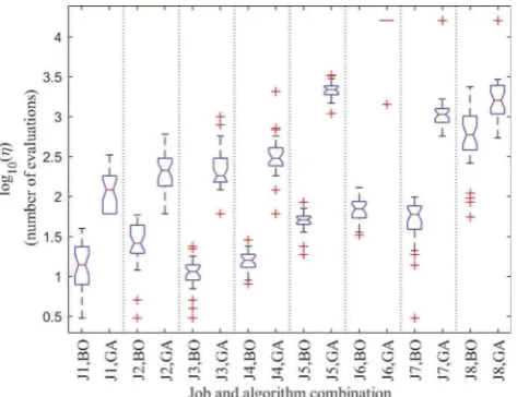
Figure 2is a box and whisker plot comparing the number of evaluations required byga

and bayesopt, ηGA _{and η}BO_{, for eight jobs. Each box and whisker represents, on}

a logarithmic scale, a distribution from 32 repeats of an experiment. Distributions for the same job are plotted next to each other and separated by vertical dashed lines to allow easy comparison. The job and method that each distribution relates to is dis-played on the x-axis. The notation ‘J1’, ‘J2’, ‘J3’, etc. can be cross-referenced against Table 2to observe the experimental parameters defining the job. A full factorial design for three experimental parameters and two levels has been used. An arbitrary limit of 1.6 × 104objective function evaluations was used which corresponds to approximately 48 hours of objective function computation time per experiment. This limit only affects the median and quartile results of‘J6,GA’, but still allows a discernible difference with ‘J6,BO’. The box notches indicate a 95% confidence interval of the median. When comparing distributions for the same job but different methods, there are no cases in which the notches overlap indicating that, on average, ηGA

>ηBO with approximately 95% confidence [28]. The features of the‘J6,GA’plot are indiscernible because for 31 of

Figure 2. Box plots showing the distribution of the number of objective function evaluations required, η, for eight different jobs. The y-axis is on a log10 scale. Each box plot represents a distribution of 32 repeat experiments.Table 2displays the experimental parameters of each job described by the‘J number’. The whiskers extend to a maximum of the inter-quartile range below and above the 25th and 75th percentiles respectively. Data outside this range is considered an outlier and is shown by a cross.

Table 2. The experimental parameters of the eight jobs for which the BO and GA methods are compared inFigure 2.

J1 J2 J3 J4 J5 J6 J7 J8

Trains 4 4 4 4 8 8 8 8

Carriages 8 8 48 48 8 8 48 48

the experiments, the GA implementation did notfind an acceptable solution within the limit of objective function evaluations. Comparing all eight jobs, the mean of the factor differences between ηBO _{and η}GA _{is 43 with a standard deviation of 76. Furthermore,}

excluding J6 where the comparison is not valid, the inter-quartile ranges of the BO distributions are narrower (the log scale of the y-axis means this is true even for J7), indicating that BO is more consistent in the number of objective function evaluations required tofind an acceptable solution.

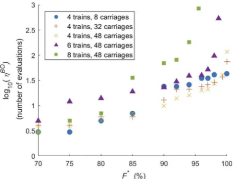
3.5.1. The number of objective function evaluations and target performance Following the comparison to a GA, the relationship between the number of objective function evaluations required by bayesopt and the target solution performance was investigated. Five different tasks were considered and they-axis value ofFigure 3is the logarithm of the median from 24 repeats of the experiment.

The data shows a positive relationship between F and log₁₀ðηBO_{Þ that is at least}

linear. This means that the relationship betweenFandηBO_{is at least exponential. The}

increase inηBOis more sensitive to the number of trains in the task than the number of carriages. It can be seen that for the two most difficult problems (six and eight trains, 48 carriages) there is no data for F> 99% and 95.5% respectively. This is because after 4 days of computation, F _{had not been increased and the experiment terminated.} While this appears limiting it is worth nothing that, in the case of the eight train task, relaxation of the target performance to 95% enables the target solution performance to be reached in only 1 hour and 20 min of computation. The rapid increase in ηBO _for

solutions close to the optimum is believed to be because of the GP model and not inherent to BO. This is further explained in the discussion section.

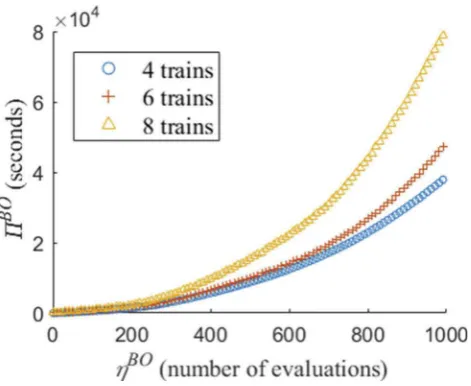
3.5.2. Algorithm computation time

To investigate the relationship betweenηBO_{and the algorithm time of BO,}BO_{,Figure 4}

displays the measured total computation time for the bayesopt algorithm at varying iterations with different numbers of trains. The computation time required was found to be insensitive to the number of carriages so this is not displayed. For each task the data plotted is the median from eight repeat experiments.Figure 4shows that the computa-tional cost of thebayesopt implementation grows rapidly at later iterations of the algo-rithm. This is thought to be specific to the use of a GP model within BO and the associated matrix inversion, rather than inherent to the BO approach. The data also shows that the algorithm computation time increases faster for tasks with more trains. This is because increasing the number of trains in the task increases the GP model matrix dimensions and the associated cost of inverting it. Taking the logarithm ofBO andηBO, to determine the order of computational cost as a function ofηBO_,Oηb

, givesb¼2:73 . However, testing to larger values ofηBO _{would be required to confirm thatbis not larger.}

4. Discussion

The results in Figure 2 show that for all the test-tasks, the BO implementation finds acceptable solutions in significantly less objective function evaluations than the GA. It is not expected that this is unique to the test-tasks. However, the results in Figure 3 indicate that increasing the target performance of the solution leads to an at least exponential increase in the number of objective evaluations required by BO. This is thought to be because in general, for jobs with a high target performance, a proxy function which accurately models the objective function is required. This demands a higher density of evaluations but when many evaluations become clustered in one

region the ability of BO to effectively select new candidates is reduced [29]. In addition to the increase in objective function evaluations, the results in Figure 4 indicate that there is a super-linear relationship between the number of evaluations and the algo-rithm cost. This is thought to be because of the matrix inversion when calculating a GP. Both these effects are thought to be a consequence of implementing BO with a GP model rather than inherent in the BO method. Investigating the effect of using a different probabilistic model within the BO is an area for future investigation.

The results indicate that for certain tasks BO may find ‘good’ solutions in signifi -cantly fewer objective function evaluations than a GA. For tasks involving expensive-to-compute objective functions, this leads to a reduction in total computational expense. When a GP regression model is used as the probabilistic model within BO, increasing the quality of the solution required significantly increases this total expense. However if accelerated techniques for calculating GP models, such as the one developed by Gardner et al. [24], can be implemented with the BO method, this effect might be reduced. The threshold solution quality and computational cost of one evaluation (γ) for which BO is cheaper than GA, are task specific. As identified by McLeod et al. [29] it is likely that in applications where the target performance for the solution is high, a multi-strategy optimization method would be most effective, that is switching from BO to GA (or another alternative).

5. Conclusions

evaluate the suitability of BO for the optimization of expensive-to-compute transporta-tion network models, investigatransporta-tion of a wider range of tasks (e.g. train scheduling or driving tasks) and a greater number of optimization variables is a target for the next stages of research in this area.

Nomenclature

fð Þx A general objective function μð Þx A proxy function

σð Þx An uncertainty function αð Þx An acquisition function

Fðx;λ;θÞ A specific objective function x Solution vector

x Candidate vector

n Number of optimization variables in a task λ Fixed network parameters

θ Passenger load

m Number of carriages to be allocated

R Number of trains

L Number of lines

S Number of line speed choices

F _{Target performance of solution}

η Number of objective function evaluations used

γ One objective function evaluation computational cost (seconds) Γ Evaluating the objective function computational cost seconds)

Algorithm computational cost (seconds)

I Number of algorithm iterations

P GA population size

Disclosure statement

No potential conflict of interest was reported by the authors.

Funding

Funding received from Network Rail and EPSRC grant number EP/M508135/1.

ORCID

Bob Hickish http://orcid.org/0000-0003-2526-7863

David I. Fletcher http://orcid.org/0000-0002-1562-4655

Robert F. Harrison http://orcid.org/0000-0002-9323-8637

References

[2] Yao X, Zhao P, Qiao K. Simulation and evaluation of urban rail transit network based on multi-agent approach. J Ind Eng Manage.2013;6(1):367–379.

[3] Landex A, Nielsen OA. Simulation of disturbances and modelling of expected train passenger delays. In: Allan J, Brebbia CA, Rumsey AF, editors. Computers in railways X. Southampton (UK): WIT Press;2006. p. 85–93.

[4] Kanai S, Shiina K, Harada S, et al. An optimal delay management algorithm from passengers’ viewpoints considering the whole railway network. J Rail Transp Plan Manage.2011;1(1):25–37.

[5] Wei L, Yuan ZZ. A robust timetabling model for a metro line with passenger activity information. Inf.2017;8(3):102–122.

[6] Xu XM, Li KP, Li X. A multi-objective subway timetable optimization approach with minimum passenger time and energy consumption. J Adv Transp.2016;50(1):69–95. [7] Goodwin JCJ, Fletcher DI, Harrison RF. Multi-train trajectory optimisation to maximise

rail network energy efficiency under travel-time constraints. Proc Inst Mech Eng F Rail Rapid Transit.2016;230(4):1318–1335.

[8] Fan B, Roberts C, Weston P. A comparison of algorithms for minimising delay costs in disturbed railway traffic scenarios. J Rail Transp Plan Manage.2012;2(1):23–33.

[9] Estimates of Station Usage 2016–2017 [Internet]. London (UK): Office of Rail and Road;

2017 [cited 2018 Nov 7]. Available from: http://orr.gov.uk/__data/assets/pdf_file/0020/ 26129/estimates-of-station-usage-2016-17-key-facts.pdf

[10] Snoek J, Larochelle H, Adams RP. Practical Bayesian optimization of machine learning algorithms. In: Pereia F, Burges CJC, Bottou L, et al., editors. Proceedings of the 25th International Conference on Neural Information Processing Systems; 2012 Dec 3; Lake Tahoe (NV). New York (USA): Curran Associates; 2012. p. 2951–2959.

[11] Jordan MI, Mitchell TM. Machine learning: trends, perspectives, and prospects. Science.

2015;349(6245):255–260.

[12] Candelieri A, Perego R, Archetti F. Bayesian optimization of pump operations in water distribution systems. J Glob Optim.2018;71(1):213–235.

[13] Lisicki M, Lubitz W, Taylor GW. Optimal design and operation of Archimedes screw turbines using Bayesian optimization. Appl Energy.2016;183:1404–1417.

[14] Schultz L, Sokolov V. Bayesian optimization for transportation simulators. Procedia Comput Sci.2018;130:973–978.

[15] Trotter M, Liu GY, Wood T. Into the storm: descrying optimal configurations using genetic algorithms and Bayesian optimization. In: Frantz CK, Iannucci S, Pitt J, editors. IEEE 2nd International Workshops on Foundations and Applications of Self* Systems; 2017 Sep 18; Tucson (AZ). Washington (DC): IEEE Computer Society Conference Publishing Services; 2017. p. 175–180.

[16] Chandrashekaran A, Lane I Automated Optimization of decoder hyper-parameters for online LVCSR. In: Cardinal P, Hansen JHL, editors. IEEE Workshop on Spoken Language Technology; 2016 Dec 13; San Diego (CA). [Washington (DC)]: IEEE; 2016. p. 454–460.

[17] Goldberg DE. Genetic algorithms in search, optimization, and machine learning. Reading (MA): Addison-Wesley;1989.

[18] Mitchell M. An introduction to genetic algorithms. Cambridge, (MA): MIT Press;1996. [19] Shahriari B, Swersky K, Wang Z, et al. Taking the human out of the loop: A review of

Bayesian optimization. Proce IEEE.2016;104(1):148–175.

[20] Kandasamy K, Schneider J, Piczos B. High dimensional Bayesian optimisation and bandits via additive models. In: Bach F, Beli D, editors. Proceedings of the 32nd International Conference on Machine Learning; 2015 Jul 6; [Lille (France)]: JMLR; 2015. p. 295–304.

Intelligence; 2017 Aug 19; Melbourne (Australia). [place unknown]: International Joint Conferences on Artificial Intelligence Organization; 2017. p. 2096–2102.

[22] Li JJ, Ranka S, Sahni S. Strassen’s matrix multiplication on GPUs. In: Mutka M, Shieh CK, Cheng ST, et al., editors. 17th IEEE International Conference on Parallel and Distributed Systems; Tainan, Taiwan: IEEE; 2011 Dec 7; Washington (DC): IEEE Computer Society Conference Publishing Services;2011. p. 157–164.

[23] Ballard G, Benson AR, Druinsky A, et al. Improving the numerical stability of fast matrix multiplication. SIAM J Matrix Anal Appl.2016;37(4):1382–1418.

[24] Gardner J, Pleiss G, Weinberger KQ, et al. GPyTorch: blackbox matrix-matrix Gaussian process inference with GPU acceleration. In: Bengio S, Wallach H, Larochelle H, et al., editors. Neural Information Processing Systems 2018; Montreal, Canada: Neural Information Processing Systems Foundation; 2018.

[25] Abbink E, van Den Berg B, Kroon L, et al. Allocation of railway rolling stock for passenger trains. Transp Sci.2004;38(1):33–41.

[26] Railway Upgrade Plan 2017/2018 [Internet]. London (UK): Network Rail;2018[cited 2018 Nov 7]. Available from: https://cdn.networkrail.co.uk/wp-content/uploads/2017/08/ Railway-Upgrade-Plan-Update-2017-2018.pdf

[27] Hickish B, Fletcher DI, Harrison RF. Maximising passenger satisfaction through optimised train movements. In: How F, Iwnicki S, Odetunde S, et al., editors. The Stephenson Conference; 2017 Apr 25–27; London (UK): The Institution of Mechanical Engineers; 2017. p. 181–192.

[28] Chambers J, Cleveland W, Kleiner B, et al. Comparing data distributions. In: Chambers J, editor. Graphical methods for data analysis. Belmont (CA): Wadsworth International Group;1983. p. 62–63.

[29] McLeod M, Osborne M, Roberts S. Optimization, fast and slow: optimally switching between local and Bayesian optimization. In: Dy J, Krause A, editors. Proceedings of the 35th International Conference on Machine Learning; 2018 Jul 10; Stockholm (Sweden). [place unknown]: PMLR; 2018. p. 3443–3452.

Appendix

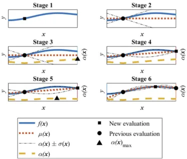
Figure 5.Illustration of six of the early stages in the BO approach. The objective function,fð Þ, is_x shown by a solid line, the proxy function,μð Þ, is shown by a dotted line and the uncertainty aboutx

the proxy function,μð Þ x σð Þ, is shown by a dash-dot line. The values ofx fð Þ,x μð Þx andμð Þ x σð Þx

are plotted on the left ordinate. The acquisition function,αð Þ, is shown by a dashed line and itsx