Model-based inflation forecasts and monetary policy rules. NBB Working Paper Nr. 1

N A T I O N A L B A N K O F B E L G I U M

WORKING PAPERS - RESEARCH SERIES

MODEL-BASED INFLATION FORECASTS AND

MONETARY POLICY RULES

_______________________________

Raf Wouters(*) Michel Dombrecht(*)

The views expressed in this paper are those of the authors and do not necessarily reflect the views of the National Bank of Belgium.

The authors would like to thank Philippe Moës for his helpful comments. The paper was presented at the colloquium on "Optimal Monetary Policy Rules and Accountability" University of Antwerp (UFSIA) on May 10th, 1999.

(*)

Editorial Director

Jan Smets, Member of the Board of Directors of the National Bank of Belgium

Statement of purpose:

The purpose of these working papers is to promote the circulation of research results (Research Series) and analytical studies (Documents Series) made within the National Bank of Belgium or presented by outside economists in seminars, conferences and colloquia organised by the Bank. The aim is thereby to provide a platform for discussion. The opinions are strictly those of the authors and do not necessarily reflect the views of the National Bank of Belgium.

The Working Papers are available on the website of the Bank:

http://www.nbb.be

Individual copies are also available on request to:

NATIONAL BANK OF BELGIUM

Documentation Service boulevard de Berlaimont 14 B - 1000 Brussels

Imprint: Responsibility according to the Belgian law: Jean Hilgers, Member of the Board of Directors, National Bank of Belgium. Copyright © National Bank of Belgium

Reproduction for educational and non-commercial purposes is permitted provided that the source is acknowledged.

Abstract

In this paper, the interaction between inflation and monetary policy rules is

analysed within the framework of a dynamic general equilibrium model derived from

optimising behaviour and rational expectations. Using model simulations, it is illustrated

that the control of monetary policy over the inflation process is strongly dependent on the

role of forward looking expectations in the price and wage setting process and on the

credibility of monetary policy in the expectation formation process of the private sector.

Furthermore, the central bank should take into account a wide variety of indicators in

making monetary policy decisions in order to approach the optimal monetary policy rule as

TABLE OF CONTENTS:

1. INTRODUCTION ...1

2. A DYNAMIC GENERAL EQUILIBRIUM MODEL FOR AN OPEN ECONOMY...4

2.1. Technologies and firms...5

2.1.1. Final-good sector...5

2.1.2. Intermediate goods producers...6

2.1.3. Capital rental firms ...9

2.2. The household sector ...10

2.3. The government sector ...13

2.4. The balance of payments and foreign demand ...13

2.5. Market equilibrium...14

2.6. The parameterisation of the model ...15

3. SIMULATION RESULTS ...18

3.1. Illustration of the impact of the monetary policy rule on the inflation forecast ...19

3.2. Difference between accommodating and non-accommodating monetary policies ...20

3.3. Illustration of the importance of rigidity in the inflation process ...21

3.4. Illustration of the credibility issue for monetary policy...22

3.5. Illustration of the importance of the information that is included in the monetary policy reaction function ...23

4. CONCLUSION ...26

1. INTRODUCTION

Inflation forecasts depend on the expected monetary policy behaviour, at least if

central bank actions have some effect on inflation over the forecast horizon. Model-based

inflation forecasts will therefore depend on the maintained hypothesis about future

monetary actions in the simulation exercise. Empirical studies have illustrated that this

central bank behaviour can be approximated by relatively simple monetary policy rules that

describe systematic relations between the monetary policy instrument, in practice the

short-term interest rate, and some measure of inflation and/or output developments in the

economy1.

If the central bank inflation objective is perfectly credible, the forecast of inflation

over the horizon over which the central bank has control will equal the central bank's

inflation target that is present in the monetary policy rule. But this control is not perfect, for

various reasons. For instance, the cost of bringing down inflation quickly can be too high,

given that the central bank also cares about the real economy. Furthermore, monetary

policy objectives are not always considered as perfectly credible by the public. Such

arguments explain why inflation can deviate from the objective even over a relatively

longer time horizon.

In this paper a small structural model is proposed which is able to explain the

inflation process and its major interactions with other macro-economic aggregates and

which makes it possible to illustrate the role of monetary policy rules in making inflation

forecasts. A model needs to fulfil certain conditions in order to be able to discuss and

compare different monetary policy rules. Ireland (1997) and Rotemberg and Woodford

(1998) argue that structural models derived from optimising behaviour based on rational

(or model-consistent) expectations are robust to the Lucas critique and therefore make it

possible to compare and evaluate alternative monetary policy rules.

The model, calibrated for the euro area, enables us to discuss the impact of

monetary policy rules on inflation forecasts. The importance of monetary policy rules for

model-based forecasts is illustrated by comparing the outcome of a demand shock on

inflation and broader macro-economic aggregates under different monetary policy

reactions.

But the model also enables us to discuss other issues related to the interaction

between the inflation process and monetary policy behaviour in the context of model

simulations. A first topic is the relative importance of lagged inflation versus forward

looking inflation expectations in the price and wage dynamics. Optimising models derived

from the Calvo model or from quadratic adjustment costs2 result in inflation equations that

are purely forward looking. The traditional Taylor nominal-contract model also results in a

purely forward looking inflation equation. This specification has important implications for

monetary policy: it makes disinflation costless if the announced inflation targets are

regarded as credible by the public. This result conflicts with empirical evidence on the cost

of disinflation3. This type of inflation equation is also criticised for not explaining observed

persistence in inflation4. However, the relative importance of lagged versus forward

looking terms in the inflation equations remains an empirical debate. Gali and Gertler

(1998), for instance, found a dominant weight for the forward looking term using the

marginal cost, instead of the traditional output gap, as an explanatory variable in the

inflation equation. In the calibration of our model, a general dynamic specification for both

price and wage inflation is specified and the implications for model simulations and the

sacrifice ratio, in particular, are presented.

A crucial hypothesis in simulations with model-consistent expectations is the

credibility of monetary policy rules and inflation targets in the perception of the private

sector5. This assumption strongly supports the power of monetary policy over inflation

expectations and indirectly over actual price and wage setting. The impact of the perfect

credibility hypothesis is pointed out by comparing the simulation results of a demand shock

under perfect credibility of the monetary policy reaction and inflation target with an

alternative scenario in which the public perceives an incorrect inflation target and only

gradually learns the actual inflation target of monetary policy. The experiment with our

model confirms that the credibility assumption has important effects on the inflation

outcome and that credibility is particularly valuable for central banks as it greatly reduces

the sacrifice ratio of combating inflationary tendencies.

2

See Rotemberg (1996), Hairault and Portier (1993).

3 _{See Ball (1993) for a discussion of the costs of disinflation policies.}

4 _{See Fuhrer and Moore (1995) for evidence on inflation persistence within the framework of contracting models.} 5

A third issue in the relation between monetary policy rules and the inflation

process is the question of whether monetary policy should react to inflation or whether

monetary policy should also consider other macro-economic indicators in making policy

decisions. Svensson's (1998) argument for "inflation forecast" targeting implies that the

central bank should use all relevant information in evaluating and deciding on policy

actions. In the literature, this issue of "optimal monetary rules" is often discussed using a

loss function containing the variance of inflation and output6. Such exercises, based on

stochastic simulations, seek to arrive at a complete model estimate and identification of the

major shocks that drive the economy. In this paper, the topic of "optimal" or

"information-efficient" rules is simply illustrated by pointing to the consequences of different instrument

rules for the sacrifice ratio.

6

2. A DYNAMIC GENERAL EQUILIBRIUM MODEL FOR AN OPEN ECONOMY

The model is an application of the real business cycle methodology for an open

economy with sticky prices and wages7. Households maximise a utility function over a

finite life horizon with the following arguments: consumption of domestic and foreign

goods, money and leisure. Consumption appears in the utility function relative to the

time-varying external habit variable8. Labour is differentiated over households, so that

there is some monopoly power over wages which results in an explicit wage equation and

allows for the introduction of sticky nominal wages à la Calvo. Households allocate wealth

among money, equity, domestic and foreign assets, which are considered as perfect

substitutes, so that UIRP applies in the linear approximation. Firms produce differentiated

goods and decide on labour, capital (with capital adjustment costs), capacity utilisation9

and prices, again according to the Calvo model. Prices are therefore set in function of

current and expected marginal costs. These marginal costs depend on the marginal unit

labour cost (average over the economy) and on the price of imported intermediate inputs,

described further in the text as energy inputs, which are used in fixed proportions in the

production process. The composite domestic good is an imperfect substitute for the

foreign good, so that the real exchange rate is not constant over time.

The model is calibrated on the euro area economy as far as the economic

structure is concerned, while other behavioural parameters are set at realistic values found

elsewhere in the literature. The linear approximation is solved using the forward simulator

available in the Troll software.

Models that are based on dynamic micro-economic foundations for

macro-economic relations are now becoming the standard tool for analysing monetary

policy questions10. The specific model specification, presented in this paper, makes it

possible to discuss various topics: the open economy problem (total versus domestic

inflation), energy or broader commodity price shocks (either as intermediate input in the

production process or as final demand component in consumption), and wage versus price

stickiness (against the one-price models, which do not explicitly incorporate the wage

7

This model is a version of the model considered in Kollman (1997,1998) and features monopolistic competition in both the goods and labour markets.

8 _{Habit depends on lagged aggregate consumption which is unaffected by any one agent's decisions. Abel calls this the} "catching up with the Joneses" effect. See Abel (1990,1996) and Campbell (1998).

9

Following the approach of King and Rebelo (1998). 10

formation process in the labour market)11. In this paper the interaction between inflation

and output behaviour under different monetary policy rules is discussed. On the following

pages we present a brief description of the main building blocks of the model.

2.1. Technologies and firms

The country produces a single final good and a continuum of intermediate goods

indexed by j where j is distributed over the unit interval (j∈

[ ]

perfectly competitive and uses as inputs domestic and imported intermediate goods. The

final good is used for consumption by the representative household and the government

and for investment by the firms that rent out capital. There is monopolistic competition in

the markets for intermediate goods: each intermediate good is produced by a single firm.

2.1.1. Final-good sector

The final good is produced using domestic and imported intermediate goods in

the following CES technology:

(1)

( )

( )

) 1 ( ) 1 /( 1 F t ) 1 /( 1 H t

t y y

Y

γ + γ + γ

+

  

 ₊

=

where γ is a parameter and yH_t and yF_t are indices of domestic and imported intermediate

goods. yH_t can be written as:

(2)

( )

υ + υ +

    

   =

∫

1 1

0

) 1 /( 1 H

j , t H

t y dj

y

where υ is a parameter, and yH_t,j denotes the quantity of domestic intermediate good of

type j that is used in final goods production, at date t.

The cost minimisation conditions in the final goods sector can be written as:

(3) H_t 1 H t H t , j H t , j y p p y υ υ + −        

= and

(4) _t 1 t H t H t Y P p y γ γ + −     =

where pH_j,t is the price of the home intermediate good j , pH_t is the price of the domestically

produced composite intermediate good and P_t is the price of the final good. Perfect

competition in the final goods market implies that the latter two can be written as:

(5)

( )

υ − υ −         =

∫

t p dj

p

(6)

( )

( )

γ − γ − γ −     ₊

= _F 1/

t t / 1 H t

t p sp

P

where s_tis the nominal exchange rate and pF_t is the foreign-currency price of the

composite imported good.

2.1.2. Intermediate goods producers

Each intermediate good

j

j

technology:

(7) y_j,t ≤(1+i_e)AKα_j,tH1_j,−_tα,

where y_j,t (1+i_e) is the firm’s value added, A is a productivity parameter, K_j,t is the

effective utilisation of the capital stock (the distinction between the utilisation rate and the

physical capital stock is discussed in connection with capital rental firms) and H_j,t is an

index of different types of labour used by the firm. This index is given by:

(8) φ + φ + τ         τ =

∫

,j h d

where φ is a parameter and h_j,τ,t is the quantity of type τ labour used by firm j at time t. Energy is used in a fixed proportion, i_e, of value added.

Cost minimisation implies:

(9) _j,t

/ ) 1 ( t t , t , , j H W w h φ φ + − τ

τ =  and

(10) α α − =1 K R H W t , j t t , j t

where R_t is the rental rate of capital, w_τ,t is the wage rate for type τ labour and W_t is an aggregate wage index, given by:

(11)

( )

φ − φ − τ         τ =

∫

t w d

W .

Equation (10) implies that the capital-labour ratio will be identical across intermediate

goods producers and equal to the aggregate capital-labour ratio.

As the production function exhibits constant returns to scale, the firm’s average

and marginal cost are equal and given by:

(12) e e e t t ) 1 ( t 1 t e e e t t H t e t e e e t t K t e t t t i 1 i p s ) ) 1 ( ( R W A 1 i 1 i p s F ) i 1 ( W i 1 i p s F ) i 1 ( R AC MC + + α − α = + + + = + + + = = α − − α − α α −

where F_tK and F_tH are respectively the marginal value added of capital and labour and pe_t

is the foreign-currency price of energy. This implies that the marginal cost, too, is

independent of the intermediate good produced.

Total demand for firm j ’s good equals the sum of domestic and foreign demand:

(13) y_,jt = yH_j,t +xH_j,t,

(14) H_t 1 H t H t , j H t , j x p p x υ υ + −         = ,

and xH_t is aggregate world demand for the country’s exports.

Using equations (3), (13) and (14), nominal profits of firm

j

(15)

(

)

1 H t H t ,j t H t ,j t

,j y x

p p ) MC p ( +         − = π υ υ + −

Each firm j has market power in the market for its own good and maximises

expected profits using a discount rate (βρ_t) which is consistent with the pricing kernel for

nominal returns used by the country’s shareholders-households:

k t C t C k t k t P 1 V V + + + =

ρ , where

C t

V is the marginal utility of consumption at time t (see section 2.2).

The model of price determination, inspired by Calvo (1983), assumes that firms

are not allowed to change their prices unless they receive a random “price-change signal”.

The probability that a given price can be changed in any particular period is constant

(1−ς ) and determines the fraction of all prices that are changed in each period. A producer who is “allowed” to set a new price at time t will maximise the following

intertemporal profit function:

(16) _{t k t k}

0 k

t k k

E _{+ +}

∞ = π ρ β ς

∑

Profit maximisation implies the following mark-up equation:

(17)

( )

( )

∑

∑

Equation (17) shows that the price set by firm

j

are perfectly flexible (ς =0), the mark-up will be constant and equal to 1+υ. With sticky

prices the mark-up becomes variable over time when the economy is hit by exogenous

shocks. A positive demand shock lowers the mark-up and stimulates employment,

investment and real output. Through this last channel the model acquires a Keynesian

character.

The definition of the price index in equation (5) implies that its law of motion is

given by:

(18)

( )

( )

( )

Finally, using equations (3), (7), (10), (13) and (14) the aggregate demand for

capital is given by:

(19) υ υ + − α −         α − α + = =

∫

K ,

where p_tH is determined by the following law of motion:

(18')

( )

( )

( )

υ + − υ υ + − − υ υ + − ς − + ς

= H 1

t , j 1 H 1 t 1 H

t p (1 )p

p

2.1.3. Capital rental firms

Capital is a homogenous factor of production that is owned by firms that rent

capital to producers of intermediate goods. These firms can choose between physical

capital accumulation (Kp) or a higher utilisation rate (z) with K=zKp. Capital accumulation is

given by:

(20)

(

)

[

( )

]

p t 2 p t p 1 t p 1

t K 1 z I

K K K 2

K ₊ +ψ + − = −τ + ,

where ψ is an adjustment-cost parameter, I_t is gross investment and τ

( )

depreciation rate, which is an increasing function of the utilisation rate.

(21)

∑

giving rise to the following first-order condition for capital:

(22)             + τ − βρ = + + + + + + + 1 t 1 t 1 t 1 t 1 t 1 t 1 t t t p R z ) z ( Q p E Q ,

where Tobin’s Q is given by:

(23) p t p t p 1 t t K K K 1

Q = +ψ + −

The first order condition for the utilisation rate equates the cost of higher utilisation in terms

of faster replacement investments with the rental price of capital services.

(24) R_t =p_tτ_z

( )

2.2. The household sector

There is a continuum of households indicated by index

τ

over the supply of its labour. Each household

τ

(25)        

= τ τ _τ

τ t , t t t t t , P M , CH C V V l

Utility depends on consumption of goods, Cτ_t, relative to the external habit variable, CH_t , real cash balances, M_tτ/P_t and labour supply l_τ,t. Households act as price-setters in the labour market.

Household τ’s intertemporal utility function is given by:

(26)

∑

t pr V

E ,

Households hold money balances M_t, domestic government bonds B_t, foreign

interest-bearing bonds F_t and domestic equity U_t. Bonds are one-period bonds with price

t

b for domestic bonds and f_t for foreign bonds. A perfect insurance market inherits

consumers' wealth contingent on their death and redistributes wealth in the form of an

annuity payment in proportion to household wealth. The budget constraint faced by the

household is then given by:

(27)         − − + + + + = + + + τ τ τ τ τ − τ − τ − τ − τ τ τ τ t t t , t t , t 1 t t t 1 t t t 1 t t 1 t t t t t t t t t t t t t T C P w P U d P F s P B P M * ) pr 1 ( P U d P F f s P B b P M l

where d_t represents the capital income return and T_t lump-sum taxes.

Households maximise the objective function (26) subject to the intertemporal

budget constraint (27) and the demand for their labour given in equation (9). As in the

goods market, we assume that wages can only be changed after some random

“wage-change signal” is received. The probability that a particular household can “wage-change its

nominal wage in period t is constant and equal to 1−ξ. A household τ which receives

such a signal in period t, will thus set a new nominal wage w_τ taking into account the probability that it remains unchanged in the future.

This maximisation yields the following first-order conditions for consumption,

wealth allocation and wage-setting, where λ_t is the Lagrange multiplier, i_t is the nominal

rate of return on domestic bonds (1+i_t =1b_t ) and iF_t is the foreign-currency rate of return

on foreign bonds (1+iF_t =1f_t):

(28) V_tc =λ_t/pr

(29) t t t P / M t 1 t 1 t t P P V P

E _+ = λ

(30) t t t 1 t 1 t t p ) i 1 ( p

E _= λ

     + λ β + + (31) t t F t t 1 t 1 t 1 t t p ) i 1 ( s s p

E _ = λ

     + λ β + + + (32) t t t 1 t 1 t 1 t t P d d P

E _ = λ

    λ β + + + (33) i t C i t 0 i i t 1 i t i i t 0 i i t i t 1 i t i i t t , P V H W E ) V ( H W E ) 1 ( w + + ∞ = + φ φ + + ∞ = + + φ φ + + τ

∑

∑

Combining equations (28) and (30) gives the usual first-order condition for

consumption growth. Equations (28), (29) and (30) together result in a money demand

equation. Real money holdings depend on consumption, with an elasticity that is possibly

smaller than one, and the velocity of money depends positively on the interest rate.

Equations (30) and (31) give the uncovered interest rate parity condition for nominal

exchange rate determination. Equation (32) shows that the expected holding return on

equity equals the expected one-period interest rate under certainty equivalence.

Finally, equation (33) shows that the nominal wage at time t of a household

τ

working is a mark-up over the present value of marginal cost (the subjective cost of

working)12. When wages are perfectly flexible (ξ=0), the real wage will be constant

mark-up over the ratio of the marginal disutility of labour and the marginal utility of an additional

unit of consumption.

12

Given equation (11), the law of motion of the aggregate wage index is given by:

(34)

( )

(

)

( )

2.3. The government sector

For the sake of completeness and in order to arrive at a realistic representation of

the final demand components, we also introduce a government sector. The government

has to satisfy the following budget restriction:

(35) _{t t}

t 1 t

t t

t _{G T}

P B P B b − + = − _,

which states that the primary deficit, G−T, and the debt service has to be financed by the

issuing of new public debt B_t at the current price b_t. To rule out explosive debt dynamics,

the following endogenous tax behaviour is assumed:

(36) _

            − = ° P B P B g T t t t ,

where the reaction coefficient g is greater than the real interest rate (g>i−π). This

ensures a stable public debt at the long-term objective Bo.

2.4. The balance of payments and foreign demand

The accumulation of foreign assets F_t is determined by the current account

relation: (37) _t t e t t F t t F t t H t t H t t 1 t t t t t t _IE P p s y P p s x P p P F s P F f s − − + = −

The net foreign asset position depends on the interest payments on existing net foreign

exports, XH_t , and the real value of imports of final goods, Y_tF, and energy inputs,IE_t.

Energy acts only as an input in the production process:

(38) _t

e e

t y

i 1

i IE

+ =

The demand for exports is a function of the terms of trade (s_tpF_t /pH_t ) and demand

in the rest of the world (ROW_t):

(39) _t

F t t

H t H

t ROW

p s

p x

ϑ −

    =

2.5. Market equilibrium

The final goods market is in equilibrium if production equals demand by

consumers, the government and the capital accumulation firms:

(40) Y_t =C_t +G_t +I_t

The capital rental market is in equilibrium when the demand for capital by the

intermediate goods producers equals the supply by the capital rental firms. The labour

market is in equilibrium if firms’ demand for labour equals labour supply at the wage level

set by households. Aggregate consumption behaviour deviates from the first-order

condition describing optimal decisions at household level by the additional wealth effect

resulting from the finite horizon assumption. The external habit variableCH_t is a simple

function of the lagged aggregate consumption level:

(41) CH_t =Ch_t−1

The interest rate is determined by a reaction function that describes monetary policy

decisions. This rule will be discussed in the following sections of the paper. In order to

maintain money market equilibrium, the money supply adjusts endogenously to meet the

In the capital market, equilibrium means that the government debt is held by

domestic investors at the market interest rate i_t (assuming that the country is in a net

foreign asset position), and that the net foreign assets are held by investors at the going

interest and exchange rates.

2.6. The parameterisation of the model

In the standard simulation of the theoretical model the following values for the

coefficients are assumed. The share of capital is set at 0.35 and the parameter for the

cost of capital adjustment is 10. The parameter determining the marginal cost of higher

capacity utilisation (King and Rebelo (1998)) is set at 0.1. In the utility function, we set the

coefficient of relative risk aversion at 1. The habit variable moves with consumption

lagged one period with a coefficient equal to 0.8. The macro-economic labour supply

elasticity with respect to real wages is 0.5.

The structure of final demand is given by the following steady-state assumptions:

final import/gdp = 0.06, energy import/gdp = 0.04, export/gdp = 0.10, consumption/gdp =

0.58, investment/gdp = 0.22, government expenditures/gdp = 0.20, public debt/gdp = 2.4

(60% on annual basis) and net foreign assets/gdp = 0.4 (10% on annual basis). The

discount factor β is set at 0.99, the rate of depreciation is 0.02 and capital/gdp ratio is 11.0.

The import and export price elasticity is set at 0.75. These parameters reflect the

economic structure of a large open economy such as the euro area.

The parameters of the price and wage adjustment equation require further

attention. In the theoretical model we assumed a forward looking inflation specification for

the whole economy. In the simulation of the model we use a generalisation in which the

inflation process is influenced by both forward looking expectations and lagged adjustment

effects13. Following the approach of Tinsley (1993), we assume some general dynamic

13

adjustment cost mechanism in estimating the price and wage dynamics. Price and wage

setters are assumed to minimise the following cost of adjustment expression:

(42)

(

)

(

)

(

)

     ∆ + − + − β ₊ = − + + + + ∞ =

∑

∑

i _{b p p b p p b p}

where p* represents the equilibrium price level. This problem results in a general dynamic

expression for inflation:

(43)

( )

(

)

( )

(

)

0 i i j t k 1 j j * 1 t 1

t p b p ,b,k p

p 1 A p ₊ ∞ = − = −

− − + γ ∆ + ϕ β ∆

− =

∆

∑

∑

where A(L)=1+a₁

( )

( )

( )

the lagged variables assumes a value of 0.7, while for the wage dynamics the lagged

variables have a coefficient equalling 0.5514. The impact of the forward looking

expectations is therefore greatly reduced compared to the pure Calvo-price mechanism.

The model specification implies that a monetary shock has persistent effects on

output and inflation. These results contrast with the results of other sticky-price general

equilibrium models15. The difference is explained by some typical characteristics of our

model:

- the introduction of both sticky prices and sticky wages slows down the adjustment

speed of the price system16. Furthermore, the introduction of lagged inflation

terms resulting from the assumed adjustment lags in both price and wage

relations prevents the domestic inflation process from following the typical jump

profile of models with only forward looking expectations17. In our specification the

inflation process will show a gradual and "hump-shaped" response to nominal and

real shocks;

14

The sum of lagged and lead terms is restricted to one in the estimate. 15 _{See Andersen (1998) and Jeanne (1998) for a discussion of this problem.} 16 _{See Erceg (1997).}

17

- a second reason for the persistence of the effects results from the assumption

underlying aggregate demand behaviour. The introduction of habit formation in

the consumption process implies that aggregate demand reacts more smoothly to

shocks18. A slower reaction of output also moderates the reaction of marginal

costs and therefore of prices;

- the introduction of a variable capacity utilisation reduces the short-run impact of

output fluctuations on marginal costs. Higher output in the short run is produced

with a more intensive use of production capacity, so that marginal productivity of

labour declines less strongly and employment moves only slightly more than

proportionally to production. The fact that marginal costs behave in a less volatile

manner also implies that the effect on domestic inflation is somewhat smoothed

over time.

18

3. SIMULATION RESULTS

The role of monetary policy rules in the prediction of inflation based on structural

model simulation is illustrated by analysing the consequences of an exogenous demand

shock on economic activity and the inflation process. Aggregate demand increases

following a shock in government expenditures of one per cent of GDP. The impact of the

shock will depend on the reaction function or the monetary policy rule that describes the

interest rate decisions of the central bank. After an illustration of the impact of the

monetary policy rule on the model simulation outcomes, other aspects of the relationship

between the inflation process and the monetary policy rules are discussed. In the first

place, it is shown that the control exerted by the monetary policy over the inflation rate will

depend on the dynamic properties of the inflation process, the credibility of the monetary

policy and the form of the instrument rule of the central bank. To illustrate the role of these

arguments in the interaction between monetary policy and inflation, the sacrifice ratio, the

output-cost of monetary policy actions necessary to bring inflation down by one per cent, is

used to summarise the outcomes19. This output cost is essentially a short-term cost

related to the gradual adjustment of the inflation expectations following a positive demand

shock. The stabilisation of inflation at a low level will increase long term economic welfare

through different channels20: the reduction in the economy-wide mark-up which will bring

the economy closer to a competitive economy, the reduction in the relative price dispersion

between individual producers reduces welfare costs from misallocation in aggregate

demand, the reduction of the inflation tax on money balances. Inflation may have more

negative effects through mechanisms that fall outside the scope of this paper: the

interaction with a legal and contractual framework that is not adapted to coping with

inflation, uncertainty and volatility of the inflation process disturbing intertemporal and

static allocation problems. In both scenarios economic activity will return towards its

long-term equilibrium growth path. According to the vertical long-long-term Phillips-curve theory, this

level will be independent of the temporal deviation between actual and steady state output.

But the latter may increase if the long-term growth path depends negatively on the average

rate of inflation (the positive Phillips-curve relation between inflation and unemployment).

19

In the literature different monetary policy rules are often compared using the outcome of the loss function, a combination of inflation and output variability, in stochastic simulations. See for instance Haldane and Batini (1998), Svensson (1998), Rotemberg and Woodford (1997).

20

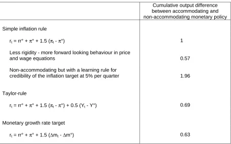
3.1. Illustration of the impact of the monetary policy rule on the inflation forecast

Figure 1 summarises the impact of the exogenous demand shock on inflation and

economic activity as it is simulated with the model. In this scenario, the central bank is

assumed to follow a very simple instrument rule: the interest rate is increased (decreased)

every time that inflation increases (decreases) above its target rate:

(44) r_t =rr° +∆pa +a

(

)

where rr° represents the equilibrium real interest rate and ∆pa the inflation objective of the

central bank. This instrument rule and the inflation objective are announced and are

considered by the market participants as a perfectly credible policy, so that the interest

rate equation becomes part of the model structure and is used as such by the public when

forming model-consistent expectations. In the simulation described in Figure 1, the

coefficient "a" is set at 1.5: the real interest rate increases by 50 basis points if inflation

increases by 1%.

The outcome in Figure 1 shows that the inflation rate will temporally increase

above the target level of the monetary authorities, but the reaction of the central bank will

force inflation back to its target level after some time. As economic activity increases, the

marginal cost of production will increase through different mechanisms: marginal

productivity tends to decrease as the output gap narrows and capacity utilisation

increases, whereas wages will come under upward pressure as unemployment decreases

and expected inflation rises. Higher production costs and the willingness of firms to

restore the mark-up will tend to increase the inflationary pressure in the economy.

Inflation does increase smoothly over time, as the dynamics of price and wage

inflation are influenced by both a backward and a forward looking component. The

backward looking terms in the inflation equations prevent inflation from jumping

immediately to a higher level, thereafter possibly returning gradually to the target rate.

This behaviour results from the existence of contracts and other rigidities in the price and

wage setting that limit the flexibility of the inflation dynamics. The lead terms in the

inflation equations result from the forward looking behaviour: price and wage setters who

can change their price at a certain moment will take into account the expected cost

increases in the future when deciding on the new price level, as its price is likely to remain

will be influenced by the monetary policy rule and the inflation target. The monetary policy

actions provide the nominal anchor on which market participants can base their

expectations. Depending on the monetary policy rule, expectations regarding future

inflation developments will differ and the outcome of the actual price and wage decisions

will also differ. If the central bank reacts strongly to inflation movements and keeps clearly

to the previously announced inflation target, market expectations regarding future inflation

will be very moderate, so that the inflation process does not gain momentum. Firms will be

motivated to restrict cost increases and will therefore be reluctant to increase supply or

output levels. Higher real interest rates and real appreciation of the exchange rate

decrease aggregate demand. Inflation and output will return relatively quickly to the

equilibrium growth path.

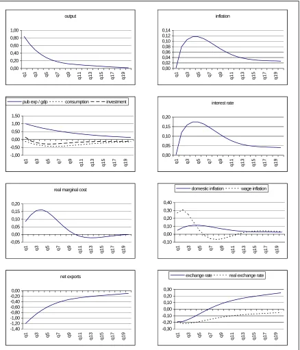
Figure 2 shows that for a less strong reaction of the central bank to the demand

shock (for example when, in the reaction function, the coefficient for inflation "a" is reduced

from 1.5 to 1.25), inflation will increase more strongly and more persistently. In this

scenario the expansion of output will also be greater. Both inflation and output-gap

variance increase in this scenario. In a more extreme case, where the coefficient for

inflation is smaller than 1, this means that the real interest rate will decrease following the

increase in inflation, the model will not produce a unique solution, and any inflation path

becomes possible21. The central bank fails to provide a nominal anchor under such a

monetary policy rule22. Prediction of the future inflation path becomes impossible as any

outcome can result from self-fulfilling expectations.

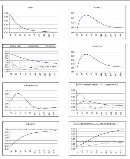
3.2. Difference between accommodating and non-accommodating monetary policies

Figure 3 summarises the results of a simulation in which the central bank reacts

accommodatingly to the inflationary pressure resulting from the increase in economic

activity. In this scenario the central bank adjusts the inflation objective upwards in order to

support economic activity following an expansion in demand. For instance, let us assume

that the central bank increases the inflation objective by one per cent following an increase

in demand emanating from public expenditures. Here it is assumed that the higher

inflation objective is announced and taken into account by market participants when doing

their planning and especially when setting their prices and wages.

21 _{See Bernanke and Woodford (1997) and Clarida, Gali and Gertler (1998).}

These results should be compared to the results in Figure 1 describing the

non-accommodating monetary policy reaction following the demand shock. It is clear that the

total area below the output curve is larger under the accommodating monetary policy. This

means that the non-accommodating monetary policy has a clear temporal cost in terms of

output. This cost is called the sacrifice ratio in the economic literature23. The sacrifice

ratio is here defined as the cumulative output cost of bringing down inflation by one

percentage point in the non-accommodating scenario compared to the accommodating

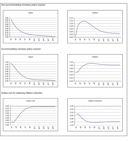
scenario (see Table 1 and Figure 3b).

3.3. Illustration of the importance of rigidity in the inflation process

The long-term price-wage behaviour is determined by fundamental economic

determinants (productivity, inflation objective, goods and labour market characteristics,

etc.). But the dynamic behaviour is strongly dependent on adjustment lags and

expectations about the future. Adjustment lags are largely explained by the existence of

contracts and other market rigidities due to market regulation, monopoly situations, or just

behaviour by simple rules of thumb.

The relative weight of forward versus backward looking elements in the dynamic

price and wage behaviour are crucial for the speed and the cost at which the central bank

can influence the inflation process. In the baseline model the dynamic processes for

prices and wages were based on estimation results from a general dynamic

cost-of-adjustment model for the euro area. In these estimation results the relative weight of

forward expectations in the price-setting process was relatively limited (30%) versus (70%)

for the lagged price dynamics. For the nominal wage equations the relative importance

was estimated at (45%) forward versus (55%) backward.

It is clear that with a 100% forward looking model, monetary policy would have an

immediate and costless control over the inflation process if the central bank were fully

credible. In such a situation it would be sufficient to announce a lower inflation target to

have an immediate impact on the actual inflation rate. If, however, there are adjustment

lags or backward looking effects in the inflation process, the adjustment will take more time

and it will cause a short-term cost. To illustrate the importance of these relative weights

23

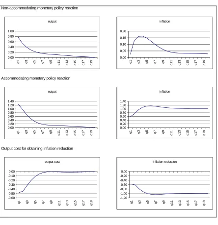
we simulate an alternative model in which the relative weight of the forward looking

expectations has been increased by 10% for both prices (40%) and wages (55%).

Repeating the exercise of a demand shock with an accommodating and a

non-accommodating monetary policy allows us to calculate again the sacrifice ratio, or in other

words the total output costs incurred to obtain a reduction in the inflation rate of 1%. With

fewer market rigidities, contracts or other mechanisms causing backward looking elements

in the price - wage process, the cost of reducing inflation is substantially lower (see Table

1 and Figure 4). Market expectations have a stronger impact on the actual price and wage

setting, so that, under the perfect credibility assumption, the impact of monetary policy

announcements will have a stronger impact on actual price movements. This reduces the

need for real interest rate increases and the corresponding output effects in the inflation

reduction process.

3.4. Illustration of the credibility issue for monetary policy

The price and wage dynamics not only depend on the importance of market

rigidities but also on the credibility of monetary policy in the perception of the market

participants. In the previous examples, monetary policy was very powerful in influencing

the expectations of market participants because of the assumption of perfect credibility.

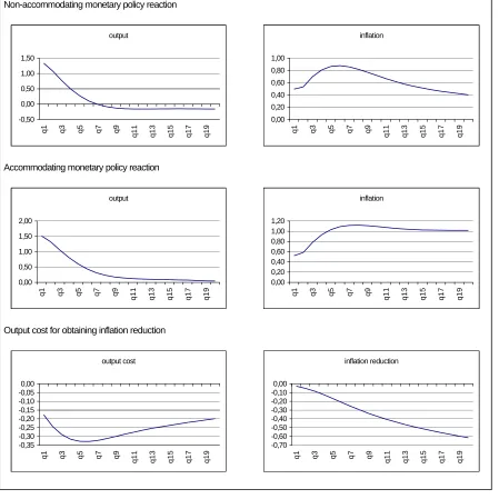
To illustrate the role of the credibility issue, we make an alternative simulation in which the

central bank announcement only gradually (over time) affects the expectations of market

participants regarding future price and wage developments. The rate at which the market

adapts its expectations towards the newly announced target is fixed deterministically at 5%

per quarter. Thus the inflation target perceived by the public ∆pp_t gradually moves

towards the correct inflation target that determines monetary policy actions ∆pa:

(45) ∆pp_t =0.95∆pp_t−1+0.05∆pa

In the previous simulations, full credibility was assumed through the model

consistent expectations formation process. As the central bank's monetary policy rule was

part of the model structure, the market participants used the announced monetary rule and

inflation objective in making their predictions about future variables relevant for actual

However, market participants may not believe that the central bank will adhere to

its monetary policy rule or to the announced inflation objective. To illustrate this problem,

we assume that market participants believe that the central bank will react

accommodatingly to a demand shock, so that output and inflation can increase strongly.

The central bank will actually adhere to the constant inflation target and increase the

interest rate according to the previously announced rule and objective. Market participants

observe "unexpected" interest rate shocks, and will “learn” only gradually over time that the

central bank has kept its original inflation target. In the example we assume a speed of 5%

per quarter. In the meantime the central bank has however shocked the economy, by a

series of unexpected interest rate increases, so that the output effects will be smaller than

in the accommodating case. The output cost of reducing inflation to the original inflation

level will in this case be considerably higher than with the perfect credible

non-accommodating policy.

Table 1 and figure 5 show that the sacrifice ratio is considerably higher under the

"learning" assumption. The cost of reducing inflation by one per cent, calculated as the

difference in cumulative output difference under the accommodating and the

non-accommodating policy is much higher than in the perfect credibility simulation results. The

role of expectations in the disinflation process is limited in this scenario, so that the central

bank has to make more use of its interest rate (and exchange rate) instruments to fight the

inflation process.

3.5. Illustration of the importance of the information that is included in the monetary policy reaction function

In the previous simulations it was assumed that the central bank used a very

simple instrument rule to determine its policy actions. The central bank increases the

interest rate each time inflation surpasses the target inflation rate. Such a simple

instrument rule will in general not be optimal for the central bank. Even if the objective

function of the central bank includes inflation variability as its only objective, the optimal

behaviour of the central bank will be more complex than just a simple relation between the

interest-rate instrument and the inflation-target variables.

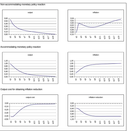
An alternative instrument rule is for instance the Taylor rule, that is considered in

empirical research as a good approximation to the actual monetary policy behaviour both

of the Federal Reserve in the US (Taylor (1993)) and for European countries, such as the

strategy the central bank will increase its interest rate if inflation increases above the

inflation target (the real interest rate will rise by 0.5 points for a 1% increase in inflation) but

also if the output level increases above its equilibrium or potential output level (the real

interest rate will rise by 0.5 points for a 1% reduction in the output gap).

(46) r_t =rr° +∆pa +a

(

) (

)

Using the Taylor-reaction function instead of the simple inflation-reaction rule, we

can repeat the simulation experiment with an accommodating and a non-accommodating

reaction to a demand shock and recalculate the sacrifice ratio. The sacrifice ratio under

the more general Taylor rule turns out to be smaller compared to the simpler reaction

function (see Table 1 and Figure 6) .

The interpretation of this result is that the central bank uses more information to

decide on its monetary policy actions under the Taylor rule. By incorporating information

on the stance of the output gap in its decisions, the central bank not only looks at the

actual inflation figures, but also at future inflation pressure that is present in the observed

output-gap value. The result is that the central bank will react more strongly immediately

following the appearance of the demand shock, but that it will reverse its policy more

quickly once the output effects of the shock disappear. Using this rule means that

monetary policy results in a soft-landing scenario following an expansive demand shock,

preventing excessively strong fluctuations in output and inflation.

This result also indicates that there is an important difference between the

ultimate objective of monetary policy on the one hand and the reaction function or

instrument rule on the other hand. Although the objective can be defined narrowly in terms

of inflation targeting, the central bank should take a larger set of economic variables into

account in reaching its monetary policy decisions.

This example can be considerd as an illustration of the more general principle that

the central bank should use a broad area of indicators for deciding on its monetary policy

actions. In these circumstances monetary policy can approach the optimal monetary

policy which allows the ultimate target to be approximated at minimum cost. One has

therefore to determine the optimal weights in the reaction function with respect to the

different indicators. Under such an optimal rule, the impacts of monetary actions are

model this problem is complicated, as the monetary policy has a direct inflation effect via

the exchange rate channel and a slower, longer-term effect via the interest rate channel.

This profile does not necessarily correspond to the inflationary impact of a demand shock.

Thus the central bank has to use all available information for predicting the future course of

inflation and the impact of its policy actions before deciding on the optimal policy reaction.

The policy should however remain clear and understandable to the public.

Without fulfilment of this condition, a large part of the monetary policy effect, through its

impact on market expectations, will be lost. This balancing of arguments summarises the

difficult problems facing central banks in their decisions on monetary policy and in

communicating the policy to the public. The money aggregate can play a role in this

process, as it incorporates information on both the inflation gap (deviation of actual versus

optimal target inflation), the output gap and the velocity gap (excess liquidity in the

system)24. Using a monetary growth rate targeting rule25, the same simulation experiment

shows that the sacrifice ratio can be further decreased, compared to the simple inflation

rule or Taylor rule for monetary policy (see Table 1)26. Of course such a result disregards

the possible problems caused by velocity instability.

24 _{See Coenen (1998) on the comparison of inflation and monetary targeting in a P-star model.}

25 _{Consumption was replaced by total output, with unit elasticity, in the money-demand equation for this exercise.} 26

4. CONCLUSION

In this paper, the interaction between inflation and monetary policy rules is

analysed within the framework of a structural model derived from optimising behaviour and

rational expectations. Using model simulations, it is shown that the control exercised by

monetary policy over the inflation process is strongly dependent on the role of forward

looking expectations in the price and wage setting process and on the credibility of

monetary policy in the expectation formation process of the private sector. Furthermore,

the central bank should take into account a wide variety of indicators in making monetary

policy decisions, in order to approach the optimal monetary policy rule as closely as

possible. However such complications should not conflict with the public's understanding

of the monetary policy behaviour. Therefore, clear communication of the monetary

strategy and presentation of the arguments supporting it are crucial conditions for efficient

central bank behaviour.

The understanding of the transmission mechanism and the price and wage

inflation process are important ingredients in the monetary decision process. Further

elaboration of dynamic general equilibrium models can help in analysing these

mechanisms and show their dependency on the monetary policy behaviour. Especially the

theoretical derivation of dynamic price-wage inflation equations and the empirical

estimation of these models are necessary steps in this process. The resulting

identification of the stochastic shocks makes it possible to carry out stochastic simulation

exercises. The optimal monetary policy can then be derived explicitly by using an

objective function for central bank behaviour. Such exercises should include the

Table 1 - Indices of sacrifice ratios under different monetary policy and model assumptions (Annual basis, sacrifice ratio of first reported result is set equal to 1)

Cumulative output difference between accommodating and non-accommodating monetary policy

Simple inflation rule

rt = rr° + π° + 1.5 (πt - π°) 1

Less rigidity - more forward looking behaviour in price

and wage equations 0.57

Non-accommodating but with a learning rule for

credibility of the inflation target at 5% per quarter 1.96

Taylor-rule

rt = rr° + π° + 1.5 (πt - π°) + 0.5 (Yt - Y°) 0.69

Monetary growth rate target

Figure 1 - Impulse-response of a demand shock (public expenditures)

under a non-accommodating monetary policy following a simple inflation instrument rule rt = rr° + π° + 1.5 (πt - π°)

output

0,00 0,20 0,40 0,60 0,80 1,00

q1 q3 q5 q7 q9 _{q11 q13 q15 q17 q19}

inflation

0,00 0,02 0,04 0,06 0,08 0,10 0,12 0,14

q1 q3 q5 q7 q9 _{q11 q13 q15 q17 q19}

-1,00 -0,50 0,00 0,50 1,00 1,50

q1 q3 q5 q7 q9 _{q11 q13 q15 q17 q19}

pub exp / gdp consumption investment interest rate

0,00 0,05 0,10 0,15 0,20

q1 q3 q5 q7 q9 _{q11 q13 q15 q17 q19}

net exports

-1,40 -1,20 -1,00 -0,80 -0,60 -0,40 -0,20 0,00

q1 q3 q5 q7 q9

q11 q13 q15 q17 q19

-0,30 -0,20 -0,10 0,00 0,10 0,20 0,30

q1 q3 q5 q7 q9

q11 q13 q15 q17 q19

exchange rate real exchange rate real marginal cost

-0,05 0,00 0,05 0,10 0,15 0,20

q1 q3 q5 q7 q9

q11 q13 q15 q17 q19

-0,10 0,00 0,10 0,20 0,30 0,40

q1 q3 q5 q7 q9

q11 q13 q15 q17 q19

Figure 2 - Impulse-response function of a demand shock (public expenditures) under a non-accommodating monetary policy following a simple inflation instrument rule

rt = rr° + π° + 1.25 (πt - π°)

output

0,00 0,20 0,40 0,60 0,80 1,00

q1 q3 q5 q7 q9

q11 q13 q15 q17 q19

inflation

0,00 0,05 0,10 0,15 0,20

q1 q3 q5 q7 q9

q11 q13 q15 q17 q19

-0,60 -0,40 -0,20 0,00 0,20 0,40 0,60 0,80 1,00 1,20

q1 q3 q5 q7 q9

q11 q13 q15 q17 q19

pub exp / gdp consumption investment _{interest rate}

0,00 0,05 0,10 0,15 0,20 0,25

q1 q3 q5 q7 q9

q11 q13 q15 q17 q19

net exports

-1,40 -1,20 -1,00 -0,80 -0,60 -0,40 -0,20 0,00

q1 q3 q5 q7 q9

q11 q13 q15 q17 q19

-0,30 -0,20 -0,10 0,00 0,10 0,20 0,30 0,40 0,50

q1 q3 q5 q7 q9

q11 q13 q15 q17 q19

exchange rate real exchange rate real marginal cost

-0,05 0,00 0,05 0,10 0,15 0,20 0,25

q1 q3 q5 q7 q9

q11 q13 q15 q17 q19

-0,10 0,00 0,10 0,20 0,30 0,40 0,50

q1 q3 q5 q7 q9

q11 q13 q15 q17 q19

Figure 3 - Impulse-response function of a demand shock (public expenditures) under an accommodating monetary policy following a simple inflation instrument rule

rt = rr° + π° + 1.5 (πt - π°) and π° increases by 1%

output 0,00 0,20 0,40 0,60 0,80 1,00 1,20 1,40 1,60

q1 q3 q5 q7 q9 _{q11 q13 q15 q17 q19}

inflation 0,00 0,20 0,40 0,60 0,80 1,00 1,20

q1 q3 q5 q7 q9

q11 q13 q15 q17 q19

-1,00 -0,50 0,00 0,50 1,00 1,50 2,00 2,50

q1 q3 q5 q7 q9

q11 q13 q15 q17 q19

pub exp / gdp consumption investment _{interest rate}

0,00 0,20 0,40 0,60 0,80 1,00 1,20 1,40

q1 q3 q5 q7 q9

q11 q13 q15 q17 q19

net exports -0,60 -0,40 -0,20 0,00 0,20 0,40 0,60 0,80 1,00

q1 q3 q5 q7 q9 _{q11 q13 q15 q17 q19}

0,00 1,00 2,00 3,00 4,00 5,00 6,00

q1 q3 q5 q7 q9 _{q11 q13 q15 q17 q19}

exchange rate real exchange rate real marginal cost

-0,10 0,00 0,10 0,20 0,30 0,40 0,50 0,60 0,70

q1 q3 q5 q7 q9

q11 q13 q15 q17 q19

0,00 0,20 0,40 0,60 0,80 1,00 1,20 1,40 1,60

q1 q3 q5 q7 q9 _{q11 q13 q15 q17 q19}

Figure 3b - Impulse-response function of a demand shock (public expenditures) under an accommodating monetary policy following a simple inflation instrument rule

rt = rr° + π° + 1.5 (πt - π°) and π° increases by 1%

Non-accommodating monetary policy reaction

Accommodating monetary policy reaction

Output cost for obtaining inflation reduction output

0,00 0,20 0,40 0,60 0,80 1,00 1,20 1,40 1,60

q1 q3 q5 q7 q9 _{q11 q13 q15 q17 q19}

inflation

0,00 0,20 0,40 0,60 0,80 1,00 1,20

q1 q3 q5 q7 q9 _{q11 q13 q15 q17 q19}

output

0,00 0,10 0,20 0,30 0,40 0,50 0,60 0,70 0,80 0,90

q1 q3 q5 q7 q9 _{q11 q13 q15 q17 q19}

inflation

0,00 0,02 0,04 0,06 0,08 0,10 0,12 0,14

q1 q3 q5 q7 q9 _{q11 q13 q15 q17 q19}

output cost

-0,80 -0,70 -0,60 -0,50 -0,40 -0,30 -0,20 -0,10 0,00

q1 q3 q5 q7 q9 _{q11 q13 q15 q17 q19}

inflation reduction

-1,20 -1,00 -0,80 -0,60 -0,40 -0,20 0,00

Figure 4 - Impulse-response function of a demand shock (public expenditures) under a simple inflation instrument rule in a model with less rigidity

in the price and wage equation

Non-accommodating monetary policy reaction

Accommodating monetary policy reaction

Output cost for obtaining inflation reduction

output

0,00 0,20 0,40 0,60 0,80 1,00

q1 q3 q5 q7 q9

q11 q13 q15 q17 q19

inflation

0,00 0,05 0,10 0,15 0,20

q1 q3 q5 q7 q9

q11 q13 q15 q17 q19

output

0,00 0,20 0,40 0,60 0,80 1,00 1,20 1,40

q1 q3 q5 q7 q9

q11 q13 q15 q17 q19

inflation

0,00 0,20 0,40 0,60 0,80 1,00 1,20 1,40

q1 q3 q5 q7 q9

q11 q13 q15 q17 q19

output cost

-0,60 -0,50 -0,40 -0,30 -0,20 -0,10 0,00

q1 q3 q5 q7 q9

q11 q13 q15 q17 q19

inflation reduction

-1,20 -1,00 -0,80 -0,60 -0,40 -0,20 0,00

q1 q3 q5 q7 q9

Figure 5 - Impulse-response function of a demand shock (public expenditures) under a non accommodating monetary policy following a simple inflation instrument rule

where the announced objectives is only gradually perceived as credible by the public (5% learning rule)

Non-accommodating monetary policy reaction

Accommodating monetary policy reaction

Output cost for obtaining inflation reduction

output

-0,50 0,00 0,50 1,00 1,50

q1 q3 q5 q7 q9 _{q11 q13 q15 q17 q19}

inflation

0,00 0,20 0,40 0,60 0,80 1,00

q1 q3 q5 q7 q9 _{q11 q13 q15 q17 q19}

output

0,00 0,50 1,00 1,50 2,00

q1 q3 q5 q7 q9 _{q11 q13 q15 q17 q19}

inflation

0,00 0,20 0,40 0,60 0,80 1,00 1,20

q1 q3 q5 q7 q9 _{q11 q13 q15 q17 q19}

output cost

-0,35 -0,30 -0,25 -0,20 -0,15 -0,10 -0,05 0,00

q1 q3 q5 q7 q9

q11 q13 q15 q17 q19

inflation reduction

-0,70 -0,60 -0,50 -0,40 -0,30 -0,20 -0,10 0,00

q1 q3 q5 q7 q9

Figure 6 - Impulse-response function of a demand shock (public expenditures) under Taylor-rule for monetary policy

rt = rr° + π° + 1.5 (πt - π°) + 0.5 (Yt - Y°)

Non-accommodating monetary policy reaction

Accommodating monetary policy reaction

Output cost for obtaining inflation reduction

output

0,00 0,10 0,20 0,30 0,40 0,50 0,60

q1 q3 q5 q7 q9

q11 q13 q15 q17 q19

inflation

-0,10 -0,08 -0,06 -0,04 -0,02 0,00 0,02 0,04

q1 q3 q5 q7 q9

q11 q13 q15 q17 q19

output

0,00 0,20 0,40 0,60 0,80 1,00 1,20

q1 q3 q5 q7 q9 _{q11 q13 q15 q17 q19}

inflation

0,00 0,20 0,40 0,60 0,80 1,00 1,20

q1 q3 q5 q7 q9 _{q11 q13 q15 q17 q19}

output cost

-0,50 -0,40 -0,30 -0,20 -0,10 0,00

q1 q3 q5 q7 q9

q11 q13 q15 q17 q19

inflation reduction

-1,20 -1,00 -0,80 -0,60 -0,40 -0,20 0,00

q1 q3 q5 q7 q9

References

Andersen, T.M. (1998), "Persistency in sticky price models", European Economic Review , No. 3-5 (May), pp. 593-603.

Aucremanne, L. and Wouters, R. (1999), "A structural VAR approach to core inflation and its relevance for monetary policy", in BIS (ed.), Measures of underlying inflation and their role in the conduct of monetary policy - proceedings of the workshop of central bank model builders held at the BIS on 18-19 February 1999, Bank of International Settlements, Basel, Switzerland.

Ball, L. (1993), “What determines the sacrifice ratio?”, NBER Working Papers, No. 4306.

Bernanke, B. and Woodford, M. (1997), “Inflation forecasts and monetary policy”, NBER Working Papers, No. 6157.

Blake, A.P. and Westaway, P.F. (1996), “Credibility and the effectiveness of inflation targeting regimes", The Manchester School Supplement, pp. 28-50..

Blanchard, O. (1985), “Debt, deficits, and finite horizons”, Journal of Political Economy, 93(2), pp. 223-247.

Bomfin, A., Tetlow, R., von zur Muehlen, P. and Williams, J. (1997), “Expectations, learning and the costs of disinflation: experiments using the FRB/US Model", BIS Conference Papers, 1997.

Campbell, J. (1998), "Asset prices, consumption, and the business cycle", NBER Working Papers, No. 6485.

Calvo, G. (1983), “Staggered prices in a utility maximising framework”, Journal of Monetary Economics, 12, pp. 383-398.

Chari, V.V., P.J. Kehoe, and E.R. McGratten (1996), “Monetary shocks and real exchange rates in sticky price models of international business cycles”, NBER Working Paper, No. 5876.

Christiano, L.J., Eichenbaum M. and Evans C.L. (1997), "Sticky prices and limited participation models of money: a comparison", European Economic Review, No. 6 (June), pp.1201-1249.

Clarida, R., Gali, J. and Gertler, M. (1997), "Monetary policy rules in practice: some international evidence", NBER Working Paper, No. 6254.

Clarida, R., Gali, J. and Gertler, M. (1998), "Monetary policy rules and macroeconomic stability: evidence and some theory", CEPR Discussion Paper, No. 1908.