Inversion of Surface Deformation Data for Rapid Estimates
of Source Parameters and Uncertainties: A Bayesian Approach
Marco Bagnardi1,2 and Andrew Hooper1
1
COMET, School of Earth and Environment, University of Leeds, Leeds, UK,2Now at Jet Propulsion Laboratory, California Institute of Technology, Pasadena, CA, USA
Abstract
New satellite missions (e.g., the European Space Agency’s Sentinel-1 constellation), advances in data downlinking, and rapid product generation now provide us with the ability to access space-geodetic data within hours of their acquisition. To truly take advantage of this opportunity, we need to be able to interpret geodetic data in a prompt and robust manner. Here we present a Bayesian approach for the inversion of multiple geodetic data sets that allows a rapid characterization of posterior probability density functions (PDFs) of source model parameters. The inversion algorithm efficiently samples posterior PDFs through a Markov chain Monte Carlo method, incorporating the Metropolis-Hastings algorithm, with automatic step size selection. We apply our approach to synthetic geodetic data simulating deformation of magmatic origin and demonstrate its ability to retrieve known source parameters. We also apply the inversion algorithm to interferometric synthetic aperture radar data measuring co-seismic displacements for a thrust-faulting earthquake (2015Mw6.4 Pishan earthquake, China) and retrieve optimal source parametersand associated uncertainties. Given its robustness and rapidity in estimating deformation source parameters and uncertainties, our Bayesian framework is capable of taking advantage of real-time geodetic
measurements. Thus, our approach can be applied to geodetic data to study magmatic, tectonic, and other geophysical processes, especially in rapid-response operational settings (e.g., volcano observatories). Our algorithm is fully implemented in a MATLAB®-based software package (Geodetic Bayesian Inversion Software) that we make freely available to the scientific community.
1. Introduction
Geodetic observational data, most commonly global navigation satellite system (GNSS) and interferometric synthetic aperture radar (InSAR) measurements, are regularly used to infer information about sources of sur-face displacements and to understand the underlying processes. With these aims, inverse problem theory has been applied to geodetic data to study magmatic systems (Pinel et al., 2014, and references therein), the earthquake cycle (Elliott et al., 2016, and references therein), and many other geophysical phenomena that cause deformation of the Earth’s interior and surface such as the response to ice load changes, changes in aquifer storage, and geothermal exploitation (e.g., Auriac et al., 2014; Juncu et al., 2017; Samsonov et al., 2014). However, many commonly employed inversion approaches aim at solely determining an optimal set of source parameters—for example, the weighted least-squares“best-fitting”model—by solving an opti-mization problem that minimizes the weighted misfit between measured and simulated surface displace-ments. Among these, the most commonly used methods are simulated annealing (e.g., Cervelli et al., 2001) and genetic algorithm (e.g., Currenti et al., 2005). These have shown to be successful in solving a variety of optimization problems to study different geophysical problems (Sambridge & Mosegaard, 2002), and a detailed analysis of these methodologies, applied to the inversion of InSAR data, is presented by Shirzaei and Walter (2009). Direct-search methods (e.g., simulated annealing and genetic algorithm) do not fully and appropriately characterize uncertainties associated with the source parameter estimates, with the risk that results can be inadequately interpreted. In fact, it is common that a wide range of model parameter values can adequately explain the observations, and it is therefore fundamental to know the credible interval of such values, especially if interpretations are used for the assessment and mitigation of natural hazards or in operational settings (e.g., volcano observatories).
The application of a Bayesian approach when inverting geodetic data (e.g., Anderson & Segall, 2013; Fukuda & Johnson, 2010; Hooper et al., 2013; Jolivet et al., 2015; Minson et al., 2013) allows the characterization of posterior probability density functions (PDFs) of source parameters, which are formulated by taking into
RESEARCH ARTICLE
10.1029/2018GC007585
Key Points:
• We present a Bayesian approach for the inversion of geodetic data and demonstrate successful applications to synthetic and real data
• Our approach allows rapid estimates of source parameters and uncertainties and is well suited for rapid-response and operational settings
• We have implemented our approach in a MATLAB®-based software package (GBIS) that is made freely available to the scientific community
Correspondence to:
M. Bagnardi,
Citation:
Bagnardi, M., & Hooper, A. (2018). Inversion of surface deformation data for rapid estimates of source parameters and uncertainties: A Bayesian approach. Geochemistry, Geophysics, Geosystems, 19, 2194–2211. https://doi.org/10.1029/ 2018GC007585
Received 30 MAR 2018 Accepted 14 JUN 2018
Accepted article online 27 JUN 2018 Published online 27 JUL 2018
©2018. The Authors.
account uncertainties in the data (e.g., data errors and incompleteness) and any available prior information (in the form of a prior PDF). The Bayesian method provides the means to investigate a wealth of statistical inferences, such as point estimates (e.g., mean and median of posterior distributions), credible intervals (e.g., quantiles), and direct probability statements about parameters (e.g., the probability that a certain parameter is greater than a certain value). It also allows analyses of joint and conditional probabilities of pairs or sets of parameters and is particularly instructive in the case of non-Gaussian multimodal posterior PDFs. An optimal set of source parameters can also be extracted from the posterior PDF byfinding the maximum a posteriori probability solution.
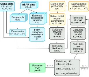
In this work we propose an approach, summarized in Figure 1, for inverting geodetic data—in particular those derived from InSAR measurements—using a Bayesian probabilistic inversion algorithm capable of including multiple independent data sets (e.g., González et al., 2015; Hooper et al., 2013; Sigmundsson et al., 2014). To efficiently sample the posterior PDFs, we implement a Markov chain Monte Carlo method (MCMC), incorporating the Metropolis-Hastings algorithm (e.g., Hastings, 1970; Mosegaard & Tarantola, 1995), with automatic step size selection. We then review and discuss existing methodologies to characterize errors in InSAR data and to subsample large data sets, which are both necessary steps to be performed prior to an inversion. The proposed method is applied to the inversion of synthetic InSAR and GNSS data to demonstrate the ability of the algorithm to retrieve known source parameters. Finally, as a test case, we invert InSAR data spanning the 2015Mw6.4 Pishan (China) earthquake and determine the fault model parameters
for this blind thrusting event and validate our results through the comparison with other independent stu-dies (e.g., Ainscoe et al., 2017; He et al., 2016; Wen et al., 2016).
[image:2.612.222.530.88.355.2]The proposed approach has been implemented in a software package (Geodetic Bayesian Inversion Software [GBIS], http://comet.nerc.ac.uk/gbis) that we make freely available to the scientific community. The software is written in MATLAB® (which is a commercial software and needs to be installed in order to run GBIS) and uses, among others, analytical forward models from the dMODELS software package (Battaglia et al., 2013). Simple mechanical models of crustal deformation that use closed-form analytical solutions for the character-ization of magmatically or tectonically induced deformation processes (e.g., Lisowski, 2007; Segall, 2010) can
compute surface displacements at 103–105observation points in 103–101s on consumer-grade computers. These models can be used to place constraints on source location, geometry, orientation, and strength (e.g., volume changes in a magma reservoir and slip on a fault), and their rapidity in computing surface displace-ments makes them suitable for exploring large numbers (e.g., 106) of model parameter combinations. Numerical forward models (e.g., boundary elements method) can also be used to explore more complex source geometries or to take into account complexities in the Earth’s crust (e.g., nonflat topographic surface; e.g., Bathke et al., 2015; Cayol & Cornet, 1997; Hooper et al., 2011). However, the increase in complexity in the forward model significantly increases the computational burden, making numerical models less efficient in operational or rapid-response investigations.
Finally, with this work we aim at proposing a detailed guideline for the use of geodetic measurements in inverse problems and present a potential standardized procedure that would allow appropriate comparisons of results obtained by different entities. Inversion results are often used to populate global data sets of defor-mation source models (e.g., Biggs & Pritchard, 2017; Ebmeier et al., 2018) and should therefore be of compar-able quality and obtained with a congruent approach.
2. Bayesian Inversion
For a given discrete inverse problem, the data vectord= {d1,d2,…,dND} is equal to a nonlinear model func-tion,G, of the model parametersm= {m1,m2,…,mNM}, plus errorϵ:
d¼G mð Þ þϵ (1)
In a Bayesian framework, the posterior PDF,p(m|d), describes the probability associated with a given set of model parametersmthat is based on how well such parameters can explain the datadgiven their uncertain-ties, while considering any prior information. The posterior PDF is calculated as follows:
pðmjdÞ ¼pðdjmÞpð Þm
pð Þd (2)
wherep(d|m) is the likelihood function ofmgivendbased on residuals between the data and the model pre-diction of the observations,p(m) expresses the prior information (in the form of a prior joint PDF) of the model parameters, and the denominator is a normalizing constant independent ofm.
When the errors are multivariate Gaussian with zero mean and covariance matrixΣd,ϵ~N(0,Σd), the likeli-hood function is calculated as follows:
pðdjmÞ ¼ð Þ2πN=2j jΣd 1
2exp 1
2ðdGmÞ
T
Σ1
d ðdGmÞ
(3)
whereNis the total number of data points andΣ1
d is the inverse of the variance-covariance matrix for a given
set of data. The data vectordcan be formed from multiple data sets (e.g., multiple SAR interferograms or a combination of interferograms and GNSS data). The likelihood function for multiple data sets, assuming inde-pendence, can therefore be expressed as the product of the likelihoods of the data sets (e.g., Fukuda & Johnson, 2008):
pðdjmÞ ¼∏Kk¼1ð Þ2πNk=2j jΣk 1
2 exp 1
2r
T kΣk1rk
(4)
whereNkis the number of data points andrkare the residual vectors (difference between observed and mod-eled data,rk=dkGkm) associated with eachkth data set andKis the total number of data sets. Similarly,
the prior probability of the model vector, assuming independence for the model parameters, is the product of the prior probabilities of the different model parametersmj:
pð Þ ¼m ∏NMj¼1p mj (5)
When inverting geodetic data to infer model parameters for deformation sources, prior information is often not available, in which case a so-called uninformative Jeffreys prior is used (Jeffreys, 1939; Ulrych et al., 2001). This depends on the universe of possible outcomes and, in cases where all values for a given parameter are equally probable, for example, source location parameters, is simply uniform. If there is afinite range of pos-sible values, upper and lower bounds can be added outside whichp(m) = 0. However, some source para-meters cannot assume negative values (for example, length and width of a rectangular dislocation or the aspect ratio describing a magmatic source) and must be treated accordingly. An appropriate uninformative prior for nonnegative parameters that could equally well be described by the reciprocal of the parameter is a logarithmic prior. In our generalized algorithm, we transform the prior for these cases into a uniform prior, by treating the logarithm of the parameter of interest as the actual model parameter.
Finally, there are other sources of error that are intrinsic to the chosen model (e.g., material properties of the crust) and its ability to accurately predict the data (known as model or prediction errors, e.g., Duputel et al., 2014). While the effect of model/prediction errors should still be considered in any ultimate interpretation (e.g., Jolivet et al., 2015), they are strongly case dependent and difficult to implement in a widely applicable approach. We therefore do not consider model/prediction errors further in this manuscript, as they are also not implemented in the GBIS software.
2.1. Sampling the Posterior Probability With MCMC
An efficient way to sample and therefore characterize a posterior probability distribution is through a MCMC sampling method (Mosegaard & Tarantola, 1995). Using the Metropolis-Hastings algorithm (Hastings, 1970; Metropolis et al., 1953), the sampling can be efficiently controlled so that after a sufficiently large number of iterations, the density of the samples approximates the posterior distribution.
The approach, summarized in Figure 1, starts with the selection of an initial set of model parametersmi =0
from the prior distribution p(m)—either arbitrarily chosen or previously estimated using a direct-search method such as simulated annealing—and the estimation of the associated likelihood functionp(d|mi). A
new trial set of model parameters is generated by taking a random step withinp(m). When the prior for each model parameter is uniform and independent, this is achieved by perturbing each parameter inmiby an
amountanΔmj, whereanis a random value generated from a uniform distribution within the range [1, 1]
andΔmjis the maximum random walk step size for each parametermj. If a model parameter of the new model trial falls outside the bounds of the uniform prior probability, we replace this value,mjTRIAL*, as follows:
mjTRIAL¼2UBjmjTRIAL ifmjTRIAL>UBj
mjTRIAL¼2LBjmjTRIAL ifmjTRIAL<LBj
(
(6)
whereUBjandLBjare the upper and lower bounds, respectively, of the uniform probability for a given model parametermj. The likelihood for the new set of model parametersp(d|mi +1) is then calculated, and if its value is greater than the previous one,p(d|mi +1)>p(d|mi), the step is taken and the trial model values are retained. If the new likelihood value is less than the previous one,p(d|mi +1)<p(d|mi), the step is taken with a probability equal to the ratio of the new likelihood and the previous one, that is, ifp(d|mi +1)/p(d|mi)≥b, wherebis a random value from a uniform distribution within the range [0, 1]. Otherwise the previous set of model parameters is retained by settingmi +1tomi.iis then incremented, and the steps described above are iterated from the selection of a new trial set of model parameters.
This approach guarantees that sets of model parameters that improve the probability of the current model are always retained, while those with lower probability are sometimes retained, allowing the algorithm to escape local minima. The process is repeated until a representative sampling of the posterior distribution is achieved (e.g., 105–107iterations).
2.2. Automatic Step Size Selection
we automatically tune the size ofΔmjfor each model parameter during thefirst 20,000 iterations by perform-ing a sensitivity test everyNsiterations (e.g.,Ns= 100 fori<1,000;Ns= 1,000 for 1,000<i<20,000). In a similar way to Amey et al. (2018), we aim atfindingΔmjsuch that the mean chance of acceptance approaches the optimal acceptance rate of 23.4% (Roberts et al., 1997) and to ensure that all parameters approximately equally contribute to the changes in likelihood. The optimal acceptance/rejection ratios are maintained by monitoring the evolution of the perturbed probability ratio (PPR) for each parameter, defined as the ratio between the current posterior probability and the posterior probability calculated after perturbing the para-meter value by half of the current step size. If the PPR is greater than one, its reciprocal is taken. A target PPR,
PPRTARGET, is set as follows:
PPRTARGET¼
1 2
1 NM
i¼1
PPRTARGET¼ PPRTARGETiNs
RRCURRENT
RROPTIMAL
i>1 8
> > < > > :
(7)
where PPRTARGETi-Nsis the target PPR at the time of the previous sensitivity test,RRCURRENTis the current rejec-tion rate, andRROPTIMALis the optimal rejection rate (76.6%). In this approach, if too many model trials are
rejected, PPRTARGETwill decrease, while if not enough model trials are kept, PPRTARGETwill increase.
The step size for each parameter is then adjusted, with the aim that its PPR approaches PPRTARGET. Such
changes are achieved by adjusting the maximum step size,Δmj, for each model parameter as follows:first, we calculate the PPR and subtract it from PPRTARGET. We define this difference aspDIFF. IfpDIFF<0, which
means that the model parameter’s contribution to the posterior probability change is too large, the step size must be reduced. IfpDIFF>0, the model parameter’s contribution must be increased by increasing the step size. For each case, the step size is adapted as follows:
Δmji¼ΔmjiNsexp pDIFF
PPRTARGET2
ifpDIFF<0
Δmji¼ΔmjiNsexp pDIFF
1PPRTARGET
ifpDIFF>0 8
> > > < > > > :
(8)
After 20,000 iterations, the maximum step size,Δmj, isfixed to that tuned through the sensitivity tests for all remaining iterations. The aim is to achieve, at the end of the inversion, an acceptance rate between 15% and 50% (e.g., Roberts & Rosenthal, 2001).
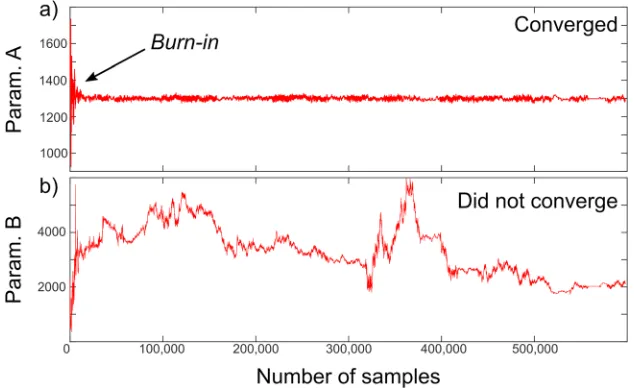
2.3. Estimating Convergence and Burn-in Period
After all iterations have been completed (i=I) and before working on the statistics of posterior PDFs, it is important to check that the Markov chain has converged. If a Markov chain does not converge, it does not explore the parameter space sufficiently, and the sampled posterior distribution does not approximate the target distribution well. Note that the convergence for all parameters should be checked. While there are no exact ways to determine the convergence of a Markov chain, there are empirical tools to evaluate it. For example, the visual examination of the trace plots, which display the accepted values of a parameter as a function of iteration number, can be instructive (Figure 2). Trace plots are also useful to determine the number of early samples that strongly depend on the choice of the starting value, known as the“burn-in” period, during which the MCMC algorithm walks from a highly improbable starting model to models with rea-sonable values ofp(d|m), and starts adequately sampling the posterior PDF. Choosing a burn-in period that is too short may leave unrepresentative samples in the posterior PDF, and since these samples have parameter values that are typically far from those in high posterior probability areas, they may unrealistically increase the credible interval for a given parameter. Conversely, choosing a too large burn-in period will discard repre-sentative samples of the posterior PDF that could instead be used to improve the accuracy of the statistics (e.g., Sahlin, 2011). In Figure 2 we display examples of trace plots showing a chain that has converged after the burn-in period, and one that did not converge.
Anderson & Poland, 2016). This step can also be used to check that PDFs for all chains converge to similar distributions, independently from the chosen initial set of model parameters.
3. Data Errors and Subsampling
3.1. Estimates of Data Errors
The Bayesian approach requires that we quantify errors in the data, which we assume are drawn from a multi-variate Gaussian distribution. We achieve this by estimating the data variance and covariance, for each inde-pendent data set. In our approach, GNSS data are characterized by variances associated to each displacement component, namely,σ2N,σ2E, andσ2V, for the north, east, and vertical components at each site, respectively.
Such values, obtained through standard GNSS data processing (e.g., Herring et al., 2015), populate the diag-onal of the variance-covariance matrixΣd, which has all remaining off-diagonal elements set to 0, assuming
that no covariance exists between the three components of displacement or between individual GNSS mea-surement sites. However, when available, covariance between components can be placed in the variance-covariance matrix accordingly.
Conversely, we directly characterize the errors in InSAR data by experimentally estimating variance and cov-ariance in each independent data set. Together with randomly distributed noise caused by phase decorrela-tion, it is well known that InSAR data are affected by spatially correlated phase delays that are mainly caused by spatiotemporal changes in water vapor content in the atmosphere, known as the“wet”tropospheric delay (e.g., Hanssen et al., 1999). Further spatially correlated errors can be caused by topographic residuals, which are phase change artifacts introduced during data processing. Although errors in InSAR data may sometimes have two-dimensional spatial structures (anisotropy; Knospe & Jónsson, 2010), for simplicity we assume that they are isotropic and stationary (e.g., errors estimated in non-deforming areas are the same as in adjacent deforming areas) and calculate theoretical semivariograms that have the same characteristics as the data (e.g., Lohman & Simons, 2005; Sudhaus & Jónsson, 2009).
A semivariogram measures the spatial variability of a regionalized variable by computing the dissimilarity between pairs of data values (e.g., Wackernagel, 1995). Usually, values at two places near to one another are similar, whereas those at more widely separated distances are less so. By expressing the lag distanceh (Euclidean distance) between two observation pointsxiandxi + hand by averaging increments in equidistant
[image:6.612.216.533.91.286.2]bins, the experimental semivariogrambγð Þh for a quantityQis calculated as follows:
bγð Þ ¼h 1 2N ∑
N
i¼1 ðQ xð iþhÞ–Q xð Þi 2
(9)
whereNis the number of data-point pairs in each distance bin. For second-order stationary processes, the semivariogram and the covariance function are related as follows:
γð Þ ¼h Cð Þ 0 C hð Þ (10)
whereC(0) is the covariance at lag distanceh= 0—i.e., the variance—andC(h) is the covariance at any given distanceh.
For InSAR data, we recommend calculating the experimental semivariogram over an area of the data set of at least the same size as the area subject to surface deformation under investigation and where deformation is also not expected and/or observed. An efficient way to achieve this is to mask deforming areas from the data set and to calculate the semivariogram using all remaining data points (e.g., Figure 3). It is also recommended to remove a linear ramp of the formZ(x,y) =ax+by,whereaandbare linear coefficients of thexandy coor-dinates, respectively, to account for any residual orbital error or very long wavelength atmospheric delay across the entire InSAR data set (e.g., Sudhaus & Jónsson, 2009). The parameters for a linear ramp across an entire image can then be estimated directly from the data during the inversion.
[image:7.612.218.530.87.387.2]In our approach, to keep the problem computationally efficient but still adequately representative of the entire data set, the semivariogram is calculated from 3,000 randomly drawn points over 30 equal distance
Figure 3.(a) Sentinel-1 descending interferogram over southern Isabela Island, Galápagos (Ecuador). Track 128, 24 June 2017 to 06 July 2017. Black arrows show theflight direction of the satellite and the look direction with the incidence angle in degrees. Cerro Azul and Sierra Negra are two active volcanoes. Gray shading covers an area of deformation that should be masked when computing the experimental semivariogram. (b) Experimental (diamonds) and theoretical (solid line) semivariograms computed for the image in panel (a), with the exception of the deforming area. The continuous functionγ(h) is an unbounded exponential one-dimensional function with a nugget, defined in equation (11), with
bins (h= maximum distance between points/30). We successively estimate the least squares bestfit to the experimental semivariogram using an unbounded exponential one-dimensional function with a nugget:
γð Þ ¼h s0þðss0Þ 1–exp h
r
(11)
wheres0is the nugget variance—that is, the variance value as the lag distance approaches 0 and
represent-ing the variability at distances smaller than the sample spacrepresent-ing—sis the sill variance (including the nugget variance), andris the the range (Figure 3). Note that for an unbounded exponential function, where the semi-variogram increases asymptotically toward its sill value, the effective rangerεequals 3rand is the distance at whichγ(h) has increased to 95% of the sill variances. Based on equation (10), the covariance can be calculated for any distance between points as follows:
C hð Þ ¼
s h¼0
s0þðss0Þ exp h r
h>0 8
< :
9 =
; (12)
A large number of theoretical functions can be used tofit the experimental semivariogram and to simulate the covariance in InSAR data (for example, see González & Fernández, 2011, and references therein). Among these models, we chose the unbounded exponential one-dimesional function with nugget because of its simple implementation and ability to well approximate the power law behavior exhibited by the spatial structure of atmospheric delay.
3.2. Subsampling of InSAR Data
InSAR data can provide surface displacement measurements over continuous large areas (for example, a Sentinel-1 wide-swath image product covers an area of ~250 × 180 km2) with over 108measurement points when data are processed at full resolution. The inversion of such large data sets would be therefore extremely computationally expensive, making spatial subsampling a necessary step to achieve a tractable computa-tional burden. Any subsampling approach must, on the other hand, maintain enough information as possible for the inversion to be successful.
Three main types of InSAR data downsampling methods can be applied: uniform sampling (e.g., Pritchard et al., 2002), resolution-based sampling (e.g., Lohman & Simons, 2005; Wang et al., 2014), and gradient-based sampling (e.g., Jonsson, 2002; Simons, 2002). Uniform sampling extracts data at regularly spaced locations across the image, and while it is the simplest approach, it is also the least suitable for an effective sampling of those areas where surface displacements are most diagnostic for estimates of deformation source para-meters. To achieve the appropriate data point density in such areas, this approach often leads to a data vector that is still too large for efficient inversions. Conversely, resolution-based sampling uses the design of the inverse problem to determine the optimal data sampling density and is based on the data resolution matrix, with higher density of points in the nearfield and fewer points in the farfield. This approach, despite being shown to be the best performing in the inversion of InSAR data (Wang et al., 2014), requires some knowledge of the source of deformation itself (e.g., the fault plane geometry) and is therefore not always applicable, especially when the estimation of source location and geometry is the main goal of the inversion. Finally, gradient-based sampling methods increase data point density in those areas characterized by higher displa-cement gradients and vice versa. While this approach may oversample areas where higher displadispla-cement gra-dients are not caused by deformation but by noise (e.g., atmospheric delay or topographic errors), it is the most generally suitable in cases where no prior knowledge on the source geometry and location is available. An appropriate characterization of the data errors (see section 3.1) can also mitigate the effect of oversam-pling noisy areas.
morefinely than areas with low variance (e.g., nondeforming areas, farfield). Once the points within a polygon have variance lower than the selected threshold, the mean value of such points is assigned to a sample point with the coordinates of the centroid of the polygon. This strategy allows for nonsquare, irregularly aligned polygons, which reduce the effect of data gaps within and at the edges of InSAR images, a shortcoming of the“classic”quadtree approach. Small polygons with less than three points are eliminated to avoid sampling in areas with extreme deformation gradients, where these are likely to be inaccurately unwrapped during processing (e.g., very near field, surface rupture of faults). The variance
threshold can be iteratively adjusted until the minimum possible data vector length is achieved while main-taining a sampling sufficiently high to characterize the deformationfield.
After subsampling the InSAR data, the theoretical covariance function estimated using the experimental semivariogram (see section 3.1) is used to populate the variance-covariance matrix according to the distance between the polygon centroids.
4. Validation Using Synthetic GNSS and InSAR Data
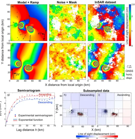
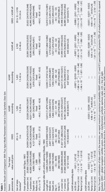
We demonstrate and assess the validity of our Bayesian inversion approach using synthetic deformation data that simulate surface displacements caused by magmatic sources. In this example, we produce two InSAR line-of-sight (LOS) displacement maps, simulating images from a descending and from an ascending pass of the satellite (Figures 4a–4f), and GNSS three-dimensional displacements at 20 sites randomly distributed over the area of interest (black arrows in Figure 4a show the GNSS horizontal components). Surface displace-ments are generated using a set of arbitrarily chosen model parameters (Table 1) and forward models for a deflating finite spherical source (McTigue, 1987) and a rectangular dipping dike with uniform opening (Okada, 1985), assuming an isotropic elastic half-space with Poisson’s ratioν= 0.25.
To make the synthetic data more representative of real measurements, we randomly assign a standard devia-tion to each component of the GNSS data ranging between 1 and 9 mm (the standard deviadevia-tion of the ver-tical component is on averagefive times larger than that of the horizontal components). In the case of InSAR data, wefirst add a linear ramp and a rigid offset in the LOS direction, we then simulate atmospheric noise using an isotropic two-dimensional fractal surface with a power law behavior (Hanssen, 2001), andfinally we remove randomly distributed portions of the data sets to simulate low-coherence areas (Figures 4b and 4e). Synthetic three-dimensional displacements are projected into the LOS direction using uniform inci-dence angles of 41° and 29° and heading angles of 191° and 349° for the descending and ascending data sets, respectively.
We calculate the experimental semivariogram of the added atmospheric noise in each InSAR data set and estimate best-fit exponential functions (Figure 4g) with sill variance sDESC = 4.85 mm2
(s0DESC = 4 × 109 mm2) and a range distance rDESC = 9,380 m for the descending data, and
sASC= 5.42 mm2(s0ASC= 8 × 109mm2) andrASC= 8,350 m for the ascending data. We then apply the
quad-tree subsampling algorithm and retrieve the data vectorsdDESCwith 1,453 data points anddASCwith 1,292 data points (Figures 4h–4i).
The inversion algorithm is tested usingfive data combinations: GNSS data only, the descending InSAR data set, the ascending InSAR data set, both InSAR data sets, andfinally all three data sets (2× InSAR + GNSS). We assume a uniform prior probability for all source parameters (logarithmic for nonnegative parameters) between reasonable bounds and perform 106iterations to sample the posterior PDFs (thefirst 2 × 10⁴ itera-tions are not retained as they represent the burn-in period/step size adjustment). All inversion results are reported in Table 1.
In all cases, the true input model parameters fall between the 2.5 and 97.5 percentiles of the posterior PDFs, which validates our inversion algorithm. As expected, the uncertainty in the model parameters varies as a function of the size of the data vector (e.g., looser when using only GNSS data and tighter for all combinations that use InSAR data) and the errors in the data. The duration of each inversion, when performed on a consumer-grade computer, varies between 3 min (GNSS only) and 3.5 hr (all data).
5. Application to the 2015
M
w6.4 Pishan Earthquake
As a test case, we apply the Bayesian inversion approach to three InSAR data sets spanning the 3 July 2015Mw
(González et al., 2016), which uses routines from the GAMMA InSAR software package to process Sentinel-1 terrain observation by progressive scans SAR data.
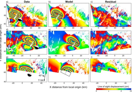
The three Sentinel-1 interferograms show coseismic deformation consistent with thrust faulting on an ENE-WSW striking structure. Ascending interferograms (Figures 5a and 5d) show two lobes with a characteristic “butterfly”shape, where LOS displacements are toward the satellite (a combination of uplift and predomi-nantly northward horizontal motion) northwest of the epicenter and away from the satellite (a combination of subsidence and predominantly southward horizontal motion) west-southwest of the epicenter. The des-cending interferogram (Figure 5g), which only covers the northern portion of the coseismic displacement
field, also shows LOS displacements toward the satellite north of the epicenter. Maximum LOS displacements of ~0.12 m are recorded at the center of the uplifting lobe.
[image:12.612.81.531.89.403.2]Wefirst estimate the experimental semivariogram for deformation-free regions of each InSAR data set andfit the theoretical exponential function (see Table 2). We then subsample the data sets using a variance
Figure 5.(left column) Sentinel-1 terrain observation by progressive scan interferograms for 2015Mw6.4 Pishan earthquake; (middle column) forward model using the maximum a posteriori probability solution; and (right column) residual maps. Black arrows on data plots show theflight direction of the satellite, the look direction with the incidence angle in degrees, and the track number. The beach ball represents the fault plane solution from global centroid moment tensor catalogue and marks the epicentral location. The black rectangle on model plots represents the outline of the optimal fault plane, with the thicker line outlining the updip edge of the fault and the arrow representing the direction of slip. Differential interferograms show coseismic displacements measured between (top row) 30 June 2015 to 24 July 2015, (middle row) 11 June 2015 to 05 July 2015, and (bottom row) 24 June 2015 to 18 July 2015.
Table 2
Details for Interferometric Synthetic Aperture Radar Data Sets Used in the Inversion
Track-pass Sill variance (m2) Nugget variance (m2) Range distance (m) No. of data points
129-ascending 7.6 × 10⁵ 8 × 10⁹ 12,900 310
56-ascending 2.5 × 10⁵ 4 × 10⁹ 15,000 475
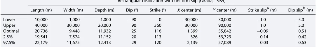
[image:12.612.42.575.686.741.2]threshold of 3 × 10⁵m2and obtain a data vector composed of 1,146 data points (the contribution of each data set is reported in Table 2). The inversion is carried out using a kinematic forward model for a rectangular dislocation source (Okada, 1985) with nine source model parameters: length, width, depth of the lower edge, dip angle (positive upward from horizontal), strike (measured clockwise from north),XandYcoordinates of the midpoint of the lower edge, uniform slip in the strike direction, and uniform slip in the dip direction. We also estimate a rigid shift in the LOS direction since all InSAR measurements are relative to an arbitrary refer-ence point, and the coefficients for a linear ramp,a(x) andb(y), for each interferogram. The model parameter vectormis therefore composed of 18 parameters, for which we assume uniform priors between reasonable bounds (logarithmic for nonnegative parameters; see Table 3). Priors for fault geometry are based on pre-vious results (Ainscoe et al., 2017; He et al., 2016; Wen et al., 2016) and on the size of the measured deforma-tionfield, while no constraints are imposed onto fault strike (varying between 0° and 360°) and dip angles (varying between90° and +90° from horizontal) and direction of slip, to explore all possible fault orienta-tions and kinematics.
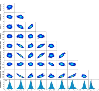
In Figure 6 we show the posterior PDFs for the nine fault source parameters obtained after 106iterations (a burn-in period of 2 × 10⁴iterations is removed), with the bottom row showing histograms of marginal distri-butions for each parameter and the remaining rows showing the joint distridistri-butions between pairs of para-meters. The maximum a posteriori probability solution and the 95% credible intervals are reported in Table 3.
The inversion reveals that coseismic surface displacements can be well explained by slip on a 19.5– 22.2-km-long and 7.6–11.7-km-wide fault, striking 113°–120° and shallowly dipping at 20°–29°. The slip direction is consistent with that of a thrust fault with a minor left-lateral component, with 0.4–0.6 m and 0.03–0.14 m of slip in the two directions, respectively. From the analysis of the marginal posterior probabilities (Figure 6), we can observe correlations between fault width, dip, and horizontal position. Conversely, we can well constrain the fault length, depth, strike direction, and the amount of slip in both the dip and strike directions. Assuming a shear modulus of 3.32 × 10¹⁰N/m2(Wen et al., 2016) and the marginal posterior prob-abilities for fault geometry and slip, the geodetic moment magnitudeMwis equal to 6.3 for the entire
prob-ability distribution, similar to the U.S. Geological Survey-National Earthquake Information Center and global centroid moment tensor solutions, and in agreement with previous studies of this earthquake (Ainscoe et al., 2017; He et al., 2016; Wen et al., 2016).
[image:13.612.35.578.122.204.2]In Table 4 we compare our inversion results with previous studies and show a consistent agreement in opti-mal source parameters. He et al. (2016) performed the source parameter optimization using a simplex algo-rithm but did not report how the associated uncertainties were estimated. The extremely narrow uncertainties they provide may represent an improper handling of errors in the data or an inappropriate approach in determining uncertainties. Wen et al. (2016) estimated optimal source parameters using a parti-cle swarm optimization and Ainscoe et al. (2017) using a downhill Powell’s algorithm. Both these last two stu-dies estimated model parameter uncertainties by running 100 and 250 inversions, respectively, of the InSAR data sets perturbed with simulated noise (e.g., Wright et al., 2003). Uncertainties estimated by Wen et al. (2016) seem still too optimistic while those by Ainscoe et al. (2017) are similar to our estimates obtained using the proposed Bayesian approach.
Table 3
Priors and Inversion Results for the 2015 Mw6.4 Pishan Earthquake
Rectangular dislocation with uniform slip (Okada, 1985)
Length (m) Width (m) Depth (m) Dip (°) Strike (°) Xcenter (m) Ycenter (m) Strike slipa(m) Dip slipb(m)
Lower 10,000 1,000 1,000 90 0 30,000 30,000 1.0 5.0
Upper 40,000 30,000 20,000 90 360 30,000 90,000 1.0 5.0
Optimal 20,736 9,448 11,932 25 116 1,399 55,842 0.09 0.51
2.5% 19,541 7,574 11,152 20 113 326 53,723 0.14 0.42
97.5% 22,179 11,675 12,413 29 120 2,139 57,089 0.03 0.63
6. Discussion
[image:14.612.176.572.80.444.2]Our Bayesian inversion framework is aimed at taking advantage of new opportunities offered by unprece-dented improvements in the availability and resolution, both temporal and spatial, of geodetic data. We show that with our approach, the inversion of net surface displacements from GNSS data, which in many cases are telemetered in real-time to geophysical monitoring facilities (e.g., https://www.unavco.org/data/
Table 4
Comparison of Results From Inversion of Interferometric Synthetic Aperture Radar Data for the 2015 Mw6.4 Pishan Earthquake
Rectangular dislocation with uniform slip (Okada, 1985)
Length (km) Width (km) Depth (km) Dip (°) Strike (°) Lon (deg) Lat (deg) Slipa(m)
This study 20.71.2/+1.4 9.41.9/+2.2 11.90.7/+0.5 255/+4 1163/+4 78.0161.1/+0.7 km 37.5032.1/+1.2 km 0.520.09/+0.11 He et al. (2016) 22.18 ± 0.05 8 N/A 10.98 ± 0.05 27.2 ± 0.2 113.8 ± 0.2 78.1390 ± 0.0004 37.7157 ± 0.00005 0.6 N/A Wen et al.
(2016)
22.1 ± 0.5 10.1 ± 1.0 8.8 ± 0.4 23.6 ± 1.5 114.0 ± 1.6 78.057 ± 0.4 km 37.571 ± 0.3 km 0.59 ± 0.06
Ainscoe et al. (2017)
21.5 ± 1.1 9.3 ± 2.1 11.0 ± 0.8 21 ± 2.5 112 ± 2.4 78.140 ± 1.7 km 37.777 ± 2.7 km 0.6 ± 0.2
Note. Data on previous studies as in Ainscoe et al. (2017).
[image:14.612.35.579.620.718.2]gps-gnss/real-time/real-time.html), can offer robust estimates of source parameters and uncertainties very rapidly (e.g., 3 min in the case of our synthetic GNSS data set). Similarly, we independently or jointly invert InSAR data to provide reliable estimates of deformation source parameters in 1.5–3.5 hr, depending on the size of the data sets. This becomes of unique value when using InSAR data from new satellite missions, such as Sentinel-1, which are acquired with much shorter revisit time (e.g., Sentinel-1, 6–12 days) and made avail-able within a few hours of acquisition.
For example, in March 2017 we applied our approach to an episode of volcanic unrest at Cerro Azul volcano (Galápagos Islands, Ecuador). Using the GBIS software, which implements our Bayesian inversion algorithm, we inverted InSAR data spanning a period of sudden and frequent seismicity beneath theflanks of the vol-cano. Within 5 hr from being alerted by Ecuador’s Instituto Geofisico-Escuela Politecnica National (Geophysical Institute-National Polytechnic School), we were able to access and process Sentinel-1 SAR data for the area of interest, which were acquired only a few hours earlier and which showed contemporary sub-sidence of the summit of the volcano and uplift of the lowerflank (e.g., Figure 7). The unwrapped interfero-grams were then inverted to gain information on the sources of surface displacements that were accompanying this episode of volcanic unrest, and inversion results were reported to Ecuador’s Instituto Geofisico-Escuela Politecnica National in less than 10 hr from receiving thefirst alert (http://www.igepn. edu.ec/servicios/noticias/1473-informe-especial-cerro-azul-no-2-2017). With this event, we demonstrated the potential of our approach for a quantitative interpretation of InSAR data in a rapid-response operational setting. In fact, our estimates of the credible interval of magma volumes involved in the volcanic unrest epi-sode were used by Ecuador’s Instituto Geofisico-Escuela Politecnica National to evaluate hazards associated with the event.
[image:15.612.221.532.90.305.2]When inverting InSAR data, a frequently applied alternative approach for the estimate of uncertainties in model parameters, also used in previous studies of the 2015 Pishan earthquake (see section 5; Ainscoe et al., 2017; Wen et al., 2016), implies the use of a nonlinear inversion technique capable offinding the weighted least-squares best-fit solution given the data plus simulated noise (e.g., Wright et al., 2003). This process is repeated several times (e.g., 102) using different simulations of the noise in the data, with the resulting distribution of solutions representing the posterior probability distribution of model parameters. While this approach and ours should provide similar results in cases were all priors are uniform, Hooper et al. (2010) showed that an MCMC approach, similar to the one presented here, is two orders of magnitude more efficient in terms of the number of forward models that need to be run, hence significantly faster.
Therefore, the Bayesian inversion approach may be preferable in rapid-response or operational settings (e.g., volcano observatories) and in all those cases where fast and robust estimates of source parameters may be needed. If prior probabilities on model parameters are also available, then the Bayesian approach is the only one capable of including these in the inversion. The rapidity of the inversion approach in estimating source parameters, especially in the case of a limited number of GNSS sites (e.g., GNSS data only in the validation example), can also be of use in the planning and design of geodetic monitoring networks. Through the use of synthetic data sets, the effect of a given measurement site can be quantified in terms of its contribu-tion to changes in source parameter uncertainties.
The proposed approach is aimed at the characterization of deformation source parameters through the inversion of static surface displacements spanning a given time interval. While this is of great value for early warning and in the rapid response to events of volcanic unrest and earthquakes, it is not optimized for the study of time-dependent dynamic processes. However, inversion results obtained through our approach are complementary and valuable in instructing other time-variable data assimilation algorithms (e.g., the ensemble Kalman Filter approach for volcano monitoring; Bato et al., 2017; Gregg & Pettijohn, 2016; Zhan & Gregg, 2017). Similarly, the Bayesian approach presented here can instruct or be extended to physical and dynamic models of geodetic and other geophysical measurements, as successfully demonstrated by Anderson and Segall (2013) in the study and forecasting of an episode of volcanic unrest.
Our Bayesian inversion framework aims at being applicable to different geophysical processes, in particular those related to tectonic and magmatic activity, and to both scientific research and natural hazard monitor-ing. To maintain theflexibility of the algorithm and its ability to efficiently invert different types of geodetic data for a multiplicity of deformation sources, we must rely on certain assumptions and reduce the level of complexity of certain steps. For example, a variety of one- and two-dimensional covariance functions could be applied to characterize errors in InSAR data (e.g., González & Fernández, 2011; Knospe & Jónsson, 2010), or different subsampling methods could be applied to subsample the data (see Section 3.2). While, at this stage, such complexities are not implemented in our approach and in the GBIS software, users can optionally adapt the algorithms to betterfit their aims and the desired level of complexity.
7. Conclusions
We have presented a Bayesian approach for the simultaneous inversion of independent geodetic data sets, in particular those from GNSS and InSAR, which takes into account errors in the data and prior information on model parameters. The inversion algorithm, which we implemented in the freely available MATLAB®-based GBIS software, is designed to rapidly estimate optimal model parameters and associated uncertainties through an efficient sampling of the posterior PDFs. Such sampling is performed using a MCMC method incorporating the Metropolis-Hastings algorithm and with an automatic step-size selection. We have applied the inversion method to synthetic GNSS and InSAR data sets and demonstrated its ability to retrieve the true input model parameters. We have also applied the same approach to InSAR data spanning a thrust earth-quake and retrieved source parameters for a rectangular fault with uniform slip. Our results are similar to those of previous studies that estimated uncertainties using the added simulated-noise method, but our methodology has been shown to be significantly faster in characterizing optimal model parameters and asso-ciated uncertainties, demonstrating its value in rapid-response and operational settings.
References
Ainscoe, E. A., Elliott, J. R., Copley, A., Craig, T. J., Li, T., Parsons, B. E., & Walker, R. T. (2017). Blind thrusting, surface folding, and the devel-opment of geological structure in theMw6.3 2015 Pishan (China) earthquake.Journal of Geophysical Research: Solid Earth,122, 9359–9382. https://doi.org/10.1002/2017JB014268
Amey, R. M., Hooper, A., & Walters, R. J. (2018). A Bayesian method for incorporating self-similarity into earthquake slip inversions.Journal of Geophysical Research: Solid Earth,123. https://doi.org/10.1029/2017JB015316
Anderson, K., & Poland, M. P. (2016). Bayesian estimation of magma supply, storage, and eruption rates using a multiphysical volcano model: Kilauea volcano, 2000–2012.Earth and Planetary Science Letters,447, 161–171. https://doi.org/10.1016/j.epsl.2016.04.029
Anderson, K., & Segall, P. (2013). Bayesian inversion of data from effusive volcanic eruptions using physics-based models: Application to Mount St. Helens 2004–2008.Journal of Geophysical Research: Solid Earth,118, 2017–2037. https://doi.org/10.1002/jgrb.50169 Auriac, A., Sigmundsson, F., Hooper, A., Spaans, K. H., Bjornsson, H., et al. (2014). InSAR observations and models of crustal deformation due to
a glacial surge in Iceland.Geophysical Journal International,198(3), 1329–1341. https://doi.org/10.1093/gji/ggu205
Bathke, H., Nikkhoo, M., Holohan, E. P., & Walter, T. R. (2015). Insights into the 3D architecture of an active caldera ring-fault at Tendürek volcano through modeling of geodetic data.Earth and Planetary Science Letters,422, 157–168. https://doi.org/10.1016/j.epsl.2015.03.041
Acknowledgments
Bato, M. G., Pinel, V., & Yan, Y. (2017). Assimilation of deformation data for eruption forecasting: Potentiality assessment based on synthetic cases.Frontiers in Earth Science,5(108), 1–12. https://doi.org/10.3389/feart.2017.00048
Battaglia, M., Cervelli, P. F., & Murray, J. R. (2013). DMODELS: A MATLAB software package for modeling crustal deformation near active faults and volcanic centers.Journal of Volcanology and Geothermal Research,254(July), 1–4. https://doi.org/10.1016/j.jvolgeores.2012.12.018 Biggs, J., & Pritchard, M. E. (2017). Global volcano monitoring: What does it mean when volcanoes deform?Elements,13(1), 17–22. https://doi.
org/10.2113/gselements
Cayol, V., & Cornet, F. H. (1997). 3D mixed boundary elements for elastostatic deformationfield analysis.International Journal of Rock Mechanics and Mining Science and Geomechanics Abstracts,34(2), 275–287. https://doi.org/10.1016/S0148-9062(96)00035-6
Cervelli, P., Murray, M. H., Segall, P., Aoki, Y., & Kato, T. (2001). Estimating source parameters from deformation data, with an application to the March 1997 earthquake swarm off the Izu Peninsula, Japan.Journal of Geophysical Research,106(B6), 11,217–11,237. https://doi.org/ 10.1029/2000JB900399
Currenti, G., Del Negro, C., & Nunnari, G. (2005). Inverse modelling of volcanomagneticfields using a genetic algorithm technique. Geophysical Journal International,163(1), 403–418. https://doi.org/10.1111/j.1365-246X.2005.02730.x
Decriem, J., Árnadóttir, T., Hooper, A., Geirsson, H., Sigmundsson, F., Keiding, M., et al. (2010). The 2008 May 29 earthquake doublet in SW Iceland.Geophysical Journal International,181(2), 1128–1146. https://doi.org/10.1111/j.1365-246X.2010.04565.x
Duputel, Z., Agram, P. S., Simons, M., Minson, S. E., & Beck, J. L. (2014). Accounting for prediction uncertainty when inferring subsurface fault slip.Geophysical Journal International,197(1), 464–482. https://doi.org/10.1093/gji/ggt517
Ebmeier, S. K., Andrews, B. J., Araya, M. C., Arnold, D. W. D., Biggs, J., Cooper, C., et al. (2018). Synthesis of global satellite observations of magmatic and volcanic deformation: Implications for volcano monitoring and the lateral extent of magmatic domains.Journal of Applied Volcanology,7(1), 2. https://doi.org/10.1186/s13617-018-0071-3
Elliott, J. R., Walters, R. J., & Wright, T. J. (2016). The role of space-based observation in understanding and responding to active tectonics and earthquakes.Nature Communications,7, 13844. https://doi.org/10.1038/ncomms13844
Fukuda, J., & Johnson, K. M. (2008). A fully Bayesian inversion for spatial distribution of fault slip with objective smoothing.Bulletin of the Seismological Society of America,98(3), 1128–1146. https://doi.org/10.1785/0120070194
Fukuda, J., & Johnson, K. M. (2010). Mixed linear-non-linear inversion of crustal deformation data: Bayesian inference of model, weighting and regularization parameters.Geophysical Journal International,181(3), 1441–1458. https://doi.org/10.1111/j.1365-246X.2010.04564.x González, P. J., & Fernández, J. (2011). Drought-driven transient aquifer compaction imaged using multitemporal satellite radar
interfero-metry.Geology,39(6), 551–554. https://doi.org/10.1130/G31900.1
González, P. J., Bagnardi, M., Hooper, A. J., Larsen, Y., Marinkovic, P., Samsonov, S. V., & Wright, T. J. (2015). The 2014–2015 eruption of Fogo volcano: Geodetic modeling of Sentinel-1 TOPS interferometry.Geophysical Research Letters,42, 9239–9246. https://doi.org/10.1002/ 2015GL066003
González, P. J., Walters, R. J.; Hatton, E. L., Spaans, K., & Hooper, A. J. (2016). LiCSAR: Tools for automated generation of Sentinel-1 frame interferograms. AGU FAll Meeting.
Gregg, P. M., & Pettijohn, J. C. (2016). A multi-data stream assimilation framework for the assessment of volcanic unrest.Journal of Volcanology and Geothermal Research,309, 63–77. https://doi.org/10.1016/j.jvolgeores.2015.11.008
Hanssen, R. F. (2001). Radar interferometry data interpretation and error analysis (p. 328). New York: Springer. https://doi.org/10.1007/0-306-47633-9
Hanssen, R. F., Weckwerth, T. M., Zebker, H. A., & Klees, R. (1999). High-resolution water vapor mapping from interferometric radar mea-surements.Science,283(5406), 1297–1299. https://doi.org/10.1126/science.283.5406.1297
Hastings, W. K. (1970). Monte Carlo sampling methods using Markov chains and their applications.Biometrika,57(1), 97–109. https://doi.org/ 10.1093/biomet/57.1.97
He, P., Wang, Q., Ding, K., Wang, M., Qiao, X., Li, J., et al. (2016). Source model of the 2015Mw6.4 Pishan earthquake constrained by inter-ferometric synthetic aperture radar and GPS: Insight into blind rupture in the western Kunlun Shan.Geophysical Research Letters,43, 1511–1519. https://doi.org/10.1002/2015GL067140
Herring, T. A., King, R. W., Floyd, M. A., & McClusky, S. C. (2015). GAMIT reference manual. Release 10.6. Mass. Inst. of Technol. Retrieved from http://geoweb. mit.edu/~simon/gtgk/GAMIT_Ref.pdf
Hooper, A., Ófeigsson, B., Sigmundsson, F., Lund, B., Einarsson, P., Geirsson, H., & Sturkell, E. (2011). Increased capture of magma in the crust promoted by ice-cap retreat in Iceland.Nature Geoscience,4(11), 783–786. https://doi.org/10.1038/ngeo1269
Hooper, A., Pietrzak, J., Simons, W., Cui, H., Riva, R., Naeije, M., et al. (2013). Importance of horizontal seafloor motion on tsunami height for the 2011Mw= 9.0 Tohoku-Oki earthquake.Earth and Planetary Science Letters,361, 469–479. https://doi.org/10.1016/j. epsl.2012.11.013
Hooper, A., Wright, T. J., & Systems, S. (2010). Comparison of Monte Carlo methods for model probability distribution determination in SAR interferometry.Earth,2009(March), 2–6.
Jeffreys, H. (1939). Theory of probability, Clarendon Press, Oxford. Reprinted in 1961 by Oxford University Press.
Jolivet, R., Simons, M., Agram, P. S., Duputel, Z., & Shen, Z.-K. (2015). Aseismic slip and seismogenic coupling along the central San Andreas fault.Geophysical Research Letters,42, 297–306. https://doi.org/10.1002/2014GL062222
Jonsson, S. (2002). Fault slip distribution of the 1999Mw7.1 Hector Mine, California, earthquake, estimated from satellite radar and GPS measurements.Bulletin of the Seismological Society of America,92, 1377–1389. https://doi.org/10.1785/0120000922
Juncu, D., Árnadóttir, T., Hooper, A., & Gunnarsson, G. (2017). Anthropogenic and natural ground deformation in the Hengill geothermal area, Iceland.Journal of Geophysical Research: Solid Earth,122, 692–709. https://doi.org/10.1002/2016JB013626
Knospe, S. H. G., & Jónsson, S. (2010). Covariance estimation for dInSAR surface deformation measurements in the presence of anisotropic atmospheric noise.IEEE Transactions on Geoscience and Remote Sensing,48(4 PART 2), 2057–2065. https://doi.org/10.1109/TGRS.2009.2033937 Lisowski, M. (2007). Analytical volcano deformation source models. InVolcano deformation, (pp. 279–304). Berlin: Springer Praxis Books.
Retrieved from papers://8461d6ef-418445b2-aa3d-395291ea6525/Paper/p15
Lohman, R. B., & Simons, M. (2005). Some thoughts on the use of InSAR data to constrain models of surface deformation: Noise structure and data downsampling.Geochemistry, Geophysics, Geosystems,6, Q01007. https://doi.org/10.1029/2004GC000841
McTigue, D. F. (1987). Elastic stress and deformation near afinite spherical magma body: Resolution of the point source paradox.Journal of Geophysical Research,92(B12), 12931. https://doi.org/10.1029/JB092iB12p12931
Metropolis, N., Rosenbluth, A. W., Rosenbluth, M. N., Teller, A. H., & Teller, E. (1953). Equation of state calculations by fast computing machines. The Journal of Chemical Physics,21(6), 1087–1092. https://doi.org/10.1063/1.1699114
Mosegaard, K., & Tarantola, A. (1995). Monte Carlo sampling of solutions to inverse problems.Journal of Geophysical Research,100(B7), 12,431–12,447. https://doi.org/10.1029/94JB03097
Okada, Y. (1985). Surface deformation due to shear and tensile faults in a half-space Okada, Y Bull Seismol Soc AmV75, N4, Aug 1985, P1135–
1154.International Journal of Rock Mechanics and Mining Science and Geomechanics Abstracts,75, 1135–1154. https://doi.org/10.1016/ 0148-9062(86)90674-1
Pinel, V., Poland, M. P., & Hooper, A. (2014). Volcanology: Lessons learned from synthetic aperture radar imagery.Journal of Volcanology and Geothermal Research,289, 81–113. https://doi.org/10.1016/j.jvolgeores.2014.10.010
Pritchard, M. E., Simons, M., Rosen, P. A., Hensley, S., & Webb, F. H. (2002). Co-seismic slip from the 1995 July 30Mw= 8.1 Antofagasta, Chile, earthquake as constrained by InSAR and GPS observations.Geophysical Journal International,150(2), 362–376. https://doi.org/10.1046/ j.1365-246X.2002.01661.x
Roberts, G. O., Gelman, A., & Gilks, W. R. (1997). Weak convergence and optimal scaling of random walk Metropolis algorithms.Annals of Applied Probability,7(1), 110–120. https://doi.org/10.1214/aoap/1034625254
Roberts, G. O., & Rosenthal, J. S. (2001). Optimal scaling for various Metropolis-Hastings algorithms.Statistical Science,16(4), 351–367. https:// doi.org/10.1214/ss/1015346320
Sahlin, K. (2011). Estimating convergence of Markov chain Monte Carlo simulations.Annals of Biomedical Engineering,32(9), 1300–1313. Retrieved from http://www.ncbi.nlm. nih.gov/pubmed/15493516
Sambridge, M., & Mosegaard, K. (2002). Monte Carlo methods in geophysical inverse problems.Reviews of Geophysics,40(3), 1009. https://doi. org/10.1029/2000RG000089
Samsonov, S. V., González, P. J., Tiampo, K. F., & D’Oreye, N. (2014). Modeling of fast ground subsidence observed in southern Saskatchewan (Canada) during 2008–2011.Natural Hazards and Earth System Sciences,14(2), 247–257. https://doi.org/10.5194/nhess-14-247-2014 Segall, P. (2010).Earthquake and volcano deformation. Princeton, NJ: Princeton University Press. https://doi.org/10.1002/0471743984.
vse7429
Shirzaei, M., & Walter, T. R. (2009). Randomly iterated search and statistical competency as powerful inversion tools for deformation source modeling: Application to volcano interferometric synthetic aperture radar data.Journal of Geophysical Research,114, B10401. https://doi. org/10.1029/2008JB006071
Sigmundsson, F., Hooper, A., Hreinsdóttir, S., Vogfjörd, K. S., Ófeigsson, B. G., Heimisson, E. R., et al. (2014). Segmented lateral dyke growth in a rifting event at Bárðarbunga volcanic system, Iceland.Nature,517(7533), 191–195. https://doi.org/10.1038/nature14111
Simons, M. (2002). Coseismic deformation from the 1999Mw7.1 Hector Mine, California, earthquake as inferred from InSAR and GPS observations.Bulletin of the Seismological Society of America,92(4), 1390–1402. https://doi.org/10.1785/0120000933
Sudhaus, H., & Jónsson, S. (2009). Improved source modelling through combined use of InSAR and GPS under consideration of correlated data errors: Application to the June 2000 Kleifarvatn earthquake, Iceland.Geophysical Journal International,176(2), 389–404. https://doi. org/10.1111/j.1365-246X.2008.03989.x
Ulrych, T. J., Sacchi, M. D., & Woodbury, A. (2001). A Bayes tour of inversion: A tutorial.Geophysics,66(1), 55–69. https://doi.org/10.1190/ 1.1444923
Wackernagel, H. (1995). Variogram and covariance function. InMultivariate Geostatistics(pp. 35–40). Berlin: Springer. https://doi.org/10.1007/ 978-3-662-03098-1_5
Wang, C., Ding, X., Li, Q., & Jiang, M. (2014). Equation-based InSAR data quadtree downsampling for earthquake slip distribution inversion. IEEE Geoscience and Remote Sensing Letters,11(12), 2060–2064. https://doi.org/10.1109/LGRS.2014.2318775
Wen, Y., Xu, C., Liu, Y., & Jiang, G. (2016). Deformation and source parameters of the 2015Mw6.5 earthquake in Pishan, western China, from sentinel-1A and ALOS-2 data.Remote Sensing,8(2), 1–14. https://doi.org/10.3390/rs8020134
Wright, T. J., Lu, Z., & Wicks, C. (2003). Source model for theMw6.7, 23 October 2002, Nenana Mountain earthquake (Alaska) from InSAR. Geophysical Research Letters,30(18), 1974. https://doi.org/10.1029/2003GL018014