This is a repository copy of
Atoms in complex twisted light
.
White Rose Research Online URL for this paper:
http://eprints.whiterose.ac.uk/141716/
Version: Published Version
Article:
Babiker, Mohamed Elhag orcid.org/0000-0003-0659-5247, Andrews, D L and Lembessis,
Vassilis (2018) Atoms in complex twisted light. Journal of Optics. 013001-013068. ISSN
2040-8986
https://doi.org/10.1088/2040-8986/aaed14
[email protected] https://eprints.whiterose.ac.uk/
Reuse
This article is distributed under the terms of the Creative Commons Attribution (CC BY) licence. This licence allows you to distribute, remix, tweak, and build upon the work, even commercially, as long as you credit the authors for the original work. More information and the full terms of the licence here:
https://creativecommons.org/licenses/
Takedown
If you consider content in White Rose Research Online to be in breach of UK law, please notify us by
Journal of Optics
TOPICAL REVIEW • OPEN ACCESS
Atoms in complex twisted light
To cite this article: Mohamed Babiker et al 2019 J. Opt. 21 013001
View the article online for updates and enhancements.
Recent citations
Quadrupole Interaction of Non-diffracting Beams with Two-Level Atoms
Saud Al-Awfi and Smail Bougouffa
Topical Review
Atoms in complex twisted light
Mohamed Babiker
1, David L Andrews
2and Vassilis E Lembessis
3 1Department of Physics, University of York, Heslington, York YO10 5DD, United Kingdom 2School of Chemistry, University of East Anglia, Norwich NR4 7TJ, United Kingdom3Quantum Technology Group, Department of Physics and Astronomy, College of Science, King Saud
University, Riyadh 11451, Saudi Arabia
E-mail:[email protected]
Received 21 March 2018, revised 20 August 2018 Accepted for publication 31 October 2018 Published 18 December 2018
Abstract
The physics of optical vortices, also known as twisted light, is now a well-established and a growing branch of optical physics with a number of important applications and significant inter-disciplinary connections. Optical vortexfields of widely varying forms and degrees of complexity can be realised in the laboratory by a host of different means. The interference between such beams with designated orbital angular momenta and optical spins(the latter is associated with wave polarisations)can be structured to conform to various geometrical arrangements. The focus of this review is on how such tailored forms of light can exert a controllable influence on atoms with which they interact. The main physical effects involve atoms in motion due to application of optical forces. The now mature area of atom optics has had notable successes both of fundamental nature and in applications such as atom lasers, atom guides and Bose–Einstein condensates. The concepts in atom optics encompass not only atomic
beams interacting with light, but atomic motion in general as influenced by optical and other fields. Our primary concern in this review is on atoms in structured light where, in particular, the twisted nature of the light is made highly complex with additional features due to wave polarisation. These features bring to the fore a variety of physical phenomena not realisable in the context of atomic motion in more conventional forms of laser light. Atoms near resonance with such structured lightfields become subject to electromagneticfields with complex polarisation and phase distributions, as well as intricately structured intensity gradients and radiative forces. From the combined effect of optical spin and orbital angular momenta, atoms may also experience forces and torques involving an interplay between the internal and centre of mass degrees of freedom. Such interactions lead to new forms of processes including scattering, trapping and rotation and, as a result, they exhibit characteristic new features at the micro-scale and below. A number of distinctive properties involving angular momentum exchange between the light and the atoms are highlighted, and prospective applications are discussed. Comparison is made between the theoretical predictions in this area and the corresponding experiments that have been reported to date.
Keywords: twisted light, atoms, optical angular momentum, structured light, optical vortex, optical manipulation, quantum electrodynamics
(Somefigures may appear in colour only in the online journal)
J. Opt.21(2019)013001(67pp) https://doi.org/10.1088/2040-8986/aaed14
List of symbols and abbreviations
A
⊥ transverse electromagnetic vector potentialB magnetic vectorfield; also represents artificial vector magneticfield
C∣ ∣l p Laguerre–Gaussian mode normalisation constant
d electric dipole moment
E⊥ transverse electric vectorfield
electric field vector Erec atom recoil energy
F
á ñ average force H total Hamiltonian Hint interaction Hamiltonian I light intensity
IS saturation intensity
J current density
Jl(x) Bessel function of the first kind of orderl
k wavevector
Lagrangian density L total Lagrangian
L orbital angular momentum density operator l winding number (azimuthal index) in a
twisted beam
lin lin^ linearly polarised light beams, with orthogonal polarisations
Lp l
∣ ∣ associated Laguerre polynomial fi
matrix element of interaction HamiltonianHint between quantum statesiand f
M mass of the two-particle atom
magnetic dipole moment
pα=1,2 momentum canonically conjugate toqα=1,2
p radial nodal index in a twisted beam
electric polarisation vector T
truncated electric polarisation vector (up to quarupole term)
qα=1,2 particle position vector in the two-particle
(hydrogenic)atom
Qij (ij)th component of the electric quadrupole
moment tensor
R atomic centre of mass position vector variable
S˜ optical spin angular momentum density
S optical chirality flux
S optical linear momentum density vector s0 saturation parameter
torque on atomic centre of mass
U
á ñ dipole potential
up∣ ∣l LG amplitude distribution function
R
V= ˙ velocity vector of the atomic centre of mass
V(R) artificial gauge scalar field of atom in an
opticalfield
vD the Doppler velocity vrec recoil velocity vg group velocity
w(z) beam waist at positionzin the beam zR Rayleigh range
αF damping coefficient in Sisyphus cooling αf azimuthal damping coefficient in Sisyphus
cooling
a˜ atomic polarisability
Δ detuning of light frequency from atomic transition frequency
Δ0 static detuning δ doppler shift
r r
ij
d^( - ¢) transverse Dirac delta function òf two-level atom adiabaticity parameter ò adiabaticity parameter
¢ non-adiabaticity parameter in Sisyphus effect Φ artificial magneticflux
j optical chirality density
Γ upper state de-excitation rate in a two-level atom
κ scalarfield helicity
λ wavelength
Λ generating function in a Power–Zienau–
Wool-ley(PZW)gauge transformation
k10
L elastic modulus of LG donut dipole trap
P^ momentum canonically conjugate toA⊥ 0
p canonical momentum density of evanescent light s
p spin momentum density of evanescent light s^ wavepacket transverse spread
s˜ evanescent wave helicity
Θklp Laguerre–Gaussian phase function
σ± left and right handed circular polrisation of light
Ω rabi frequency
Ω0 rabi frequency associated with beam ampl-itudeEk00
Ψ atomic state function on diffraction in atom vortices
AVB atom vortex beam HOT helical optical tube LG Laguerre–Gaussian OAM orbital angular momentum SOV surface optical vortex
SPOV surface plasmon optical vortices
1. Introduction
The term‘twisted light’refers to various states of light which are endowed with the property of orbital angular momentum
(OAM). These encompass a wide range, including twisted light in freely propagating beams such as Laguerre–Gaussian
(LG) and Bessel beams[1] and other forms of twisted light inside opticalfibres[2]and onfibres supporting twisted light
[3], as well as wave guide arrays [4]. Twisted light modes have also featured in nonlinear waveguides [5] and as so-called surface optical vortices (SOVs)[6]. The reference to the twisted nature stems from the observation that the OAM property of the light makes the normal to its wave-fronts twist in a helical fashion with a degree of twisting depending on the OAM content. Freely propagating twisted beams are proto-typical twisted light and were thefirst to be explored; they are also referred to as optical vortex beams. It has been realised
[7]that associated with the wave-front of such a state of light
is a topological structure due to a singularity in phase. In cylindrical polar coordinates (ρ, f, z) the phase of a pure vortex state takes the formexp(ilf)wherelis the topological charge, also called the‘winding number’and the‘azimuthal quantum number’. The value of∣ ∣l also quantifies, in terms of the reduced Planck constant ÿthe OAM conveyed per pho-ton. Nye and Berry were thefirst to describe the topological features of the wave-front as a screw dislocation in a manner similar to that encountered in crystal defects[8].
This review is concerned with the principles, recent developments and applications in the context where atoms interact with twisted light. Here we begin with the back-ground theory of the interaction of atoms with electro-magnetic fields in general, emphasising the division of the atom dynamics into gross motion associated with the centre of mass (which is dominated by the nuclear mass) and the internal motion involving the bound electrons, and the dis-tinction between optical spin and optical OAM densities. This is followed by brief descriptions of conventional laser cooling and trapping of atoms, including Doppler and Sisyphus mechanisms. The essential formalism for twisted lightfields is given next with emphasis on LG light as the most widely discussed form of twisted light. The inclusion of optical wave polarisation (photon spin) as one of the main sources of
complexity of the twisted light is discussed with special emphasis on polarisation gradients arising in co- and counter-propagating twisted light beams with circular polarisations. This background sets the scene for the main aim of this review, namely the description arising when complex twisted light interacts with atoms.
One of thefirst issues to be addressed in the context of twisted light interaction with atoms is the possibility of exchange of OAM. Could the well known selection rules in the case of emission and absorption of ordinary (Gaussian)
polarised light with atoms be modified with the involvement of the new ingredient in the form of OAM carried by twisted light? The theory of this process is based on the analysis of the transition matrix element for dipolar and quadrupolar active transitions and on the division between the centre of mass and the internal (electronic-type) motion of the atom.
We highlight experiments carried out to date on this issue. The interaction also gives rise to modified optical forces that act on the centre of mass of the atom with additional char-acteristic features associated with the OAM content of the twisted light, including azimuthal Doppler shifts along with azimuthal forces and torques about the beam propagation direction and an azimuthal Sisyphus effect. Multiple beams are shown to lead to‘twisted molasses’and other novel forms of optical trapping, including the formation of‘Ferris wheels’
and ‘HOTs’ which arise when co-propagating beams with opposite and identical winding numbers are formed.
Totally internally reflected twisted light can generate
SOVs as evanescent waves carrying OAM and in the pre-sence of a metallic film deposited on the surface, the
eva-nescent modes acquire a plasmonic character. Such evanescent fields interact with atoms in the vicinity of the surface and the atoms may become trapped in the surface region.
LG twisted light beams have anomalous additional phase effects due to being focused beams with a well-defined waist plane at focus. The additional phase terms in the form of a Gouy phase and a curvature phase term are normally ignored but become significant for atoms localised the vicinity of the focus plane, particularly for LG light with large values of winding number land/or radial number p. Under these cir-cumstances the atoms experience enhanced anomalous phase effects in the form of modified gradient forces which can
diminish the axial force component acting on the atom, or even reverse its direction.
Besides LG and Bessel beams where the dominant phase involves integer winding number l, light beams with frac-tional OAM have been considered. In particular, Götteet al
[9]reported the generation of light carrying fractional OAM
by limiting the number of Gouy phases in a superposition of LG light beams.
A well defined beam of atoms, like an optical beam, is essentially a de Broglie wave with a wavelength that depends on the atomic axial velocity. Diffraction through light masks, in techniques somewhat akin to, but rather different from, those used for the generation of twisted light, are expected to lead to the generation of twisted beams of atoms, so-called
‘atom vortex beams’. Finally, we describe how the gross
motion of atoms in twisted light gives rise to artificial gauge fields for atoms in donut modes and in Ferris wheel patterns.
In the conclusions section, we briefly identify a number
of other treatments of atoms in twisted light that are beyond our scope in this review, including the trapping of ions in donut beams, the effects on cyclotron motion of ions in twisted light, spin–orbit coupling effects in this context and nonlinear effects.
2. Coupling light to atoms
The essential background physics describing the interaction of twisted light with atoms stems from conventional non-relativistic quantum electrodynamics [10] and considerable
subject to light typically exhibits two kinds of dynamics, namely the dynamics involving the gross motion of the atom as a whole, in terms of its centre of mass, and processes involving the internal dynamics in the form of transitions between quantum(electronic)states due to the emission and absorption of light quanta. These features play central roles in the context of twisted light interacting with atoms and it is helpful to tailor the formalism in a manner that highlights the roles of the internal and gross motions. It is common practice to explore interactions of atoms and molecules in terms of multipole moments, both electric and magnetic, coupled to the electromagnetic fields [13, 16]. The treatment becomes
particularly simple, but perfectly adequate and transparent, when the atom comprises an outer electron and a nucleus surrounded by a closed-shell electron core. The corresp-onding particles have nett charges e1=-∣ ∣e (electron) and
e2=+∣ ∣e (nucleus and core)and massesm1=me(electronic mass),m2=mc(nucleus and core). Any inner transitions of the core need not concern us. We must bear in mind that m2?m1, but it is important not to impose this condition
from the outset, in order to fully take account of the centre of mass motion and its coupling to both the relative motions of the outer electron and core and the light fields. The two-particle atom coupled to the electromagnetic field has the following non-relativistic classical Lagrangian in the trans-verse(radiation)gauge[16]
L mq m q e e d
q q r
1 2
1
2 4 , 1
1 12 2 22 1 2 0 1 2
ò
p = + -- + ˙ ˙ ∣ ( ) where c
J A 1 A A
2 0 , 2
2 2
2
= · ^+ [ ˙^ - (´ ^) ] ( ) withqaandq˙a,a=1, 2, the particle position variables and corresponding velocity vectors. In the radiation gauge
A 0
^=
( · ) the Coulomb effects reside in the static inter-particle interaction and we only have A⊥ as the canonical field variable. Besides the Coulomb interaction, the coupling
between thefield and the particles occurs via the total current
density
e e
J r( )= 1 1q˙ (d r-q1)+ 2q˙ (2d r-q2). ( )3 The dynamical variables in this canonical procedure areq1,q2
andA r^( ), and the corresponding canonical momenta arep1,
p2 and P^( ). These canonical momenta emerge from ther
Lagrangian as follows
L
m e
p
q q A q ; a 1, 2, 4
= 
¶ = - =
a
a a a a a
^
˙ ˙ ( ) ( )
A A
E , 5
0 0
P = 
¶ = =
-^
^
^ ^
˙ ˙ ( )
and we obtain the total Hamiltonian in the form
H e m e m e e c d
p A q p A q
q q E B r
2 2
4
1
2 . 6
1 1 1 2
1
2 2 2 2
2
1 2
0 1 2
0 2 2
2
ò
p = + + + + - + + ^ ^ ^ ∣ ( )∣ ∣ ( )∣ ∣ ∣ ( ) ( )
The transition to the corresponding quantum theory fol-lows once we identify the canonical momentum and coordi-nate variables as operators obeying commutation rules
p q i
A r t r t i r r
, ,
, , , , 7
i j ij
i j ij
d d d =
-P ¢ = - ¢
a b ab
^ ^ ^
[ ]
[ ( ) ( )] ( ) ( )
wheredij^( )r is the transverse delta function[10]. The above
framework constitutes the non-relativistic QED theory for the two-particle atom interacting with light. However, so far the theory deals with two individual charged particles interacting with each other and with electromagnetic fields. We need to devise means of identifying features of the dynamics which recognise its division into types belonging to internal and gross motions. The most useful form occurs when we seek to express the Hamiltonian in equation(6)in a multipolar form. The complete theory can be generalised to a many-body system involving atoms and molecules with well defined
centres. Such a theory is now known as the Power–Zienau–
Woolley(PZW)theory, with numerous groups contributing to
its development and analysis(see[11–29]). The key point is
the observation that it is possible to take account of all mul-tipoles, both electric and magnetic in closed forms and for-mally include inter- as well as intra-centre interactions [12].
As we emphasise above, the version of the theory in which we deal with a one-centre atom is both instructive and rela-tively simple. Our ultimate aim in the context of this model is to arrive at a Hamiltonian which is valid to all multipolar orders, but ultimately we shall need to highlight applications involving the leading electric dipole and quadrupole interac-tions, as these are the multipolar orders currently accessible to experimental work, including recent experiments on OAM exchange between atoms and twisted light.
We begin by introducing the total electric polarisation vectorfield( )r for the two-particle system in the form
e d
r q R r R q R ,
8
1,2 0
1
=
å
-ò
ld - -l-a
a a a
=
( ) ( ) [ ( )]
( ) in whichλis an integration parameter andRis the centre of mass position vector
m m
M M m m
R= 1 1q 2q2; 1 2. 9
+
= + ( )
The above expression of the electric polarisationfield of the
two-particle system is a closed expression representing con-tributions from all electric multipoles excluding any net monopole(which can be included separately, e.g. in the case
of an atomic ion). The multipoles manifest themselves on
expanding the delta function appearing in( )r in powers of
(qα−R), α=1, 2. These two vectors are related to the internal coordinate of the two-particle system denoted byq
q=q1-q2, ( )10
and it is easy to show thatq1−R=m2q/Mandq2-R=
m1q M
- . Making use of these relations, the polarisation vector field can be written entirely in terms of the internal
coordinatesqand thefield position variabler. By expanding
the delta functions in (8) in powers of q followed by inte-gration over λ yields the ith Cartesian component of the expanded polarisation field vector. Up to the quadrupole moment, we have (using the Einstein convention that a repeated index is summed over a set of mutually orthogonal coordinates)
d Q
r 1 r R
2 , 11
i i ij j
»⎡ + d
-⎣⎢
⎤ ⎦⎥
( ) ( ) ( )
where d=∣ ∣eq is the electric dipole moment and Qij=
e q qi j
∣ ∣ is a(ij)th component of the electric quadrupole moment
tensor. For electric dipole-active transitions, only the first
term is applicable, while the second (quadrupole) term
dominates in case of dipole forbidden transitions.
In practice, one seldom goes beyond this truncated form of the electric polarisation as given in equation (11) and, unless otherwise stated, it is this form that we shall need when it comes to applications involving the coupling of the twisted light to atomic systems. Ultimately, it will prove convenient to use the notationT( )r to refer to the truncated polarisation
vectorfield, which we will subsequently define as follows
r D r R, 12
T
( )» d( - ) ( )
where D is a quadrupole-corrected dipole moment operator with components given by
d Q
D 1
2 . 13
i= i+ ijj ( )
2.1. Canonical transformation
The coupling of the light to all the atomic multipoles is achievable via a PZW canonical transformation or, equiva-lently, a gauge transformation involving a characteristic generating functionS in the form[13,16]
eiS e i r A rdr. 14
ò
L = = - ( )· ( )^ ( )
This unitary transformation gives rise to a new Hamiltonian Hnewwhich has the same form as the old HamiltonianH, and to mark the distinction we now represent all transformed canonical variables with a prime. We have
H e m e m e e d
p A q p A q
q q B r 2 2 4 1
2 . 15
new 1 1 1
2
1
2 2 2 2
2
1 2
0 1 2 0
2
0
2
ò
p m P = ¢ + + ¢ + + - + ¢ + ^ ^ ^ ⎛ ⎝ ⎜ ⎞ ⎠ ⎟ [ ( )] [ ( )] ∣ ∣ ( )
After transformation, the new momentap¢aandP¢^are given by
e e i S
p¢ = iSp iS =p + p , , 16
a - a a [ a ] ( )
e iS eiS i ,S . 17
P¢ =^ - P^ =P^+ [P^ ] ( )
The evaluations of equations (16) and (17) both involve a
commutator series, but it is easy to verify that both series terminate at thefirst commutator in each case due to the form
ofSin equation(14). Wefind
S
p¢ =a pa+a , ( )18
r r r, 19
P¢^( )=P^( )- ^( ) ( )
where a in equation (18) denotes differentiation with
respect to the canonical coordinate qα. The vector field ^ appearing in equation (19) stands for the transverse vector
field part of the electric polarisation vector field given in equation(8), having made use of the commutation relations in equation(7).
The formal multipolar Hamiltonian follows from equation (15)by direct use of equations (18) and (19). The next steps involve the division of the motion into the internal motion (which is characterised by the appearance of the relative coordinate q), and the gross motion involving the centre of mass coordinateR.
2.2. Decoupling of motions
Although we can continue the treatment without further recall of a multipolar expansion, it is instructive to focus again on the approximation in which the electric polarisation vector
field takes its truncated form in equation (11) with leading
contributions including only the electric dipole and the elec-tric quadrupole terms We obtain foraS after some algebra
S e A q 1D B R
2 . 20
a = - a + ´
a
^( ) ( ) ( )
Hence we can write for the transformed momenta, equations(18)and(19)
e
p p A q 1D B R
2 , 21
¢ =a a- a ^( )a + ´ ( ) ( )
r r r. 22
P¢^( )=P^( )- ^( ) ( )
Note that the last term in equation(21)does not depend onα. Finally, substituting from equations (21) and (22) in equation(15), we obtain the transformed Hamiltonian in the following form
H
m
e
d
p D B R
r r B r
r
2 4 q
1
2 . 23
new 1,2 1 2 2 2 0 2 0 2 0
ò
å
p m P = + ´ -+ - + a a a = ^ ^ ⎧ ⎨ ⎩ ⎫ ⎬ ⎭ ( ) ∣ ( ) ( )∣ ( ) ( )To arrive at a theory with explicit division of the motion into internal and gross motions, we have to define the centre of mass momentumP conjugate to the centre of mass position vectorR, as defined in equation(9)
P=p1+p2 ( )24
and the internal momentump conjugate to the internal vari-ableqby
m m
M
p= 2 1p - 1 2p ; q=q1-q2. ( )25 We can then expressp1andp2in terms ofPandpas follows
m M
p = P+ -1 1p; a=1, 2. 26
a a ( )a+ ( )
Equation(26) enables the explicit change from the
par-ticle canonical variablesqaandpαto internal variables(q,p) and gross motion variables (R, P). That the new pairs are independent canonical variables can easily be checked. We have [P , Ri j]= -idij; p , q[ i j]= -idij and [P , qi j]= =0
p , Ri j
[ ] which follow by direct use of the commutator
i
p , qai bj = -d dab ij.
[ ] The above commutator relationships ensure that the new variables conform with the requirements for independent sets representing two independent motions in the absence of coupling. Substituting from equation(26) in equation(23), we get
27 H m m e d
p D B R
r r B r
r 1 2 4 q 1 2 . new M P 1,2 1 1 2 2 2 0 2 0 2 0
ò
å
p m P = + - + ´ - + - + a a a a = + ^ ^ ⎛ ⎝ ⎜ ⎜ ⎜ ⎞ ⎠ ⎟ ⎟ ⎟ ⎡ ⎣ ⎢ ⎤ ⎦ ⎥ ( ) ( ) ( ) ∣ ( ) ( )∣ ( )The Hamiltonian (27)simplifies considerably on expanding the square and wefind
H M e B d M d P p r r
r D R
P D B R D B R P
D B R
r r B R
2 2 4 q
1 2
1 .
1
2 . .
8
1
2 ,
28 new
2 2 2
0 2 0 2 0 0 2 0 2
ò
ò
m p m m P = +-+ P + +
+ ´ + ´ + ´ + + ^ ^ ^ ⎛ ⎝ ⎜ ⎞ ⎠ ⎟ ⎛ ⎝ ⎜ ⎞ ⎠ ⎟ ( ) ( ) ( ) ( ( ) ( ) ) [ ( )] ( ) · ( ) ( ) where μ is the reduced massm=(m m1 2) M and coupling
terms are given in the truncated approximation. The ultimate term involves the magnetic moment coupling to the magneticfield also in the truncated approximation. This term arises from the product betweenpandD×B. In the dipole approximation whereD=d, the leading contribution to the
magnetic dipole moment is
m d p
1
2 e . 29
= ´ ( )
Equation(28)is the non-relativistic Hamiltonian for the
electrically neutral two-particle atom in interaction with light. It is seen that the internal electronic-type motion is essentially separated from the gross motion, but these two subsystems of the atom are coupled by mutual interactions between charges and with the lightfields. Amongst the various terms there are three that essentially represent unperturbed components of the system; these are the(zero-order)Hamiltonians representing the gross (centre of mass) motion, the internal ( electronic-type) motion and the light fields—which appear as thefirst three terms of equation(28). Other terms represent couplings between the three subsystems; the fourth term represents the coupling of the atomic dipole as well as the quadrupole moments to the transverse part of the displacementfieldP^ (evaluated at the centre of mass coordinate R); the fifth
constitutes the leading interaction involving the centre of
mass with the truncated multipole moment and the magnetic
field; the sixth is the diamagneticfield-type energy and the seventh term is an integral of the square of the polarisation
field. The latter is a self energy contributing to the Lamb shift and may be absorbed in any renormalised energies pertaining to the internal motion. Finally, the last term is the leading interaction between the magnetic dipole of the atom and the magneticfield of the light, evaluated at the centre of massR.
2.3. Mechanical momentum and pressure force
A prominent feature of the Hamiltonian in equation (28),
when taken in the truncated multipole approximation is the appearance of the term D×B. In the electric dipole approximation, this can be written as eAR where
AR=q×B. ClearlyARplays the role of an electrodynamic vector potential. The significance of this can readily be seen by considering the particle canonical momenta. From equation(21), we can write
e
p A q p 1D B R
2 . 30
¢ +a a ^ a = a+ ´
( ( )) ( ) ( )
The left hand side is equal toma aq˙ , so we can write
m q p 1D B R
2 . 31
= + ´
a a˙ a ( ) ( )
Summation overα=1, 2 in all terms we get
m q p D B R. 32
1,2 1,2
å
=å
+ ´a= a a a= a
˙ ( ) ( )
Using equation (9), the left hand side of equation (32) is exactlyMR˙ while thefirst term on the right hand side is just P. We therefore have
MR˙ =P+D´B R( ). ( )33 The relationship in(33)is between the canonical momentum
Pand the mechanical momentumMR˙ of the centre of mass in the truncated multipole approximation. The result also fol-lows as a Heisenberg operator equation based on the Hamiltonian in equation (28). We have,
i H
M
R new,R P D B R . 34
= = + ´
˙ [ ] ( ( )) ( )
The radiation pressure force acting on the centre of mass in the dipole approximation follows from equation(33)by total
time differentiation d dt M d dt d dt
F= ( ˙ )R = P + (D´B). ( )35 The force also follows from equation (34) as a Heisenberg operator equation in the form
M i H
d dt
R P D B
D E R D B
¨ , , 36 new = + ´ = - + ´ [ ( )] ( · ( )) ( ) ( )
where refers to differentiation with respect to the compo-nents ofR. We have explicitly evaluated thefirst commutator
H ,P D E
i new
[ ]=( · )but left the second commutator as a
time derivative. The last term is referred to as the Röntgen force, generalised here to include the quadrupole contribution. The so-called Röntgen effect arises when an electrically neutral system possessing a dipole moment is in motion in a magnetic field [19]. Here, we have shown that the
corresp-onding interaction arises from a treatment incorporating the motion of the atomic centre of mass as a dynamical variable. Other effects that have been predicted to arise from the motion of neutral quantum systems include the rotational motion of a BEC with a form of distribution effectively associated with either a magnetic monopole distribution or an electric charge distribution [20]. We have therefore
estab-lished that both dynamical attributes, namely the momentum and the corresponding pressure force, receive contributions directly attributable to the Röntgen interaction. The complete Hamiltonian in the truncated pole approximation is essential for studying processes involving the coupling of the atomic system to electromagneticfields.
The multipolar theory of atom-field interactions,
begin-ning with the seminal work by Power and Zienau [21]was
subsequently developed and applied by several contributors. The reader is referred to the following sources for further information[22–29].
2.4. Quantum amplitudes and motion
Before proceeding further, it is helpful to recognise two quite distinct forms of mechanical response that arise in describing the evolution of a given atom + radiation state. As fully discussed elsewhere [30, 31], gradient forces are generally
produced in response to interactions in which the initial and
final states are identical, resulting in mechanical motion
through response to a potential energy surface sculpted by the structure of a light-beam. Here, forces arise essentially as a secondary result from a position-dependent shift in the elec-tronic energy, ΔE, which in the quantum framework is identifiable with the real part of a corresponding quantum amplitude. With no exchange of energy taking place between the radiation and the atom, the response has to be mediated by an isotropic property—one that has the full three-dimensional symmetry of the atom. Most commonly this is polarizability, denoted here bya˜, and when this engages with a radiation
field with a locally variable strength there will be a resulting optical force given by;
MR¨ 1 R
2 E . 37
2 a
= ˜ ( ) ( )
This expression of this form is commonly used to determine an optical trapping force.
In contrast are non-conservative interactions, in which radiation directly produces mechanical effect through quant-um transitions that impart linear or angular momentquant-um. Since the atomic and the radiation states both change, these inter-actions engage transition moments that are intrinsically non-isotropic. A further significant difference is that since the initial andfinal states differ, any observable will have a direct
relation to the process rate—the latter normally associated
with the modulus square of a quantum amplitude. In either
case, in connection with imparted linear momentum the changes in matter state are generally associated with transla-tional motion amenable to representation by classical physics; with angular momentum, however, internal changes in elec-tronic state are necessarily quantum events and must be dealt with accordingly.
2.5. Optical momentum density and OAM density
A helical structure can be associated with two important and largely distinct aspects of light; most familiarly the sweep of thefield vectors in circular polarization, and for twisted light
the phase structure. Circular polarizations represent radiation states that are eigenfunctions of the operator for optical spin angular momentum (SAM), whose density operator is given
by;
S˜( )r =0{E r^( )´A r^( )}. ( )38
As such, each circularly polarized photon conveys a well-defined quantum spin, preciselyσÿ, whereσ=±1 according to left/right helicity[32]. Photons of twisted or vortex forms of structured light in principle represent quantum eigenstates of an OAM density operator, expressible as follows;
E A
L r( )=0{ i^(r´) }i . ( )39 Both of the above results, equations(38)and (39), represent gauge-dependent quantities, cast in terms of the vector potential A(r). However, the separation of angular momen-tum into spin and orbital parts is a simplification that applies only in the paraxial approximation. More generally the separation is not absolute; there are transverse components and spin–orbit coupling in any significantly structured beam
[33,34]and there is indeed recent experimental proof of their
interconversion in a cylindrically symmetric opticalfibre[35].
For an objective perspective, it is therefore expedient to introduce more definitive, generalized measures of chirality for the radiation field. One suitable measure is the optical chirality density, defined as;
c
r 1 E r E r B r B r
2 ,
40
0 2
c( )= { ^( ) ·´ ^( )+ ( ) ·´ ( )} ( ) whose expectation value relative to the energy density in cognate units is bounded within the interval[−1, 1], the two limits signifying right- and left-handed circular polarizations
[36]. We can also define a corresponding chiralityflux;
r E r B r
B r E r
1 2
, 41
0
j
= ´ ´
- ´ ´
^
^
( ) { ( ) ( ( ))
( ) ( ( ))} ( ) to satisfy the continuity equation
t r
r 0. 42
j
c
¶ + =
( ) · ( ) ( )
The volume integrals of bothχ(r)andj( )r are also directly related to the scalarfield helicity [37]
d
A r B r 3r. 43
ò
k= { ( ) · ( )} ( )
For plane waves, χ(r) and j( )r effectively quantify a net SAM in terms of a difference in the number of left- and right-handed photons, for example[38]
d c k N N
r r L k R k 44
k
3 2
ò
c( ) =å
{ ˆ ( )( ) - ˆ ( )}( ) ( ) in which the right-hand side contains a difference between the corresponding photon number operators. When vortex modes are entertained, the key optomechanical parameter is repre-sented by the OAM operator. In the paraxial approximation, for a mode with topological chargelthis operator is expres-sible as;k
l N k N k , 45
l
L R
k,
å
ˆ { ˆ ( )( ) + ˆ ( )}( ) ( )so that the spin and orbital parts of the total angular momentum effectively depend on the difference and sum, respectively, of the number operators for modes of opposite polarization helicity. From a different perspective this result is also consistent with the fact thatfields whose mode
expan-sions convey a phase factor exp(ilf), are eigenfunctions of the angular momentum operatorL [7]. The wide variety of
other beams conveying OAM includes several other kinds of modified-Gaussian vortex beams [39], described as having a
perfect optical vortex structure[40]and propagation-invariant
Bessel beams [41]. For mode structures cast in a form that
necessarily involves summation over an additional parameter
(as is the case with perfect vortex beams, for example) the associated quanta are correspondingly associated with state superposition[40].
3. Laser cooling and trapping
3.1. Overview
The term‘laser cooling’refers to various methods in which an interaction of laser light is made to systematically cool atomic, molecular and condensed matter systems to lower temperatures. For general reviews(see[42–46]). The primary processes involve the exchange of laser photons leading to momentum and hence velocity changes. Doppler cooling is the simplest of a number of techniques leading to the sys-tematic reduction of the temperature of atomic or molecular ensembles while Raman anti-Stokes techniques are used for cooling condensed matter systems. Besides Doppler cooling, the list of laser cooling schemes includes, among others: Sisyphus cooling [47]; Raman sideband cooling[48];
velo-city-selective coherent population trapping; [49, 50] and
electromagnetically induced transparency cooling [51]. In addition to laser cooling, the laser light can be made to trap atoms in the minima of optical potential wells set up by the laser light.
The atoms to be cooled are normally in the form of a dilute atomic gas and the Doppler mechanism is employed for cooling down to a microkelvin limit; for 85Rb the limit is
commonly around 150 μK. The physical principles under-lying Doppler cooling can be summarised succinctly as
follows. When the frequency of the laser light is below a strong atomic transition frequency (a scenario referred to as red-detuning), then for an atom travelling in the direction of the laser source the light is blue-shifted in accordance with the Doppler effect. The atom absorbs a photon and so is slowed down on recoil. Consider now the effects of two counter-propagating laser beams of the same wavelength on a repre-sentative atom in a dilute atomic gas. Each atom absorbs more photons belonging to the laser beam opposite to its direction of motion in each event, thereby losing a linear momentum equal to the photon momentum. This atom is now in the excited state and so discharges its excitation by spontaneous emission in a random direction. The total effect of this basic cycle of photon absorption followed by emission is a reduc-tion of the momentum of the atom, and so the atom loses speed. Repeated cycles then lead to a reduction of the centre of mass kinetic energy, which signifies cooling of the atom since(when compared with the case of molecules)they have no other centre of mass degrees of freedom.
Currently the most prominent use of laser cooling is in preparing samples of atomic ensembles with temperatures just above absolute zero, widely used for experiments that lead to a variety of effects, most notably Bose–Einstein condensation
(BEC). Laser cooling has primarily been applied to atoms, but recently there has been progress leading to the cooling of more complex systems such as molecules[52,53]and macro-scale objects[54,55]. Depending on the size of the molecule,
the problem of dissipating the energy from internal vibra-tional and rotavibra-tional levels can present a considerable addi-tional challenge [56].
When laser light is employed in the context of the laser cooling techniques mentioned above, it is commonly regarded as ordinary laser light in the sense that it is not endowed with OAM unless this feature is specifically introduced. The aim in the following is to highlight what has been achieved to date as regards the modifications to processes involving cooling and trapping of atoms when the laser light is twisted.
3.2. The Sisyphus effect
Soon after Doppler cooling appeared to be well-explained theoretically the experimental evidence showed that the existent theory was inadequate [57], as the measured kinetic
temperatures achieved were significantly lower than those
predicted by the Doppler mechanism. The failure of the Doppler mechanism to account solely for the lower tem-peratures achieved meant that a new theory was needed. This paved the way for the development of so-called sub-Doppler cooling mechanisms, most notably the mechanism based on the Sisyphus effect[58,59]. As we discuss later, the Sisyphus effect is modified when the laser light is endowed with OAM, so it is helpful tofirst review the salient features of this effect. There are two main differences between the Sisyphus cooling mechanism and Doppler cooling. In Sisyphus cool-ing, the main process involves the interaction of atoms with a lightfield characterised by spatial polarisation gradients. The
specific polarisation gradients which have been utilised in the
Sisyphus effect can be created by the superposition of two
(for one-dimensional cooling) counter-propagating plane wave laser beams, with either mutually orthogonal linear polarisations[58], or with opposite circular polarisations[59]. The former is known in the literature as the lin⊥lin case,
while the latter is represented as theσ+–σ−.
Consider now the first case where the two fields have
mutually orthogonal polarisations. The electric field vectors
of two identical, but counter-propagating laser beams, of frequency ω and axial wavevector∣ ∣k = =k 2pl travelling in opposite directions along the z-axis, are given by
e
z E e
E ikz
0 =
( ) ˆ where eˆ are the corresponding polar-isation vectors andE0is the amplitude or its quantum operator
counterpart. We assume that the two beams have mutually orthogonal polarisations, eˆ+=eˆx and eˆ-=eˆy. The total the total electricfield is the vector sum:
e e e e
z 2E cos kz i kz
2 sin 2 .
46
x y x y
0
+ = ⎧⎨ + +
-⎩
⎫ ⎬ ⎭ ( ) ( )ˆ ˆ ( )ˆ ˆ
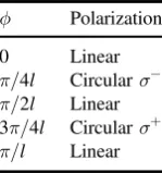
( ) As depicted infigure1, the interference of two
counter-pro-pagating laser beams with mutually orthogonal linear polar-isations results in a total polarisation of left- and right-handed circularity alternately σ+ and σ− at planes separated by an axial distance of λ/4. Between planes the polarisation is linear with polarisation vector pointing at angles±45°. This spatial variation of the wave polarisation along the common axis of the interfering beams constitutes a polarisation gra-dient, which—as will be explained—can lead to a spatially-dependent population differential.
To explain how Sisyphus cooling works, we consider an atom that possesses aJg=1/2 ground state which has only two Zeeman sub-levels g±1/2. Most laser cooling experiments use
optical transitions JgJe=Jg+1, the energy gap between the two states defined as ÿω0. We, therefore, consider a
JgJe=3 2 transition. As in Doppler cooling, we assume red-detuning Δ0<0 where Δ0=(ω −ω0) [43]. The polar-isation gradients created by the interfering counter-propagating beams affect the light shifts and the populations of the atomic
levels which now become spatially dependent. This can be explained as follows. When the atom interacts with a non-resonant lightfield, then in the weak-field limit the ground state levels acquire light shifts U±. Similarly the populations of the
Zeeman sub-levels (for an atom at rest) are now given by
z sin kz
st
1 2 2
P ( ) = ( )andPst1 2 z =cos2 kz
- ( ) ( ), so that these light shifts are spatially dependent and different for the Zeeman sub-levels g±1/2 as illustrated in figure 1. The optical potentials
associated with the two Zeeman sub-level shifts are given by
U 2 kz
3 0 2 cos 2 , 47
= D¢
[ ( )] ( )
where Ω0 is the Rabi frequency. Also, Δ0 and 0
D¢ and the saturation parameters0are given by
s 2; s 2
4. 48
0 0 0 0 0 0 2 2
D¢ = D = W
D + G ( )
Note thatU±are the optical potentials of the ground state
sub-levels∣g1 2ñ. It is easy to see that the minima ofU+correspond
to the maxima of U− and vice versa and the maxima and minima correspond to positions where the polarisation is sˆ
(purely circular).
Early theoretical works which sought to explain the Dop-pler cooling argued that the damping of the atomic gross motion arises from the fact that the atomic internal state does not follow adiabatically the variations of the laser field resulting from atomic motion[60]. Such an effect may be described by a
non-adiabaticity parameterò=vτP/λ=v/(λΓ), defined as the ratio between the distancevτPcovered by the atom with a velocityv during its internal relaxation timeτP(τP=Γ−1), and the laser wavelength. For multi-level atoms, we can similarly define a
non-adiabaticity parameter ¢ =vtP¢ l=v (lG¢). At low
intensities, since G¢G it follows that¢. Thus non-adiabatic effects can appear at much lower velocities(kv» G¢)
than those required by Doppler cooling, and thus can ensure the presence of damping forces even at very low velocities.
Dalibard and Cohen-Tannoudji [58] explained how the damping of the atomic motion is generated. The key point is that, as a condition, the atom must have internal states with energy sub-levels with a strong position-dependence, and which therefore experience large changes as the atom moves. The creation of polarisation gradients can ensure this condi-tion. Let us assume that the atom moves along thez-axis, and it has a speed such that during the optical pumping time
P 1
t = G¢- it travels a distance of the order of the laser wavelengthλ. If the atom starts from the bottom of a valley in a given Zeeman sub-level, then it has sufficient time to reach the top of the hill. At this position, it has a large probability to be optically pumped to the other sub-level and be shifted to the bottom of a valley, and so on: see figure 2. The atom is running uphill more frequently than downhill. This is called a low intensity Sisyphus effect, which arises from the correla-tions between the spatial modulacorrela-tions of light shifts and optical pumping rates. It is important to emphasise the term
‘low intensity’ as the Sisyphus effect we are discussing is valid in the low intensity regime. This is in contrast to another Sisyphus effect which is valid at high intensities, which we shall not discuss any further here [61].
Figure 1.Variations of the populations(spots)and energy level shifts of the ground state sub-levels along thez-axis. Reproduced with permission from[58].
In the process of Sisyphus cooling, an atomic sample eventually reaches an equilibrium temperature. In each optical pumping cycle, we have the emission of afluorescence photon.
Each such photon has an energy higher than the energy of the absorbed photon, by an amount in the order of the light shift∣ ∣.U The excess energy is transferred from the atom to the lightfield leading to a decrease of the atomic energy by the same amount. Repeated pumping cycles, thus, lead to a stepwise decrease of the atomic energy until its total energy is so low that the atom becomes trapped in the optical potential wells associated with the spatially modulated light shifts. The equilibrium temperature of sub-Doppler cooling is therefore expected to be given by:
k T U
4 , 49
B Sis
2 0
0 2 2
» = W D
D + G
∣ ∣ ( )
which for large detuningΔ0?Γtakes the form,
k T U
4 . 50
B Sis
2
0
» = W
D
∣ ∣ ( )
The detailed quantitative treatment of these predictions has been given in[58]. At low intensity, the magnitude of the light shift
U
∣ ∣of the ground state is much smaller than the natural widthÿΓ of the excited state. This explains why it is possible to attain temperatures about two orders of magnitude lower than the Doppler limit, which itself scales asÿΓ. The Sisyphus cooling leads to a damping force which for large detuning is in the form,
FSis= -aFv, aF =k2D0. 51
G ( )
The friction coefficient αF which applies in the case of low intensity Sisyphus cooling, as given in equation (51), is much
larger than the friction coefficient of Doppler cooling: the latter is
of the order of k s2 0
, where the saturation parameters0must be
smaller than one. In typical experiments, both cooling mechan-isms come into play. Although the friction force of the low intensity Sisyphus cooling acts within a much smaller velocity interval than the Doppler cooling, both mechanisms are useful. The Doppler cooling that acts over a relatively large velocity interval drags the atoms towards the velocity region where the Sisyphus cooling operates. Thus, use of the Doppler mechanism as afirst step serves to increase dramatically the number of atoms affected by the sub-Doppler mechanism.
We have seen that the equilibrium temperature is pro-portional to the square of the Rabi frequency, which means that it is directly proportional to the laser intensity. This may incorrectly imply that lowering the intensity can lower the temperature indefinitely. But we must take into account the fact that the scheme is based on spontaneously emitted photons in each pumping cycle. Each photon imparts a recoil momentumÿkto the atom which, according to its direction relative to the atomic motion, may either decrease or increase the atomic kinetic energy. The atomic motion continues to be cooled only so far as the decrease of the total atomic energy due to the Sisyphus effect, remains larger than the increase of the kinetic energy, of the order ofErec, due to recoil associated with the spontaneously emitted photon.
The qualitative description of low intensity Sisyphus cooling, as given above, is based on a classical description of the position of the atomic centre of mass. This means that the moving atom is treated as a classical point particle. This is a reasonable assumption only if the atomic wave packet, which describes quantum mechanically the centre of mass, is well localised in the laser wave. This assumption breaks down when the minimum temperature is achieved and this leads to the conclusion that we must then treat both internal and external variables quantum mechanically. In this case, we can take advantage of the fact that in the Sisyphus effect the motion of the atom occurs in spatially periodic potential wells. This is reminiscent of the electron motion in solid state lattices. Thus, the description of atomic motion could also be given in terms of Bloch states and energy bands [62–64]. In this regime, low intensity Sisyphus cooling is a result of optical pumping processes that accumulates the atoms into the lowest energy bands.
The above arguments may suggest that the photon recoil energyErecshould be the ultimate cooling limit. However, to cool the atomic motion to kinetic energies below the photon recoil energy, atoms with velocity v smaller than the recoil velocityvrecmust be prevented from absorbing light[49,50]. This condition can be satisfied by the creation of atomic dark states for which the fluorescence rate depends on the atomic velocity at the excitation, by a Raman process. When the velocity is zero, or close to zero, the atom does not absorb photons; it thus does not fluoresce, and so it does not experience recoil. We can also use selective Raman processes in which the excitation of the atoms is velocity-selective[65]. However, these mechanisms have basic physical differences from Doppler and Sisyphus cooling. First, the cooling with velocity-dependent dark states is not based on a force. It is Figure 2.When the optical pumping time is sufficiently long, an
atom, initially in theg+1/2Zeeman sub-level, has sufficient time to remain in the position-dependent sub-level which changes in energy (vertical scale)from its value at the bottom of the valley to its value at the top of the hill as the atom moves(from left to right in the
figure). At this position, the atom has a large probability of being optically pumped into the higher state from which it then gets de-excited to the other sub-levelg−1/2at the bottom of the
corresponding valley. This basic set of steps is repeated in each cycle. Reproduced with permission from[58].
rather the result of an inhomogeneous random walk in momentum space which vanishes as the atomic velocity tends to zero. Secondly, in Doppler and Sisyphus cooling the sys-tem reaches a steady state as a result of the competition between the cooling introduced by the friction, and the heating due to fluctuations associated with the random spontaneous emission processes. Such a competition does not exist in sub-recoil cooling.
As a corollary, it is interesting to note why the mech-anism in question is called the Sisyphus effect. The name comes from Sisyphus, a hero of ancient Greek mythology who was punished by Zeus by being forced to transport a heavy rock to the top of a hill. Just before reaching the top, the rock slipped away and rolled downhill to the bottom. The Sisyphus effect is an allusion to his condemnation to repeat this eternally just as the atom loses kinetic energy through transitions involving the potential hills of its space modulated energy levels.
4. Twisted light
Light possessing optical SAM is well known, where optical spin is identified with the intrinsic property of wave polar-isation. The much more recent discovery of twisted light began with the work in 1992 by Allenet al[7]who suggested that it should be possible to generate light beams possessing quantised OAM in the laboratory. The experimental
con-firmation followed soon after, with experiments carried out in a number of laboratories. Research on twisted light continues apace more than three decades later and it has led to funda-mental advances in both concepts and applications (see [1, 66–69]). The most prominent mechanical applications of
twisted light include the optical spanner as the rotational version of the optical tweezer which has also featured in a variety of other applications (see [70–75]). Other
develop-ments involving the application of twisted light include micro-manipulation [76]; quantum communications and cryptography [77–79] and phase contrast imaging (see [80–82]). Twisted light has been presented in some recent
reviews which the reader is referred to, beginning with the 1999 review by Allenet al[1]followed by a number of edited
books, reviews and theme issues (see [66–69, 83]). This
topical review is concerned primarily with the interaction of twisted light with atoms and we feel it is helpful to begin by considering applications involving LG light as the proto-typical form of twisted light. We shall also deal with complex twisted light, which we define as polarised twisted light arising in single or multiple beams and in various geometrical arrangements, including co-propagating or counter-propagat-ing twisted beams with specified wave polarisations in one, two or three dimensional configurations. These sources of
complexity gives rise to novel interactions with atoms in processes involving both the internal and gross atomic degrees of freedom.
4.1. LG light
It is a general feature of twisted light, exemplified by the LG beams, that different modes have helical wavefronts consist-ing of intertwined helices, as shown schematically infigure3.
Modes of the LG type, denoted LGklp, have a wavevector component k along the propagation direction and are char-acterised by the two integer indices: an azimuthal integer indexl, representing the number of intertwined helices and a radial integer index p which arbitrates the number of radial nodes. These directly equate to the degree and order of the associated (generalised) Laguerre polynomial that modifies the Gaussian radial profile. The integer l can be positive or negative, representing two senses of helical wavefront rota-tion. When bothlandpare zero, the mode(k, 0, 0)becomes simply a Gaussian distribution with no angular momentum.
In the paraxial approximation, the electricfield associated with a LG mode, of wavelengthλ=2π/kand frequency ω propagating in thez-direction, and polarised in thex-direction is given by
z t u z e e
E , , , 1 x
2 , , 52
klp(r f )= p∣ ∣l(r ) iQklp(r f, ,z) -i tw ( ) whereup∣ ∣l(r,z)is the amplitude or mode distribution function
u z E C
z z w z
L
w z e
,
1
2
2
53
pl k
l p R
l
p
l w z
00 2 1 2
2
2
2 2 2
r r
r =
+
´ ´ -r
⎛
⎝
⎜ ⎞
⎠ ⎟
⎛ ⎝
⎜ ⎞
⎠ ⎟ ( )
( ) ( )
( ) ( )
∣ ∣ ∣ ∣ ∣ ∣
∣ ∣ ( )
and Θklpis the phase function
z skz l s p l z z
s k z
z z
, , 2 1 tan
2 .
54
klp R
R
1
2
2 2
r f f
r
Q = + - + +
+
+
-( ) ( ∣ ∣ ) ( )
( )
( ) Here Lp∣ ∣l is the associated Laguerre polynomial, w(z)is the beam waist at positionzdefined byw z2( )=2(z2+zR2) kzR, andzRis the Rayleigh range, which is related tow0, the waist
at focus, byzR=pw02 lwhereλthe wavelength of the light. In equation(54), the third term is the Gouy phase for the LG
mode and the fourth term is referred to as the curvature phase term. The factors=±1 takes into account propagation in the opposite directions along the±z-axes, while the factorC∣ ∣l pis given byC∣ ∣l p= 2p! p(∣ ∣!l +p!).
An important feature of all twisted light fields is the existence of the phase factor eilf. However, the full phase Θklp(ρ, f, z) is essential for describing the various effects including rotational effects when the light interacts with atoms and molecules. Figure 3shows by way of an example the characteristic features of optical vortex beams concerning phase variations and helical wavefronts.
A LG beam characterised by the electricfieldEklp(ρ,f,z) has a linear momentum ÿkand carries an angular momentum equal to lÿ per photon. The quantum number l is called the winding number(or the topological charge)and we re-emphasise
that l can take both negative and positive integer values, corresponding to right-hand and left-hand twisting of the
wavefront. LG modes for which l¹0 but p=0 are called donut modes, since the light intensity is ring-shaped as shown
figure4for the casesl=1 andl=3. Figure4also shows the case of a double ring mode arising whenl=1,p=1.
It is often sufficient to focus on the form of twisted light without explicit details of the LG form. An electromagnetic light mode of frequencyωand OAMlÿpossesses an electric field vector distribution which can be written in cylindrical polar coordinatesr=(r,z)as follows
t F e e
E r, 1
2 , 55
kl( )= ˆ ( )r i kz( -wt) ilf ( ) whereˆ is a wave polarisation vector andF(ρ)is a scalar dis-tribution function which depends only on the radial coordinateρ. Note that, unless a paraxial approximation is deployed, the polarisation vector need not necessarily reside in the plane represented byr. Thefield in equation(55)emerges from the familiar LG light distribution in the limit of large Rayleigh range
zR ¥, a situation which is often encountered and is realisable in practice. This simplified form offield is advantageous for a
number of reasons. It has the desired feature in being endowed with OAM, by virtue of the azimuthal phase factor, and is free from the curvature problems which often distract from the fundamental issues involving OAM of light in a real LG beam, i.e. with afinite Rayleigh range.
4.2. Other types of twisted light—Bessel beams
Besides the LG beam, a second, somewhat simpler, type of vortex beam is the Bessel beam[84]. This is characterised by
a transverse electric field which is also a solution to the electromagnetic vector Helmholtz equation, with the modes characterised by only one integer number l, that can take either positive or negative values. We have in cylindrical polar coordinates r=(ρ,f,z)
t E J k e e e
E r( , )=eˆ 0l l(^r) ikz ilf -i tw, ( )56 whereE0lis the amplitude and the unit vectoreˆ designates a wave polarisation. The radial function Jl(k⊥ρ) is the Bessel
[image:14.595.115.486.76.318.2]function of orderl where, as in LG beams,lis the winding number and the vortex beam carrieslÿOAM per photon. The Figure 3.Left: continuous phase ramps in transverse planes perpendicular to the beam axis forl=1(left, top)andl=3(left, bottom). Here, colours through the spectrum denote the optical phase, repeating on a 2πinterval with an arbitrary zero. Right: thel=3 three-part wavefront, a helical surface of constant phase.
Figure 4.The intensity distributions of modes, respectively, for LG1,0(donut mode), LG3,0(donut mode)and LG1,1(two-ring). These radial intensity distributions are at the waist planez=0. The insets exhibit graphically the corresponding radial intensity distributions with radial distance in units of wavelength.