Imaging of a Distinctive Large Bubble in Gas-water Horizontal Flow Based on Size Projection Algorithm

777

Imaging of a Distinctive Large Bubble in Gas-water Horizontal Flow

Based on Size Projection Algorithm

K. Li1,2_{, Q. Wang}2_{, M. Wang}2*_{, N. Yang}1_{, Y. Han}1

1_{Shanxi Key Laboratory of Signal Capturing and Processing, North University of China, Taiyuan,}

030051, China

2_{School of Chemical and Process Engineering, University of Leeds, Leeds, LS2 9JT, UK}

*_{Email: [email protected]}

ABSTRACT

Electrical resistance tomography was succeed in being applied on gas-liquid two-phase flow, but it is incapable on determination of sharp interfaces between gas and water, which impedes effective estimation of fluid characteristics and flow regimes. Thresholding value method was demonstrated an abstractive view of most flow regimes, particularly a large bubble with a shape intermedium boundary. In principle, the thresholding values should be based on bubble merging principles, but is determined empirically in most practices, which may present a challenge in correctness. In this paper, a size projection algorithm is proposed for imaging a large bubble with distinctive boundary by searching an optimal thresholding value, which may provide a better estimation of the bubble size. Results from experiments engaged with typical gas-liquid flow regimes, including stratified, plug, slug and annular flow regimes, with large air cavity in a 50mm-diameter horizontal pipeline are reported in the paper, which especially focuses on imaging of the size of large bubble with the proposed method. The results are also compared with the images obtained from wire-mesh sensor system and videos taken from a transparent section of the test rig.

Keywords Electrical resistance tomography, gas-water flow visualisation, Distinctive large bubble, Size projection algorithm

Industrial Application General

1 INTRODUCTION

Gas-water two-phase flows are a common and important transportation in many industries, where measuring of flow parameters for understanding flow dynamics in process equipment is of significance for operation, analysis and design of these equipment (Levy, 1999; and Wang, 2015). Due to electrical resistance tomography (ERT) providing a non-intrusive and cost-effective solution with a high temporal resolution (sub-millisecond) (Wang, 2005), it was succeed in being applied on gas-water two-phase flow measurement and visualisation. However, with a relative low spatial resolution (up to 5%) (Wang, 2015), it is normally incapable for determination of sharp interfaces between two phases, which impedes effectively characterizing and visualising of gas-water two phase flows.

Thresholding value methods were successfully applied to enhance the effectiveness of visualisation for gas-in-water flow, which demonstrated an abstractive view of most flow regimes can be displayed, particularly for a distinctive large bubble with a shape intermedium boundary. Wang (1995, 2017) used thresholding value to extract the objects size in testing field based on engineering experience. Xie et al (1992) used the proportion of reconstructed mean value as thresholding value, and Kim et al (2011) chose a histogram of reconstructed image as the criterion to select the thresholding value, which were all based on reconstructed tomogram. However, these methods still left the selection of the thresholding value as trial-and-error in practice. It is known that a fixed thresholding value would not be optimal since characteristics of fluids, and flow rigs and condition under operation are hardly same (Glasbey, 1993).

778

large bubble with few small bubbles in its tail (e.g. slug or plug regimes). According to general flow principle (Levy, 1999; Razzaque, 2005), the large bubble was main part in determining void fraction. We understood that the large bubble, if it exists, plays a dominant role in tomography imaging, and the influence from small bubbles is mostly depressed in the tomogram since they were normally few accompanied with a large bubble in these typical flow regimes. With the ignoring of small bubbles, the size projection-based algorithm was proposed for accurately extracting the interface between gas and water, which might enhance the visualisation performance of distinctive bubble in stated flow cases of (2) and (3). The paper demonstrates results from visualisation of typical flow regimes in a 50mm-diameter horizontal pipeline, including stratified, plug, slug and annular flow regimes. The results were also compared with videos taken from a transparent section and images obtained from wire-mesh sensor (WMS) system.

2 METHOD

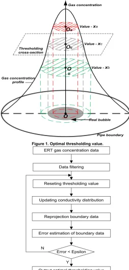
Conventionally, the thresholding value used to enhance tomographic flow visualisation is a fixed global value from flow engineering experience or a histogram of reconstructed images (Wang, 1995 & 2017; Xie, 1992; Kim, 2011), which is considered not optimal for dynamic change of flow condition. The principle of the size projection method, based on original measured boundary data, is proposed to accurately estimate the projected size of bubble by projecting the automatically searched optimal thresholding value.

2.1 Size Projection Algorithm

Since EIT system can manage near-full void fraction range (close to 100%) for gas-water two phase flow (Jia, et al 2015), the bubble size and shape might be accurately extracted from gas concentration tomogram if an optimal thresholding value

x

c, as shown in Figure 1 known, where thrsholding value

a

x

and

x

bunderestimated and overestimated bubble size respectively. With the assumption, the

method of automatically adjusting thresholding value is presented below, which is based on error-minimisation of boundary data between boundary voltages acquired from ERT sensor and computed from a projected conductivity distribution using the size projection method. The procedures of the method is shown in Figure 2.

Because of the unavoidable noise in measurement, the gas concentration data obtained from ERT system might contain few abnormal data, e.g. beyond real meaningful volumetric range [0.0, 1.0], which should be filtered with Equation (1).

n

i

i

c

i

c

i

c

i

c

i

C

,

1

...

1

)

(

0

.

1

1

)

(

0

)

(

0

)

(

0

.

0

)

(

=

⎪

⎩

⎪

⎨

⎧

≥

<

<

≤

=

(1)

779

Value - xa

Oa

Oc

O b

O

Gas concentration

Value - xc

Value - xb

Real bubble

Pipe boundary Thresholding

cross-section

[image:3.595.179.433.72.604.2]

Gas concentration profile

Figure 1. Optimal thresholding value.

ERT gas concentration data

Data filtering

Reseting thresholding value

Updating conductivity distribution

Reprojection boundary data

Error estimation of boundary data

Error < Epsilon

Output optimal thresholding value Y

N

Figure 2. Flow chart for size projection algorithm.

As a concentration tomogram represents the gas distribution in the cross-section of pipeline flow, thresholding method is used to extract the gas-water interface, where the low concentration region denotes the water phase and the high concentration region denotes gas phase. Once the thresholding value is adjusted, the binary conductivity distribution for the forward solution computation will be updated with following Equation (2).

⎪⎩

⎪

⎨

⎧

≥

<

=

_{( )}

) ( )

(

)

(

)

(

)

(

_n

g

n w

n

x

i

C

x

i

C

i

σ

σ

780

where,

σ

(n)is the

n

-step updated conductivity vector,

σ

_wand

σ

_gare the water conductivity and gas conductivity respectively,

x

(n)is the thresholding value in respect to the

n

-step.

The ERT forward solution is employed for computing the boundary voltage vector and producing an error vector of boundary data between acquired from measurement and computed with the updated conductivity distribution, which is expressed as Equation (3) (Wang, 2002).

)

(

)

(

)

(

)

(

) 0 ( ) ( ) (

σ

σ

σ

σ

u

u

V

V

e

n

₌

ʹ

ʹ

₋

ʹ

n ₍₃₎

where,

e

(n)is the

n

-step boundary data error,

V

(

σ

)

and

V

ʹ

(

σ

ʹ

)

are the measured reference voltage and measurement voltage respectively,

u

(

σ

(0)

)

and

u

ʹ

(

σ

(n)

)

are computed reference voltage in respect to the initial conductivity estimation and measurement voltage in respect to the

n

-step updated conductivity vector

σ

(n).

With the automatically adjusted thresholding value, the binary conductivity distribution (i.e. gas cavity in water with a sharp interface) is projected and then, the boundary data error is updating until reaching to an acceptable value. As shown in Figure 1, the automatic search should be converged since the error is minimised only as the optimal thresholding value is approaching to the real bubble, while the boundary voltage error must become bigger as the thresholding value overestimated or underestimated. For a full range of gas concentration, the error is a quadratic function of thresholding value, whose minimum almost reaches 0 (i.e. the relative change of computed data is close to measured data, and the updated binary distribution is close to real distribution).

Given a definition interval in respect to gas concentration, an error function of thresholding value is defined as:

]

0

.

1,

0

.

0

[

)

(

∈

=

F

x

x

e

(4)

where,

F

(

x

)

maps thresholding value

x

to boundary data error

e

. According to the procedures of the size projection algorithm, the error function is a single peak in definition interval. The golden-section search method is applied to optimise the search for error minimisation and determination of the optimal thresholding value projected in each tomogram. After obtaining the optimal thresholding values, the gas concentration of each tomogram can be updated with following the assumption, where pixels with value higher than the optimal value are fully occupied by gas, and pixels with lower concentration are fully occupied by water. The gas-water interfaces can then be extracted and the large bubble distribution can be accurately obtained.

2.2 Experiments setup

[image:5.595.92.543.67.317.2]

781

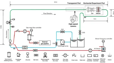
Figure 3. Sketch of experimental facility.

2.3 Data processing

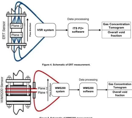
As shown in Figure 4, the ERT measurement data were collected by v5r system (Jia, et al 2010) with a data acquisition speed being configured as 312.5 dual-frames per second, and ITS p2+ software (ITS plc, 2010) was used to extracted gas concentration tomogram and overall void fraction. The v5r system, a voltage-drive ERT system, performed well for horizontal flow regimes (Jia, et al 2015). The sensitivity coefficient back-projection (SBP) algorithm (Wang, 2002) was used to convert the relative voltage change to conductivity distribution, then the gas concentration of each pixel was derived from conductivity based on Maxwell relationship. Since gas-water in two phases flow are immiscible and gas conductivity is zero in the experiments, the relationship is simplified as Equation (5).

1 1 1 1

2

2

2

2

2

2

σ

σ

σ

σ

σ

σ

σ

σ

mc mc mc mc

c

+

−

=

+

−

=

(5)

where,

c

is gas concentration (i.e. void fraction),

σ

1 is the conductivity of continuous phase (water),

mc

σ

is reconstructed local conductivity, and

σ

1

/

σ

_mcis conductivity ratio obtained from SBP. The overall void fraction

α

was derived from the average of gas concentration in each pixel.

Applying the size projection algorithm introduced in former section 2.1, the optimal thresholding value

opt

x

for each frame was accurately determined. Then, the projected gas concentration with optimal thresholding value was updated with following Equation (6). The overall void fraction

α

of size projection algorithm was derived from the average of projected gas concentration in each pixel.

⎩

⎨

⎧

<

≥

=

ʹ

opt opt

x

i

C

x

i

C

i

C

)

(

0

.

0

)

(

0

.

1

)

782

Fl

ow

d

ire

ct

io

n

V5R system _softwareITS P2+

Gas Concentration Tomogram Overall void

[image:6.595.64.502.73.464.2]

fraction Data processing

Figure 4. Schematic of ERT measurement.

Fl

ow

d

ir

ec

tio

n

WMS200

system WMS200 software

Data processing

Gas Concentration Tomogram Overall void

fraction

Figure 5. Schematic of WMS200 measurement.

Meanwhile, the WMS200 measurement data were collected simultaneously with the speed being configured as 5000 dual-frames per second, and WMS200 software was used to produced gas concentration tomogram and overall void fraction (Beyer, 2012), as shown in Figure 5. The local void fraction of

i

th crossing point was calculated by Equation (7) and the overall void fraction was derived by Equation (8) according to the different area occupied by each crossing point.

w meas w

U

U

U

i

)

=

−

(

α

(7)

∑

⋅

=

i

p

i

i

)

(

)

(

α

α

(8)

where,

α

(i

)

is the void fraction of

i

th crossing point,

U

_wand

U

_measrepresent the sensor signal of calibration value (tap water) and measured value, respectively. α is the overall void fraction,

p

(i

)

is the weighting coefficient which denotes the proportion of the area occupied by the

i

th crossing point to the total area of the pipe.

783

[image:7.595.100.527.71.290.2]

(a) ERT pixels distribution (b) WMS200 crossing points distribution

Figure 6. The pixel distribution and crossing point distribution of cross-section

3 RESULTS AND DISCUSSION

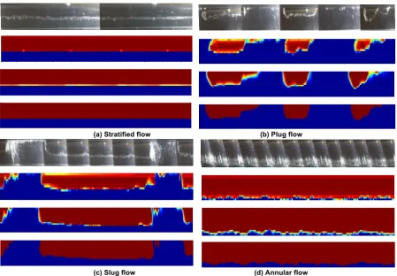
As the ERT sensor (non-intrusive) was installed in the front of the wire-mesh sensor (intrusive) in the horizontal pipline towards the flow and they were also closer to each other with 20cm-distance on the pipeline, the flow condition and resultant flow regimes should be assumed in a high consistency. For typical horizontal flow regimes, covering stratified, plug, slug, and annular regimes, the axial stacked images obtained from different methods were compared, as shown in Figure 7. From Figure 7(a)-(d), all images from ERT reconstruction consist of 625 frames (i.e. time length is 2s), and all images from WMS200 consist of 10000 frames with same time length.

Figure 7(a) shows four images of bubble regime with a superficial liquid velocity of 0.1 m/s and superficial gas velocity of 0.2 m/s. The first image recorded with the high-speed camera shows the gas and water separately flowing with few small bubbles at the gas-water interface. The second image obtained with WMS200 and the third image reconstructed with ERT shows the same results, while the fourth image projected from ERT reconstruction with the size projection algorithm only shows the horizontal gas-water interface without any small bubbles.

Figure 7(b) shows four images of plug regime with a superficial liquid velocity of 1.0 m/s and superficial gas velocity of 0.2 m/s. The first camera image shows the gas phase is deformed in to large bubbles (i.e. gas plugs) and water is distributed at the bottom of the pipeline or between gas plugs with some small bubbles inside. The second WMS200 image and the third ERT image show similar results, with few small bubbles at the tails of gas plugs. The fourth image shows a clear gas-water interface, and the existence of the small bubbles is ignored.

Figure 7(c) shows four images of slug regime with a superficial liquid velocity of 0.2 m/s and superficial gas velocity of 2.0 m/s. The first image shows the large gas slugs almost occupy the pipeline with separated by water and many small bubbles exist at the tails of gas slugs. The second WMS200 image and the third ERT image show similar results, but combine small bubbles at slug tail into large bubble. The reason might be too much small bubbles resulted in a high gas concentration in the pixel or crossing points. The forth image shows clear gas-water interface of slug bubbles, and combine small bubbles into large bubble, as well, since size projection algorithm based on ERT reconstructed gas concentration.

784

gas-water interface, but it does not show the thin film of water at top. The reason is too thin film of water on the wall of pipe cannot be identified by ERT with SBP reconstruction algorithm. The fourth image shows clear gas-water interface with ignoring the existence of small bubbles on it, and also does not show the thin film of water at top, as well, since size projection algorithm based on ERT reconstructed gas concentration.

(a) Stratified flow (b) Plug flow

[image:8.595.59.509.141.453.2]

(c) Slug flow (d) Annular flow

Figure 7. Axial stacked images of gas-water flow (flow direction from right to left) by different methods. ( Images from the top to bottom of columns are from: video of high-speed camera; wire-mesh sensor; ERT normal

image; ERT image reconstructed with the size projection algorithm.)

4 CONCLUSION

A size projection algorithm is presented for enhancing the visualisation of gas-water horizontal flows, especially for imaging of a distinctive large bubble. The results were compared with the images, including stratified, plug, slug and annular regimes in a 50mm-diameter horizontal pipeline, obtained from a videos camera, wire-mesh sensor system, conventional ERT and the size projection algorithm. The following conclusions can be drawn from the study:

• The size projection algorithm performs well to extract the gas-water interface with ignoring

small bubbles, which shows a clear boundary between two phases and makes it possible to accurately estimate the size and shape changing of bubbles.

• It is hard to identify small bubbles in high concentration, such as at the tails of gas slugs, since

the spatial resolution is an unavoidable limitation.

• The performance of WMS200 and ERT with SBP algorithm are kept a high consistency, while

ERT does not performs as well as WMS200 for annular flow regime since it cannot identify the thin film of water at the top of the pipe.

• It would be worthy to carry out 3D visualisation with size projection algorithm to show the

veritable large bubbles in gas-water flow.

•

785

ACKNOWLEDGEMENTS

The authors would like to express their gratitude for the support from the Chinese Scholarship Council (CSC) and the School of Chemical and Process Engineering, who made Mr. Li’s study at the University of Leeds possible.

REFERENCES

BEYER M, SZALINSKI L, SCHLEICHER E, (2012) Wire-Mesh Sensor Data Processing Software User Manual and Software Description, Version 01.02.2012

GLASBEY C. A, (1993) An analysis of histogram-based thresholding algorithms. Academic Press, Inc. HEWITT G.F, HALL-TAYLOR N.S, (1970) Annular two-phase flow, Pergamon press, ISBN: 0080157971

Industrial Tomography Systems LTD, (2010) ITS P2+ Electrical Resistance Tomography System - Users Manual, Version 7.0. Manchester: Industrial Tomography Systems Ltd.

JIA J, WANG M, SCHLABERG H. I, LI H, (2010) A novel tomographic sensing system for high electrically conductive multiphase flow measurement. Flow Measurement & Instrumentation, 21(3), 184-190.

JIA J, WANG M, & FARAJ Y. (2015) Evaluation of EIT systems and algorithms for handling full void fraction range in two-phase flow measurement. Measurement Science & Technology, 26(1). DOI: 10.1088/0957-0233/26/1/015305

KIM, B. S, KHAMBAMPATI A. K, (2011). Image reconstruction with an adaptive threshold technique in electrical resistance tomography. Measurement Science & Technology, 22(10), 880-897.

LEVY S, (ed) (1999) Two-phase flow in complex system, John Wiley & Sons, ISBN: 0-471-32967-3

RAZZAQUE, M M, (2005) Bubble size distribution in a large diameter pipeline. Proceeding of IMEC & APM, Dhaka

WANG M, DICKIN F. J, & WILLIAMS R. A. (1995) A Study on Cyclonic Separators Using Electrical Impedance Tomography. Proceeding of Multiphase Flow, Kyoto

WANG M, (ed) (2015) Industrial Tomography - Systems and Applications, Elsevier, ISBN: 978-1-78242-118-4.

WANG M, (2002), Inverse solutions for electrical impedance tomography based on conjugate gradients methods. Measurement Science & Technology, 13(1), 101.

WANG M, MA Y, HOLLIDAY N, DAI Y, WILLIAMS R. A, & LUCAS G, (2005), A high-performance EIT system. IEEE Sensors Journal, 5(2), 289-299; DOI: 10.1109/JSEN.2005.843904

WANG Q, (2017), A Data Fusion and Visualisation Platform for Multi-Phase Flow by Electrical Tomography, PhD thesis, University of Leeds.