A composite Bayesian hierarchical model of compositional data with zeros

This is a repository copy of

A composite Bayesian hierarchical model of compositional

data with zeros

.

White Rose Research Online URL for this paper:

http://eprints.whiterose.ac.uk/100013/

Version: Accepted Version

Article:

Napier, Gary, Neocleous, Tereza and Nobile, Agostino orcid.org/0000-0002-5344-8525

(2015) A composite Bayesian hierarchical model of compositional data with zeros. Journal

of Chemometrics. 96 - 108. ISSN 1099-128X

https://doi.org/10.1002/cem.2681

Reuse

Items deposited in White Rose Research Online are protected by copyright, with all rights reserved unless indicated otherwise. They may be downloaded and/or printed for private study, or other acts as permitted by national copyright laws. The publisher or other rights holders may allow further reproduction and re-use of the full text version. This is indicated by the licence information on the White Rose Research Online record for the item.

Takedown

If you consider content in White Rose Research Online to be in breach of UK law, please notify us by

A composite Bayesian hierarchical model of

compositional data with zeros

Gary Napier∗ Tereza Neocleous∗ Agostino Nobile††

September 26, 2014

Abstract

We present an effective approach for modelling compositional data

with large concentrations of zeros and several levels of variation,

ap-plied to a database of elemental compositions of forensic glass of

vari-ous use types. The procedure consists of: (i) partitioning the data set

in subsets characterised by the same pattern of presence/absence of

chemical elements and (ii) fitting a Bayesian hierarchical model to the

transformed compositions in each data subset. We derive expressions

for the posterior predictive probability that newly observed fragments

of glass are of a certain use type and for computing the evidential value

of glass fragments relating to two competing propositions about their

source. The model is assessed using cross-validation, and it performs

well in both the classification and evidence evaluation tasks.

Keywords: Bayes factor; classification; evidence evaluation;

foren-sic glass; Markov chain Monte Carlo

1

Introduction

Chemical compositions often contain large concentrations of zeros, which

require special consideration during the statistical modelling process. We

focus on the elemental composition of glass and construct a model that deals

with this data complexity in a practical way. The elemental composition

data, described in detail in Section 2, consist of the percentage weights

(wt%) of each chemical element comprising a glass fragment. They contain

many zeros indicating that an element is either below limits of detection

or absent from the composition of a fragment. Our model accounts for the

presence (above limits of detection) or absence (below limits of detection)

of particular elements, and seems to improve performance in tasks related

to the statistical analysis of glass fragments in a forensic context.

Analysis of glass fragments for forensic purposes usually focuses on evidence

evaluation, which relates to the comparison of two sets of fragments under

competing propositions, or, at the investigation stage, on the classification

of a fragment into a use-type category (type of glass object from which the

fragments could have originated). Most glass fragments analysed by forensic

experts are too small for their use type to be determined by their thickness

or colour [1], so measurements of physico-chemical features of the fragments,

such as the refractive index or elemental composition, are obtained. Such

measurements are also used for computing a numerical measure of the

evi-dential value of glass fragments transferred to or from a crime scene.

In this paper we present a model that allows us to address both evidence

evaluation and classification of glass fragments, while dealing with the issue

combines models on lower-dimensional subsets of the data, which are

de-termined by presence/absence patterns of the elements iron and potassium,

and performs well in simulation studies to assess classification and evidence

evaluation performance.

The paper is organised as follows: the glass data set and data

transforma-tions applied to it are described in Section2. Section3presents the approach

to handling compositional zeros and Section4 describes the Bayesian

hier-archical model for the forensic glass data. Section 5 gives details of how

the composite model is put together and describes how the model is used to

classify glass items into use-type categories. Section6discusses the evidence

evaluation procedure. Concluding remarks are provided in Section 7.

2

Glass data

The data were provided by the Institute of Forensic Research, Krakow, and

were collected in an experimental setting. Glass fragments from 320 glass

objects of five use types (26 bulbs, 94 car windows, 16 headlamps, 79

contain-ers and 105 building windows) were analysed. Their elemental content was

measured using a scanning electron microscope with an energy-dispersive

X-ray (SEM-EDX) spectrometer [1]. SEM-EDX produces measurements on

the percentage weight (wt%) of the main elements making up the

compo-sition of the glass items. These are oxygen (O), sodium (Na), magnesium

(Mg), aluminium (Al), silicon (Si), potassium (K), calcium (Ca) and iron

(Fe). Three replicate measurements were taken on four glass fragments from

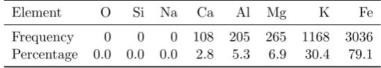
The data are compositional: the percentage weights of each fragment are

non-negative and sum to 100%. Some of the percentage weights are zero;

the frequency of zeros for each element is shown in Table1.

Table1about here.

Denoting the number of elements in the composition byD, the percentage

weights w = (w1, . . . , wD) satisfy PDd=1wd = 100 and wd ≥ 0 and can be

transformed by taking the ratio ofD−1 elements to the remaining one. This

removes the issue of the constrained sample space and reduces the dimension

of the data vector toD−1. The transformed vector is

w∗ =

w1

wD

, . . . ,wD−1 wD

, (1)

where oxygen (O) was chosen as the common divisor, wD, because it is

always present in glass and has the highest weight percentage.

While the Dirichlet distribution would seem a natural fit to modelling

com-positional data, it is restrictive in a way that prevents it from detecting

correlation between subcompositions from the same full composition; this

is referred to as complete subcompositional independence [2, Chapter 10].

Instead, a data transformation is typically applied to (1) to achieve

vari-ance stability and normality. The most common choice of transformation

for compositional data is the additive log-ratio (ALR) of Aitchison [2] which

takes the logarithm of (1). Other transformations that have been applied

to compositional data include the Box-Cox [3], isometric log-ratio [4],

hy-perspherical [5, 6, 7], centred log-ratio [8], multiplicative log-ratio [9] and

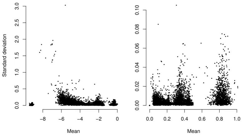
Some members of the Box-Cox family of transformations were examined,

with improvements in variance stability and normality of the data obtained

by applying the square root transformation to (1). A comparison of the ALR

and square root transformations can be seen in Figure1and shows that the

square root transformation is more effective at stabilising the variability

in the data. Furthermore, the square root transformation can be applied

directly to compositional zeros, while logarithmic transformations require

replacing them by a small constant (see Section 3). For these reasons, the

square root transformation was considered the appropriate choice for the

analysis of these data.

Figure1 about here.

3

Compositional zeros

There are two types of compositional zeros: rounded zeros, indicating that if

present a component is below some detection limit, and essential zeros,

de-noting the absolute absence of a component from an observation [12].

Com-positional zeros in glass are most often treated as rounded zeros under the

assumption that traces of certain elements are present but below detection.

The simplest strategy then is to replace rounded zeros by some small

con-stant equal to or below the detection limit. Techniques for doing this include

the additive replacement strategy of Aitchison [2] and the multiplicative

re-placement strategy of Mart´ın-Fern´andez et al. [13]. Palarea-Albaladejo et

al. [14] introduced a parametric approach that reduces artificial correlation

induced by such strategies. For the case of essential zeros Butler and

mass at zero; see also [16].

Here, we partition the glass data depending on whether the elements iron

and potassium are present (above the detection limit) or absent (below the

detection limit) from each composition. Any (D−1) dimensional

compo-sition (1) with Z zero elements is reduced to a (D−Z −1) dimensional

subcomposition, by simply removing the zeros. A separate model is then

estimated for each resulting subset of the data. In fact, Stewart and Field

[9] handled zeros in a similar way by proposing a mixture model that splits

the data according to the presence or absence of components.

Observing the presence or absence of an element from the composition of

a glass item can help determine its use type. For example, none of the

bulbs and headlamps in our database contain iron; therefore, a composition

containing iron is thought as being unlikely to be of either of these types.

Other techniques of obtaining the elemental composition of glass fragments,

such as laser ablation inductively coupled plasma mass spectrometry, may

detect traces of such elements in these glass types [17]. Oxygen, silicon

and sodium are always present in glass. The remaining five elements could

be present or absent, giving 32 possible presence/absence configurations.

Only 10 of these configurations were found in the glass database, with most

accounting for very few items. In fact, as can be seen in Table 1, iron

and potassium are responsible for 87.9% of zero measurements, thus only

focusing on the presence or absence of those two elements allows for the

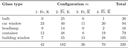
majority of zeros to be removed from the data. We therefore consider only

four configurations as shown in Table2.

Typically, the presence or absence of an element in a glass item is

unam-biguous: out of 320 items, only eight have a chemical element with its 12

measurements not all positive or all zero. In general, we assumed that an

element is present in an item if at least one of its 12 measurements is positive.

Modelling of nonzero subcompositions reduces the biasing influence of zeros

on the distribution of the data. This is shown in Figures2and3, containing

plots of the item means for the whole data set, and for the subset having

configuration 2 (Fe, K) from Table2. In Figure 3, an improvement can be

seen in the symmetry and concentration of points once the large mass at

zero for iron is removed.

The next section discusses a Bayesian hierarchical model for the glass data.

A separate model is estimated for each subset of the data with a given

pattern of presence/absence of chemical elements, which we call elemental

configuration. We consider four models, one for each configuration m =

1, . . . , M = 4 reported in Table2.

Figure2 about here.

Figure3 about here.

4

Bayesian hierarchical model

Aitken and Lucy [18] and Neocleous et al. [10] used frequentist approaches

to modelling the elemental composition of glass fragments using random

effects models with two levels of variation: between-item and within-item.

the data using a mixed effects model. The model contains a fixed effect for

the mean by glass type, and three random effects: at item level, at fragment

level and at measurement level.

For each data set with a given elemental configuration m (often not

ex-plicitly indicated), we denote by ztijk the p-vector of square roots of the

compositional ratios from thek-th measurement on the j-th fragment from

thei-th item of use typet, and assume that

ztijk =θt+bti+ctij+ǫtijk,

btiiid∼Np(0,Ωt−1), ctij iid∼Np(0,Ψ−1), ǫtijk iid∼Np(0,Λ−1).

(2)

The parameter θt is the mean vector for use type t; bti is the item-level

random effect; ctij is the fragment within item random effect; and ǫtijk

denotes the measurement error. Multivariate normal distributions are

as-sumed for all random effects, with unknown precision matrices, Ωt, Ψ and

Λ. The dimensionpmay differ across elemental configurations. The

param-eters in the model are collectively designated as ξm = {θ,Ω,Ψ,Λ}, where

θ={θt}Tt=1 and Ω ={Ωt}Tt=1; for the random effects we use the shorthands

b={bti}I_i=1t Tt=1 and c ={ctij}J_j=1 I_i=1t Tt=1. The symbol T = 5 denotes the

number of use types;Itis the number of glass items of use type t(I1= 26,

I2 = 94,I3 = 16,I4 = 79,I5 = 105);J = 4 is the number of fragments from

each item; andK= 3 is the number of repeated measurements on each

frag-ment. If we denote byztheJKmeasurements on an item of use typeTz=t,

then model (2) implies that the distribution of z, without conditioning on

the random effects, is

where the covariance matrix Σt is given by

Σt= (1J K1′J K)⊗Ω−t1+

IJ ⊗(1K1′K)

⊗Ψ−1+IJ K⊗Λ−1, (4)

1d denotes a column vector of d1’s, andId is thed×didentity matrix.

The prior distributions on the fixed effectsθt are independent multivariate

normals truncated to the positive orthant, to ensure that the means for the

square-root-transformed data are non-negative:

θt iid

∼Np(0,Φ−1), θt>0, t= 1, . . . , T.

The covariance matrix Φ−1 is fixed and equal to s·Ip, with s a relatively

large constant, we used s= 1000. Conjugate Wishart priors are placed on

the precision matrices of the random effects:

Ωt∼Wp(d1t, At), Ψ∼Wp(d2, B), Λ∼Wp(d3, C),

where the degrees of freedom d1t, d2 and d3 are all set equal to p, and the

precision matrices At, B and C are set to (1/1000)·Ip. It was necessary

to introduce separate precision matrices, Ωt, for each glass type, due to the

random variation between items having different properties across use types,

as can be seen from the results in Section4.2.

4.1 MCMC implementation

Markov chain Monte Carlo (MCMC) methods are used to sample from the

joint posterior distribution of the parameters in the model,ξm ={θ,Ω,Ψ,Λ}

quantities are standard distributions and are reported in Appendix A.1.

These are used to update b, c, Ω, Ψ and Λ, using Gibbs sampling moves;

see [19] for an introduction to Gibbs sampling. The update ofθtis performed

by means of a Metropolis-Hastings (M-H) move, with proposal distribution

equal to the multivariate normal in the full conditional distribution of θt,

disregarding the restriction to the positive orthant. The acceptance

prob-ability is either 1 or 0, depending on whether the candidate vector falls in

the positive orthant or not.

We also use two additional M-H moves to update the θt’s. The first one is

performed on θ1 only, as the samples for this vector displayed appreciable

positive autocorrelation. It is a random walk M-H move, performed on each

element ofθ1 separately, with uniform proposal over an interval centred at

the current value, and with interval widths determined from a preliminary

run.

The second move changes at onceθ and b, with the candidate state chosen

in a way that leaves the likelihood unchanged. This move is a special case of

the M-H algorithm as described in [20]. It is discussed in detail in appendix

A.2and, in our experiments, it substantially reduced autocorrelation of the

samples.

4.2 Posterior samples for configuration m= 2 (Fe, K)

The results shown are those for items with configurationm= 2 (Fe, K) from

Table2. Similar results for the three other configurations are not reported

here. All of the analysis was carried out using the statistical programming

approximately 10 hours, which included a burn-in period of 10,000, and also

thinning of the Markov chain, where every 200th _{draw was stored and the}

rest discarded. The acceptance rate for the M-H move performed onθ1only

was 31%, and the rate for the joint move onθ and bwas 54%. Time series

plots of the sampled fixed effect θt are shown in Figure 4. Scatterplots of

the draws of θt are displayed in Figure 5 and show clear separation in the

means between the five use-type categories.

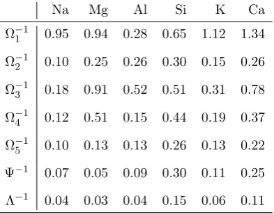
As can be seen in Table3, the variability at item level is shown to be rather

different between use types, which is why the model accommodates for these

differences by allowing the covariance matrix at item level, Ω−_t1, to change by use type. When we compare the variability at fragment level, Ψ−1_{, with}

that for the measurement error, Λ−1, there is little difference observed, with the variability at fragment level being slightly greater, as would be expected.

As expected the variability between glass items is much greater than that

found within items.

Table3about here.

Figure4 about here.

Figure5 about here.

5

Composite model

In the previous section we specified multivariate mixed effects models for the

square-root-transformed compositions z, one model for each configuration

we show how these configuration-specific models can be pulled together in a

single model. The model is then used in section5.1to compute the use-type

probabilities for a newly observed item y of unknown use type. We begin

with some definitions.

Let D = {zti, i = 1, . . . , It, t = 1, . . . , T} be the reference data, where the

numbersItof items of use typetare under control of the experimenter. Also

letDm ={z∈D:Cz=m}be the subset ofDwith elemental configuration

m. For any given z ∈ D, the hierarchical model (2) for configuration m

supplies the distribution

p(z|Tz=t,Cz=m, ξ) =p(z|Tz=t,Cz=m, ξm)

whereξ ={ξm}Mm=1 denotes the collection of parameters across all

configu-rations. More specifically, p(z|Tz =t,Cz=m, ξm) is given by formulae (3)

and (4).

Letϕt= (ϕt1, . . . , ϕtM) be an unknown vector of configuration probabilities

for an itemz of use typet:

ϕtm = p(Cz=m|Tz=t, ϕ, ξ) = p(Cz=m|Tz=t, ϕt). (5)

We assume that a priori the configuration probabilities ϕ = {ϕt}Tt=1 are

independent ofξ and have independent Dirichlet prior distributions:

ϕt|ξ ∼ Dir(αt1, . . . , αtM), t= 1, . . . , T, (6)

where theαtm’s are suitable constants reflecting any prior information about

details on the choice of theα’s.

Next we derive the likelihood function L(ξ, ϕ). The distribution of a single

itemz∈D, given its type Tzand the parameters ξ and ϕ, is

p(z|Tz=t, ξ, ϕ) = M

X

r=1

p(Cz=r|Tz=t, ξ, ϕ)p(z|Tz=t,Cz=r, ξ, ϕ)

=

M

X

r=1

ϕtrp(z|Tz=t,Cz=r, ξr). (7)

Therefore, the distribution of the reference dataD, givenξ and ϕ(and the

items use types, fixed by design), is

p(D|ξ, ϕ) =

T Y t=1 It Y i=1 (_M X r=1

ϕtrp(zti|Tzti =t,Czti =r, ξr) )

(8)

The likelihoodL(ξ, ϕ) is given by (8), regarded as a function ofξandϕ, with

D fixed at the observed data. This means that the configurations Czti are

all known, which implies that theP

r contains only one term corresponding

to the observed configuration ofzti. Thus the likelihood can be written as

L(ξ, ϕ) =

T Y t=1 It Y i=1

ϕtmp(zti|Tzti =t,Czti =m, ξm)

= ( _T Y t=1 M Y m=1

ϕNtm tm ) · ( _M Y m=1 T Y t=1 Y

i∈Etm

p(zti|Tzti =t,Czti =m, ξm) )

,

(9)

whereEtm={i:Tzti =t,Czti =m}and Ntm= #Etm. In words, theNtm’s

are the counts in Table2: the number of items inD that are of use type t

and configuration m.

factori-sation of the likelihood implies that they are also a posteriori independent.

Moreover, combining the first term on the right-hand side of (9) with the

prior distribution ofϕ in (6), yields independent Dirichlet posterior

distri-butions for theϕt’s:

ϕt|ξ, D∼Dir(αt1+Nt1, . . . , αtM+NtM), t= 1, . . . , T. (10)

Posterior independence of ϕ and ξ implies that a sample from their joint

posterior distribution can be obtained in two stages: (i) sample ϕ from

the independent posterior distributions in (10) and (ii) sampleξm, for each

configurationm, using the MCMC procedure described in Section 4.1.

We conclude this section by remarking that formula (7) provides a mixture

representation for the density of z. This has been already recognised by

Stewart and Field [9], see their formula (3.1). Because the mixture

compo-nent that has generatedzis immediately known on inspection of the item’s

measurements, we prefer the use of the term “composite”, rather than

“mix-ture”, model.

5.1 Glass classification

The object of interest isp(Ty|y, D), that is, the posterior distribution of the

use type Ty of a newly observed glass itemy, conditional on the reference

dataDand the new itemy. Let the elemental configuration ofybeCy =m,

which is known ifyis conditioned upon. Then, using Bayes theorem,

p(Ty=t|y, D) = p(Ty=t|y,Cy=m, D)

Next, we derive expressions for the two terms in the right-hand side of (11).

Beginning with the first quantity and using again Bayes theorem, one has

p(Ty=t|Cy=m, D) ∝ p(Ty=t|D)p(Cy=m|Ty=t, D). (12)

On its own, the reference data set D is not informative about Ty, as the

use types of the items in D were under the control of the experimenter.

Therefore,p(Ty=t|D) =p(Ty=t) and (12) becomes

p(Ty =t|Cy=m, D) ∝ p(Ty=t)p(Cy=m|Ty=t, D). (13)

The prior distribution p(Ty = t) should be chosen to reflect any available

information about the prevalence of use types as forensic samples; if no

such information is available, it may be set equal to a discrete uniform

distribution. The second term in the right-hand side of (13) can be computed

as follows:

p(Cy =m|Ty=t, D) =

Z

p(Cy=m|Ty=t, ϕt, D)p(ϕt|Ty=t, D) dϕt

= Z

ϕtmp(ϕt|D) dϕt

= _PMαtm+Ntm

r=1(αtr+Ntr)

, (14)

where we used the definition of theϕ’s in (5) and the posterior distribution

of ϕt in (10). Substituting in (13) yields the posterior distribution of the

use type Ty conditional only on D and the configuration Cy, but without

conditioning on the actual new itemy:

p(Ty=t|Cy=m, D) ∝ p(Ty=t)

αtm+Ntm

PM

r=1(αtr+Ntr)

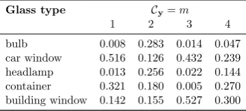
Table4 reports the values of p(Ty =t|Cy =m, D) computed usingp(Ty =

t) = 1/T and the hyperparameters αtm= 0.1 for all tand m.

Table4about here.

Incidentally, we remark that the choice of 0.1 as the value for the α’s did

not seem to matter much: we repeated five times the classification exercise

reported in Section5.2, setting theα’s to 0, 0.2, 0.3, 0.4 and 0.5, and in all

cases, the classifications given in Table 5 remained unchanged. Similarly,

the evidence evaluation error rates reported in Section6.1 were unaffected

by changing theα’s from 0.1 to 0.5.

As for the second term in (11), the posterior predictive distribution of y

conditional on its use type, configuration and the reference data, one has

p(y|Ty=t,Cy=m, D) =

= Z

p(y|Ty=t,Cy =m, ξm, D)p(ξm|Ty =t,Cy=m, D) dξm

= Z

p(y|Ty=t,Cy =m, ξm)p(ξm|Dm) dξm

= Eξm|Dm[p(y|Ty=t,Cy =m, ξm)], (16)

whereEξm|Dm denotes expectation with respect to the posterior distribution

of ξm. The density p(y|Ty = t,Cy = m, ξm) is provided by the Bayesian

hierarchical model (2) for elemental configuration m. To be more specific,

assuming that y is a vector consisting of ˜K measurements on each of ˜J

fragments from the same item of use typet and configuration m, then the

distribution ofy|Ty=t, ξm is given by formulae (3) and (4), after replacing

J with ˜J and K with ˜K:

Σt= (1_J˜_K˜1′J˜K˜)⊗Ω −1 t +

I_J˜⊗(1_K˜1′K˜)

⊗Ψ−1+I_J˜_K˜ ⊗Λ−1. (17)

Plugging (15) and (16) into (11) gives the expression for the use-type

prob-ability of a future itemy:

p(Ty=t|y, D) ∝ p(Ty=t)

αtm+Ntm

PM

r=1(αtr+Ntr)

Eξm|Dm[p(y|Ty =t,Cy=m, ξm)],

(18)

where the expectation on the right-hand side can be estimated by averaging

the densities p(y|Ty = t,Cy = m, ξm) over an MCMC sample from the

posterior ofξm, obtained as detailed in Section 4.1.

5.2 Classification results

A simulation study was conducted in order to assess the performance of the

composite model in classifying glass fragments into one of the five use types

(bulb, headlamp, container, car window or building window). Probabilities

that each set of fragments was from an item of a certain use type were

estimated using expression (18) with p(Ty = t) = 1/T and αtm = 0.1 for

all t and m. Fragments were classified into the use-type category with the

highest probability.

The simulation study used five-fold cross-validation with the reference data

D randomly divided into five parts, each consisting of 64 items. One part

was kept as test data consisting of unobserved glass itemsy. The remaining

four parts were considered as training data containing reference glass items

z, from which model parameters were estimated. This was repeated five

The classification results are shown in Table5, with Figure6giving an

indi-cation of the uncertainty about the classifiindi-cation of each item. The overall

misclassification rate was 20.6%, reflecting good classification performance

for bulbs, containers and headlamps, and poorer performance for car and

building windows. From Table 5, it is clear that misclassification of a

win-dow type is most often to the other winwin-dow type. This is because car and

building windows have a very similar elemental composition, thus making it

difficult to correctly distinguish between them based on this alone. Zadora

[1] reports improved classification rates for car and building windows when,

in addition to the elemental composition, the refractive index before and

after annealing is used.

Table5about here.

Comparing our classification results with those obtained using a

hierarchi-cal model that does not take into account the configurations, shows that

the composite model leads to a reduction in the number of items

misclas-sified (misclassification rates of 20.6% for the composite model compared

with 22.8% for the model without configurations). In addition, the

com-posite model achieves a lower misclassification rate (20.6%) than support

vector machines (SVM) [22] (22.8%). The composite model also

outper-forms SVM across two other classification performance measures: Cohen’s

kappa (κ = 0.721 for the composite model compared with 0.688 for SVM)

and Brier score (BS = 0.319 for the composite model, 0.447 for SVM).

Cohen’s kappa [23] is a measure of agreement ranging from 0 to 1 with

κ = 1 indicating perfect agreement. The Brier score [24] is a measure of

prediction strength with BS = 0 implying perfect predictions. For

without considering configurations areκ= 0.693 andBS = 0.338. In both

comparisons, the benefit of modelling the configurations is clear.

Figure6 about here.

6

Evidence evaluation

Glass fragments obtained from a suspect can be used as evidence in

sup-port of (or against) the proposition that the suspect was at the scene of the

crime. The statistical approach to evaluating the strength or value V of

such evidence stems from [25]; a recent overview is provided by [26, Chapter

10], whose terminology we adopt. Let E be the evidence, Hp the

prosecu-tion proposiprosecu-tion, Hd the defence proposition and I additional background

information related to the case. The value of the evidence for Hp, also

known in the forensic literature as thelikelihood ratio, is defined as the

fac-tor by which to multiply the prior odds on Hp, as a result of observing E:

V = Pr(E|Hp, I)/Pr(E|Hd, I). Typically, the probability statements in V

are obtained by integrating over the posterior distributions of unknown

pa-rameters, then the appropriate term isBayes factor [27] for Hp and against

Hd, on evidenceE.

More specifically, denote by x the measurements collected from a sample

of glass fragments found at the crime scene (source evidence) and by y

the measurements obtained from fragments found on the suspect (receptor

object), under the assumption that all fragments in y are from the same

item. The glass evidence comprises both control and recovered samples:

item as x, that is, the fragments found on the suspect originated from the

broken item found at the crime scene. The defence proposition,Hd, is that

yis not from the same item asx, that is, the fragments found on the suspect

originated from some source outwith the crime scene. The value of the glass

evidence is then

V = p(x,y|Hp, I) p(x,y|Hd, I)

. (19)

Here, we assume that two sets of fragmentsx and y do not come from the

same item if their elemental configurations do not match; that is, Cx6=Cy,

yielding V = 0. This assumption may not always hold in practice as it is

possible for two sets of fragments from the same item to have non-matching

configurations, although for the glass data, this occurs very rarely (less than

1% of the time). In the following, we assume that Cx =Cy =C =m. Let

Tx = t be the known use type of the glass recovered at the crime scene.

Under Hp, one has that Ty = Tx, while under Hd, the use type of y is

uncertain. Dropping in (19) the explicit conditioning on I, save for the

reference data setD used to assess the competing propositions, the known

elemental configurationC, and the known use type Tx of x, one has:

V = p(x,y|Tx=t,C=m, D, Hp)

p(x,y|Tx=t,C=m, D, Hd)

. (20)

We show in Appendix A.3thatV can be rewritten as

V = Eξm|Dm

p(x,y|T₍x,y)=t,C=m, ξm)

T

X

s=1

p(Ty =s|C=m, D)Eξm|Dm[p(x|Tx=t,C=m, ξm)p(y|Ty=s,C=m, ξm)]

,

(21)

wherep(Ty=s|C =m, D) is given in (15). The densityp(x,y|T(x,y)=t,C=

˜

J = ˜Jx+ ˜Jy is the total number of fragments obtained, ˜K is the number

of measurements taken on each fragment, and the covariance matrix Σthas

the expression given in (17). The densities p(x|Tx = t,C = m, ξm) and

p(y|Ty = s,C = m, ξm) in the denominator are of N_J˜

xKp˜ (1J˜xK˜ ⊗θt,Σtx)

and NJ˜yKp˜ (1J˜yK˜

⊗θt,Σty) respectively, where Σtx and Σty are given by

formula (17), with ˜J replaced by ˜Jx and ˜Jy.

6.1 Evidence evaluation results

The performance of the composite model in the evidence evaluation task was

assessed in terms of the percentage of false negative (FN) and false positive

(FP) answers produced in a simulation study. An FN occurs when glass

fragments from the same item are evaluated as originating from different

items, a decision that is made whenever V ≤ v, for some threshold value

v. An FP happens when glass fragments are from different items, but V >

v so that they are evaluated as coming from the same item. Here, V is

obtained using (21), with parameter values and resulting p(Ty = s|C =

m, D) estimates as in Table4.

Five-fold cross-validation was used in the simulation study to estimate the

percentages of FN and FP answers. Each test set consisted of 64 items with

the percentage of FN answers obtained by randomly choosing two fragments

from each item as the source evidence, x, and comparing them with the

remaining two fragments from the same item as the receptor sample,y. This

was repeated for each of the five test sets yielding a total of 320 same-source

comparisons. The percentage of FP answers was obtained by taking all 12

measurements from an item asxand all 12 measurements from another item

was repeated for each of the five test sets giving a total of 5× 64₂

= 10,080

comparisons. Note that because many more comparisons were made for

different-source pairs than for same-source pairs, estimates of FN rates are

more uncertain than those of FP rates.

Using as threshold v = 1, the rates of FNs and FPs produced by

cross-validation were 4.4% and 1.4%, respectively, which are improvements on

previous publications with similar glass databases; see [10]. However, the

two types of error are of different seriousness: because incorrectly evaluating

two sets of fragments as originating from the same item may contribute to

the conviction of an innocent person, emphasis should be placed on avoiding

false positives. This is readily achieved by varying the thresholdv. To each

value ofv there corresponds a pair of error rates and these are represented

in the receiver operating characteristic (ROC) curve displayed in Figure 7,

where as usual the true positive (TP) rate (TP rate = 1−FN rate) is plotted

against the FP rate. The ROC curve is very steep in the region of FP rates

close to 0: small reductions in the FP rate, say below 1%, can be achieved

only at the cost of noticeably increasing the FN rate to about 10% or more.

The value of the area under the curve is 0.99, a value of 1 is achieved by an

“ideal” procedure with zero FP rate and unit TP rate.

Figure7 about here.

7

Conclusion

We have presented a composite model to deal with a large point mass at

set was partitioned according to the presence or absence of the elements iron

and potassium, and a Bayesian hierarchical model was fit to each resulting

subset of the data. While this approach allows for the majority of

composi-tional zeros to be accounted for, a small proportion of zeros persists, as seen

from Figure3, mainly occurring when the element magnesium is absent from

a composition. To check whether accounting for these additional zeros would

improve results, we split configuration 2 in Table 2, (Fe,K), into two

con-figurations based on the presence or absence of magnesium, (Fe,K,Mg) and

(Fe,K,Mg). Repeating the analysis with the resulting five configurations

did not change or improve upon the classification and evidence evaluation

results obtained using the original four configurations.

Before proceeding with the analysis, we have applied a square root

transfor-mation to the ratios of chemical elements’ contents to that of oxygen. This

is a departure from the more commonly used ALR transformation. We have

found that, in addition to being more effective at stabilising the variability

in these data, use of the square root also meant that any remaining zeros in

the data did not require further special treatment such as replacement by a

small amount.

Our hierarchical model is more general than previous random effects models

for similar data [10,18] as it contains a fixed effect for use type of glass and

three levels of variability (item, fragment and measurement) and allows for

different variances for each use type of glass. A normality assumption was

made for the distribution of all random effects, which may not be ideal for

the between-item distribution in particular. An alternative would be to use

mixture models – this is an area of future work. However, the simplicity of a

satisfactory results, as is the case here in both classification and evidence

evaluation tasks.

The composite model outperforms SVM as well as a hierarchical model

with-out configurations in the classification task, with very good results obtained

for the classification of glass items of use types bulb, headlamp and

con-tainer. The relatively high overall misclassification rate of 20.6% is due to

the difficulty in distinguishing between car and building windows, which

are manufactured in a similar way and have similar elemental compositions.

However, whenever a window is misclassified, it is most often misclassified

as the other window type. Perhaps different glass measurements such as

the refractive index would be more useful in distinguishing between window

types.

The performance of the composite model in the evidence evaluation task is

also good. The FP and FN rates, obtained using cross-validation and giving

equal importance to the two types of error, were 1.4% and 4.4%, respectively.

More generally, the ROC curve (area under the curve = 0.99) shows that

very low FP rates can be achieved, if one is willing to accept moderate FN

rates.

Acknowledgements

The authors would like to thank Prof. Grzegorz Zadora for providing us with

access to the glass database used in the analysis. Gary Napier acknowledges

financial support under a doctoral training grant from the U.K. Engineering

A

Appendix

A.1 Full conditional distributions

The full conditional distribution of all the unknown quantities in the model

are reported below. We use “| · · ·” to mean “conditionally on all the other

variables”.

• θt| · · · ∼Np( ˜φt,Φ˜−t1), θt>0,

where ˜φ_t= ˜Φ−_t1hJKIt(¯zt···−¯bt·−¯ct··)

i

, and ˜Φt=JKItΛ + Φ.

• bti| · · · ∼Np( ˜ωti,Ω˜−t1),

where ˜ωti = ˜Ω−t1

h

JKΛ(¯zti··−θt−¯cti·)

i

, and ˜Ωt=JKΛ + Ωt.

• ctij | · · · ∼Np( ˜ψtij,Ψ˜−1),

where ˜ψ_tij = ˜Ψ−1hKΛ ¯ztij·−θt−bti

i

, and ˜Ψ =KΛ + Ψ.

• Ωt| · · · ∼Wp( ˜d1t,A˜t),

where ˜d1t=d1t+It, and ˜At=At+PI_i=1t btib′ti.

• Ψ| · · · ∼Wp( ˜d2,B˜),

where ˜d2 =d2+JPTt=1It, and ˜B =B+PTt=1 PIt

i=1 PJ

j=1ctijc′tij. • Λ| · · · ∼Wp( ˜d3,C˜),

where ˜d3=d3+JKPTt=1It, and ˜C=C+PTt=1 PIt

i=1 PJ

j=1 PK

k=1(ztijk−

A.2 MH move on θ and b jointly

This move updates simultaneously the fixed effectθtand the random effects

at item levelbti, separately for each use typet. The candidate state is chosen

to leaveθt+btiunchanged, so that it shares with the current state the same

value of the likelihood. The candidate for the fixed effect is obtained as

˜

θt=θt+v,

where v = (v1, . . . , vp)′, with components vl ∼ U nif(−δtl, δtl)

indepen-dently, with interval widths determined from a preliminary run. The

candi-dates for the random effects are then set to

˜

bti =bti−v, i= 1, . . . , It.

Since the likelihood is left unchanged, the ratio of target densities reduces

to the ratio of prior densities evaluated at the candidate and current state.

Then, following the approach in§2.2 of [20], the acceptance probability can

be computed as

α= min

1,p(˜θt)p(˜bt|Ωt) p(θt)p(bt|Ωt)

˜ f(˜v) f(v)

∂(˜θt,b˜t,˜v)

∂(θt,bt,v)

wheref is the density, uniform on a p-hyperrectangle, of the random

reverse move. The absolute value of the determinant of Jacobian matrix is

∂(˜θt,˜bt,v)˜

∂(θt,bt,v)

=

Ip 0p,pIt Ip

0pIt,p IpIt −1It ⊗Ip

0p,p 0p,pIt −Ip

= 1.

Therefore the acceptance probability only involves the prior density at the

current and candidate values:

α= min

1,p(˜θt)p(˜bt|Ωt) p(θt)p(bt|Ωt)

.

A.3 Computing the evidence value V

Here we show how to derive the expression (21) for V. Starting with (20),

V = p(x,y|Tx=t,C=m, D, Hp)

p(x,y|Tx=t,C=m, D, Hd)

= R

p(x,y|Tx=t,C=m, ξm, D, Hp)p(ξm|Tx=t,C=m, D, Hp) dξm

R

p(x,y|Tx=t,C=m, ξm, D, Hd)p(ξm|Tx=t,C=m, D, Hd) dξm

.

(22)

For the first term of the integrand in the numerator one has

p(x,y|Tx=t,C=m, ξm, D, Hp) = T

X

s=1

p(x,y|Tx=t,Ty =s,C=m, ξm, D, Hp)

·p(Ty=s|Tx=t,C=m, ξm, D, Hp)

= p(x,y|Tx=t,Ty=t,C=m, ξm, D)

since Hp implies that Ty = Tx = t, the known use type of x, and we use

the notationT_(x,y) to emphasize that, underHp,xandyare measurements

from the same glass item. Then the numerator of (22) can be written as

Z

p(x,y|T(x,y)=t,C =m, ξm)p(ξm|Dm) dξm=

Eξm|Dm

p(x,y|T₍x,y)=t,C=m, ξm)

. (23)

Consider next the denominator of (22). Under Hd and conditional on the

parametersξm,xis independent of yso that

p(x,y|Tx=t,C=m, ξm, D, Hd) =

= p(x|Tx=t,C =m, ξm, D, Hd)p(y|Tx=t,C=m, ξm, D, Hd)

= p(x|Tx=t,C =m, ξm)p(y|C=m, ξm, D). (24)

The second term on the right hand side of (24) can be written as

p(y|C=m, ξm, D) = T

X

s=1

p(y|Ty=s,C=m, ξm, D)p(Ty=s|C=m, ξm, D)

=

T

X

s=1

p(y|Ty=s,C=m, ξm)p(Ty =s|C =m, D),

wherep(Ty=s|C =m, D) is given in (15). It then follows that the

denom-inator of (22) is

Z

p(x|Tx=t,C=m, ξm)

" _T X

s=1

p(y|Ty =s,C=m, ξm)p(Ty=s|C=m, D)

#

p(ξm|Dm) dξm=

=

T

X

s=1

p(Ty=s|C =m, D)

References

1. Zadora G. Classification of glass fragments based on elemental

compo-sition and refractive index. J. Forensic Sci.2009; 54(1):49–59.

2. Aitchison J. The statistical analysis of compositional data. Chapman &

Hall, 1986.

3. Rayens WS, Srinivasan C. Box-Cox transformations in the analysis of

compositional data. J. Chemometr.1991; 5(3):227–239.

4. Egozcue JJ, Pawlowsky-Glahn V, Mateu-Figueras G, Barcel´o-Vidal C.

Isometric logratio transformations for compositional data analysis.

Math. Geol.2003; 35(3):279–300.

5. Scealy JL, Welsh AH. Regression for compositional data by using

dis-tributions defined on the hypersphere. J. R. Stat. Soc. B 2011; 73(3):

351–375.

6. Scealy JL, Welsh AH. Fitting Kent models to compositional data with

small concentration. Stat. Comput. 2014; 24(2): 165–179.

7. Wang H, Liu Q, Mok HMK, Fu L, Tse WM. A hyperspherical

trans-formation forecasting model for compositional data. Eur. J. Oper. Res.

2007; 179(2):459–468.

8. Campbell GP, Curran JM, Miskelly GM, Coulson S, Yaxley GM,

Grun-sky EC, Cox SC. Compositional data analysis for elemental data in

forensic science. Forensic Sci. Int. 2009; 188(1–3):81–90.

9. Stewart C, Field C. Managing the essential zeros in quantitative fatty

10. Neocleous T, Aitken CGG, Zadora G. Transformations for

composi-tional data with zeros with an application to forensic evidence

evalua-tion. Chemometr. Intell. Lab. 2011; 109(1):77–85.

11. Box GEP, Cox DR. An analysis of transformations. J. R. Stat. Soc. B

1964; 26(2):211–252.

12. Mart´ın-Fern´andez JA, Barcel´o-Vidal C, Pawlowsky-Glahn V. Dealing

with zeros and missing values in compositional data sets using

nonpara-metric imputation. Math. Geol.2003; 35(3):253–277.

13. Mart´ın-Fern´andez JA, Barcel´o-Vidal C, Pawlowsky-Glahn V. Zero

re-placement in compositional data sets. In Kiers H, Rasson J, Groenen P,

Shader M, editors,Proceedings of the 7th Conference of the International

Federation of Classification Societies, (University of Namur (Belgium)),

pages 155–160. Springer-Verlag, Berlin, 2000.

14. Palarea-Albaladejo J, Mart´ın-Fern´andez JA, G´omez-Garc´ıa JG. A

para-metric approach for dealing with compositional rounded zeros. Math.

Geol.2007; 39(7):625–645.

15. Butler A, Glasbey C. A latent Gaussian model for compositional data

with zeros. J. R. Stat. Soc. C 2008; 57(5):505–520.

16. Leininger TL, Gelfand AE, Allen JM, Silander Jr JA. Spatial regression

modeling for compositional data with many zeros. J. Agr. Bio. Envir.

St.2013; 18(3):314–334.

17. Trejos T, Almirall JR. Sampling strategies for the analysis of glass

fragments by LA-ICP-MS Part 1: micro-homogeneity study of glass

18. Aitken CGG, Lucy D. Evaluation of trace evidence in the form of

mul-tivariate data. J. R. Stat. Soc. C 2004; 53(1):109–122.

19. Casella G, George EI. Explaining the Gibbs Sampler. Am. Stat.1992;

46(3):167–174.

20. Green PJ. Trans-dimensional Markov chain Monte Carlo. In Green PJ,

Hjort NL, Richardson S, editors, Highly structured stochastic systems,

pages 179–196. Oxford: Oxford University Press, 2003.

21. R Development Core Team. R: A language and environment for

sta-tistical computing. R Foundation for Stasta-tistical Computing, Vienna,

Austria, 2011. URL http://www.R-project.org.

22. Cortes C, Vapnik VN. Support-vector networks. Mach. Learn.1995; 20

(3):273–297.

23. Cohen J. A coefficient of agreement for nominal scales. Educ. Psychol.

Meas. 1960; 20(1):37–46.

24. Brier GW. Verification of forecasts expressed in terms of probability.

Mon. Weather Rev.1950; 78(1):1–3.

25. Lindley DV. A problem in forensic science. Biometrika 1977; 64(2):

207–213.

26. Aitken CGG, Taroni F. Statistics and the evaluation of evidence for

forensic scientists. John Wiley and Sons, 2004.

27. Kass RE, Raftery AE. Bayes factors.J. Am. Statist. Ass.1995; 90(430):

Table 1: Frequency of zero measurements by chemical element.

Element O Si Na Ca Al Mg K Fe

Frequency 0 0 0 108 205 265 1168 3036

Table 2: Presence (Fe, K) and absence (Fe,K) at item level by use type.

Glass type Configurationm Total

1: Fe, K 2: Fe, K 3: Fe, K 4: Fe, K

bulb 0 25 0 1 26

car window 23 40 11 20 94

headlamp 0 14 0 2 16

container 12 48 0 19 79

building window 7 55 15 28 105

Table 3: Standard deviations (multiplied by 10) from covariance matrices Ω−1

t ,

Ψ−1 _{and Λ}−1_{. For Ω}−1

t , t= 1, . . . ,5 correspond to use types: bulb, car

window, headlamp, container and building window.

Na Mg Al Si K Ca

Ω−₁1 0.95 0.94 0.28 0.65 1.12 1.34

Ω−₂1 0.10 0.25 0.26 0.30 0.15 0.26

Ω−₃1 0.18 0.91 0.52 0.51 0.31 0.78

Ω−₄1 0.12 0.51 0.15 0.44 0.19 0.37

Ω−₅1 0.10 0.13 0.13 0.26 0.13 0.22

Ψ−1 0.07 0.05 0.09 0.30 0.11 0.25

Table 4: Use type probabilities p(Ty =t|Cy =m, D), with αtm = 0.1 for all t

andmandp(Ty=t) = 1/T.

Glass type Cy=m

1 2 3 4

bulb 0.008 0.283 0.014 0.047

car window 0.516 0.126 0.432 0.239

headlamp 0.013 0.256 0.022 0.144

container 0.321 0.180 0.005 0.270

Table 5: Classification of each glass item into one of five use type categories.

Classification Glass type

bulb car window headlamp container building window Total

bulb 25 0 1 0 1 27

car window 1 74 0 4 29 108

headlamp 0 1 15 1 1 18

container 0 2 0 72 6 80

building window 0 17 0 2 68 87

Total 26 94 16 79 105 320

Mean

Standard de

viation

−8 −6 −4 −2 0

0.0

0.5

1.0

1.5

2.0

2.5

3.0

Mean

0.0 0.2 0.4 0.6 0.8 1.0

0.00

0.02

0.04

0.06

0.08

0.10

Figure 1: Plots of fragments’ standard deviations against corresponding means,

using the ALR (left panel) and the square root (right panel) transforma-tions. For the ALR, 0.005 was added to all compositional zeros. Seven pairs (mean, sd) are plotted for each fragment, one for each element of

0.30

0.40

0.50

Na

0.00

0.10

0.20

Mg

0.00

0.10

0.20

Al

0.65

0.80

Si

0.00

0.15

0.30

K

0.0 0.2 0.4

0.00

0.06

0.12

Ca

F

e

0.30 0.40 0.50

Na

0.00 0.10 0.20

Mg

Bulb Car window Headlamp Container Building window

0.00 0.10 0.20

Al

0.65 0.75 0.85

Si

0.00 0.15 0.30

K

Figure 2: Scatterplots of all item means from the database. The mean of each

0.30

0.40

0.50

Na

0.00

0.10

0.20

Mg

0.00

0.10

0.20

Al

0.65

0.75

0.85

Si

0.0 0.1 0.2 0.3 0.4

0.00

0.10

0.20

0.30

Ca

K

0.30 0.40 0.50

Na

0.00 0.10 0.20

Mg

Bulb Car window Headlamp Container Building window

0.00 0.10 0.20

Al

0.65 0.75 0.85

Si

Figure 3: Scatterplots of the item means for items with configuration 2 from Table

0.32 0.38 0.44 θ₁ 0.442 0.448 θ₂ 0.425 0.445 θ₃ 0.430 0.438 θ₄ θ₅ Na 0.432 0.438

0.04 0.10 0.16 0.200 0.215

0.00 0.10 0.10 0.12 0.14

Mg 0.208 0.214 0.130 0.150 0.085 0.100 0.08 0.14 0.120 0.130 Al 0.080 0.088

0.74 0.78 0.82 0.83 0.85

0.80 0.86 0.79 0.81 0.83

Si

0.805 0.825

0.15 0.25 0.060 0.070

0.14 0.17 0.20 0.075 0.090

K

0.050 0.056

0.05 0.15 0.340 0.355

0.32

0.36

0.40

0.44

Na

0.00

0.10

0.20

Mg

0.08

0.12

0.16

Al

0.75

0.80

0.85

Si

0.05 0.15 0.25 0.35

0.05

0.15

0.25

Ca

K

0.32 0.36 0.40 0.44

Na

0.00 0.10 0.20

Mg

Bulb Car window Headlamp Container Building window

0.08 0.12 0.16

Al

0.75 0.80 0.85

Si

Figure 5: Scatterplots of the draws from the posterior distribution of θt in the

Bulb (1) 1 2 3 4 5

Car window (2)

1 2 3 4 5 Headlamp (3) 1 2 3 4 5 Container (4) 1 2 3 4 5

Building window (5)

1 2 3 4 5 Bulb (1) Car window (2) Headlamp (3) Container (4) Building window (5)

Figure 6: Plot of the classification probabilities in five-fold cross validation. Each

0.0 0.2 0.4 0.6 0.8 1.0

0.0

0.2

0.4

0.6

0.8

1.0

False positive rate

T

rue positiv

e r

ate

AUC = 0.99