This is a repository copy of Public Investment and Re-election Prospects in Developed Countries.
White Rose Research Online URL for this paper: http://eprints.whiterose.ac.uk/82784/
Version: Accepted Version
Article:
Katsimi, M. and Sarantides, V. (2015) Public Investment and Re-election Prospects in Developed Countries. Southern Economic Journal, 82 (2). pp. 471-500. ISSN 0038-4038 https://doi.org/10.4284/0038-4038-2013.181
This is the peer reviewed version of the following article: Katsimi, M. and Sarantides, V. (2015), Public investment and reelection prospects in developed countries. Southern Economic Journal, 82: 471–500. doi: 10.4284/0038-4038-2013.181, which has been published in final form at http://dx.doi.org/10.4284/0038-4038-2013.181. This article may be used for non-commercial purposes in accordance with Wiley Terms and Conditions for Self-Archiving (http://olabout.wiley.com/WileyCDA/Section/id-820227.html).
eprints@whiterose.ac.uk https://eprints.whiterose.ac.uk/ Reuse
Unless indicated otherwise, fulltext items are protected by copyright with all rights reserved. The copyright exception in section 29 of the Copyright, Designs and Patents Act 1988 allows the making of a single copy solely for the purpose of non-commercial research or private study within the limits of fair dealing. The publisher or other rights-holder may allow further reproduction and re-use of this version - refer to the White Rose Research Online record for this item. Where records identify the publisher as the copyright holder, users can verify any specific terms of use on the publisher’s website.
Takedown
If you consider content in White Rose Research Online to be in breach of UK law, please notify us by
Public Investment and Re-election Prospects in Developed Countries
Margarita Katsimia and Vassilis Sarantidesb
August 2014
Abstract
A growing body of literature suggests that office-motivated politicians manipulate fiscal policy instruments in order to enhance their re-election prospects. This paper directly
examines the impact of fiscal policy on incumbents’ re-election prospects by focusing on the impact of public investment. This impact is estimated using a panel of 20 OECD countries over the period 1972-1999. We find that the level of public investment in the earlier years of an incumbent's term in office improves their re-election prospects, whereas election year manipulation of public investment is neither rewarded nor punished. Our evidence also suggests that, after controlling for the level of deficit and public investment, the level of government revenue both in the election and non-election years does not seem to affect re-election prospects. Moreover, we find that deficit creation during re-elections and in non-election years are not rewarded by voters.
JEL Classification: D72, E62
Keywords: Political budget cycles, elections, quality of public expenditure, public investment
Acknowledgements: Without implicating, we wish to thank David Cuberes, Andy Dickerson, Georgios Efthyvoulou, Paul Mosley, Niklas Potrafke, Simon Schnyder, Grigorios Siourounis and participants in seminars at the Athens University of Economics and Business, at Birkbeck College, University of London in the 2011 European Public Choice Society conference and in the 2011 Annual Meeting of the Association of Southern European Economic Theorists. We also want to thank the co-editor, and two anonymous referees for many helpful comments and suggestions which led to substantial improvements in the paper. The usual disclaimer applies.
a
Corresponding author. Athens University of Economics and Business and CESifo. Address: AUEB, Department of International and European Economic Studies, Patision Str 76, Athens 10434, Greece. Tel: 210-8203179, Fax: ++30-210-8214122. E-mail address: mkatsimi@aueb.gr
b
1. Introduction
Since the seminal work of Nordhaus (1975), a rich body of literature suggests that
office-motivated incumbents manipulate fiscal policy in order to improve their chances to get
re-elected.1 In a rational expectations framework, political budget cycles (PBC) still arise under
the driving assumption of temporary information asymmetries between voters and politicians
regarding the competence level of the latter.2 Electoral manipulation of fiscal policy can also
affect the composition rather than the level of public spending. Rogoff (1990) provided a firm
theoretical foundation showing that electorally motivated incumbents signal their competence
by shifting public spending toward more visible government consumption and away from
public investment goods that are mostly long-term projects and will increase voters’ utility
upon completion.
Many empirical studies find evidence of electorally timed shifts in the composition of
public spending not only at the national but also at the local level. It is important to note,
though, that for studies conducted at the local level, evidence suggests that authorities attempt
to signal their competence by expanding the level of investment spending (see, e.g., Khemani
(2004); Drazen and Eslava (2010)) while policymakers at the national level provide
immediate benefit to voters through consumption or taxation whereas capital spending
decreases (see, e.g., Vergne (2009); Katsimi and Sarantides (2012)). These findings may
reflect that Rogoff’s (1990) assumption of lower visibility of capital expenditures (e.g.,
infrastructure) conforms much better to central government rather than to local level
spending.
In fact, manipulation of the composition of fiscal policy seems particularly relevant in
developed economies in which the incumbent may avoid deficit creation due to the fear of
voters’ disfavour. Indeed, Brender and Drazen (2013) find that election years are associated
with larger expenditure composition changes in established democracies, the majority of
which are developed economies, while incumbents in ‘new democracies’ tend to increase the
overall level of expenditures in election years (see Brender and Drazen (2005)).
1 In contrast, the partisan approach focuses on the role of government ideology on fiscal policy priorities (see, e.g., Hibbs
(1977); Alesina (1987); Chappell and Keech (1988)). For empirical evaluations of the impact of ideology on the composition of fiscal policy, see, among others, Potrafke (2011).
2
For a discussion of the implications of theoretical PBC adverse selection and moral hazard type models, see Shi and Svensson (2003). Empirical evidence on the budgetary impact of elections, until recently, suggested that PBC was a phenomenon of less-developed countries (see, e.g., Schuknecht (1996); Shi and Svensson (2006)) or of the so-called ‘new
A complementary literature investigates the impact of fiscal policy choices on the
voting behaviour and on incumbents’ re-election prospects. Empirical studies that attempt to assess the impact of fiscal policy on re-election prospects either include fiscal variables in the
estimation of a voting function or they employ binary models in order to estimate the
probability of an incumbent's re-election.
The first approach belongs to the literature on economic voting based on the seminal
papers of Goodhart and Bhansali (1970), Mueller (1970) and Kramer (1971). This literature
estimates popularity/voting functions in order to investigate the impact of economic variables
on voting behaviour. Based on the “Responsibility Hypothesis" according to which voters
hold the government responsible for the economy, an extensive literature investigates the
channels through which voting behaviour depends on voters' economic experiences and on
their perception and evaluation of the macro economy. However, most multi-country studies
that estimate the impact of the economy on the incumbents’ share of the votes at national
elections measure economic performance in terms of output growth, inflation and
unemployment without taking into account government's fiscal performance (for a survey see
Paldam (1981); Norpoth et al. (1991); Nannestad and Paldam (1994); Lewis-Beck and
Paldam (2000)). An exception is Veiga (2013) who finds that voters reward positive budget
balances whereas after the 2008 crisis there is evidence that they have become more
determinedly fiscally conservative.
The second approach of estimating a binary model has been used by the majority of
the limited number of empirical studies on the impact of fiscal policy on the incumbent’s re
-election prospects at national level.3 Their findings suggest that in established democracies,
well-informed voters act as fiscal conservatives and punish rather than reward loose fiscal
policies at the polls (see, e.g., Brender and Drazen (2008) and Alesina et al. (2012)).4
For elections at the state and local levels researchers have estimated both binary
models and voting functions. The dominant result that voters penalize expansive fiscal
policies (see, among others, Peltzman (1992); Brender (2003)) has recently been challenged
for some developing countries (see, e.g., Akhmedov and Zhuravskaya (2004); Sakurai and
Menezes-Filho (2008); Jones et al. (2012)). Regarding the relationship between public
investment expenditures and re-election prospects, limited studies using both approaches are
3
Although they do not directly test the impact of fiscal policy on re-election, Klomp and de Haan (2013) find that election-motivated budget cycles have a significant positive (but fairly small) effect on the electoral support for the political parties in government.
4 It should be noted that, under certain assumptions regarding preferences and the nature of uncertainty, a number of
exclusively concentrated at the local level and their results are mixed (see, e.g., Veiga and
Veiga (2007) and Drazen and Eslava (2010)).
Two points should be noted about these contradicting results at the local level. First,
as emphasized by Brender and Drazen (2008), empirical conclusions drawn from country
studies should, strictly speaking, be limited to these countries. Given that fiscal items that are
clearly identifiable as provincial government responsibilities differ from one country to
another, it is difficult to derive more general policy conclusions from country studies.
Secondly, as already mentioned, local authorities tend to expand expenditures on investment
projects near elections, indicating that Rogoff’s (1990) prediction of shifts in public spending
toward more visible government consumption and away from public investment goods may
not hold for local governments in which public investment may not be characterized by low
visibility.
The contribution of the present paper is found in its focus on the role of national
public investment as an instrument for affecting re-election prospects of the incumbent in
developed countries. We believe that this is an important step because we empirically test the
following predictions implicitly derived from the existing literature: Firstly, if public capital
spending is invisible, as suggested by Rogoff (1990), then the manipulation of public
investment just before elections should not affect the re-election prospects of the incumbent.
We analyze the impact of public investment on voting behaviour and re-election probability
by using a sample of established democracies, because we believe it makes sense to look at
the countries in which this type of electoral manipulation has been supported by empirical
evidence (see Katsimi and Sarantides (2012) and Brender and Drazen (2013)). Our paper
complements this literature by testing whether electoral manipulation in the form of a fall in
public investment in developed established democracies found by Katsimi and Sarantides
(2012) affects the incumbents’ re-election prospects.5 Secondly, public investment
expenditures that occurred in the earlier years of an incumbent’s term in office should be
observable by voters near the completion of the term, since these expenditures are mostly
long-term projects which are noticed with a lag. Given the positive impact of productive
expenditure on long-run growth emphasized by the relevant literature, we expect voters to
5
reward a rise in this type of expenditure.6 For a given level of deficit, voters are likely to
reward this type of expenditure if they perceive it as more 'productive' than current
expenditure.
We test the impact of public investment on re-election prospects by estimating both a
binary model and a voting function. Our empirical results using a sample of 20 OECD
countries over the period of 1972-1999 suggest that the level of public investment in the
earlier years of an incumbent's term in office improves re-election prospects whereas election
year manipulation of public investment is neither rewarded nor punished.7 Given that public
investment expenditures at the national level are mostly long-term projects, this result is
consistent with Rogoff’s (1990) assumption of the lower visibility of this type of expenditure and explains previous empirical findings for electoral manipulation of public investment.
Our paper builds on the existing literature on the effect of fiscal policy on electoral
results at the national level. Brender and Drazen (2008) study a sample of 77 countries over
the period 1960-2003 and find that deficits in an election year are punished by voters in
developed countries that are established democracies. Alesina et al. (2012) analyse a sample
of 19 OECD countries for the 1975-2008 period and find no evidence that fiscal adjustments
increase the turnover of governments. Veiga (2013) uses a voting function for a panel of 15
European Union countries for the 1970-2011 period in order to analyze the impact of the
European integration process on voters’ evaluations of governments’ economic performance
and finds that the vote share of the government depends positively on budget surpluses.
However, although our paper also examines the impact of deficit creation on
re-election prospects, its main focus on the impact of public investment and the composition of
public spending is novel. Moreover, it investigates whether the main predictions of the
existing literature regarding the political cost of electoral deficit creation can be found after
controlling for other elements of the government's budget constraint such as revenue and
expenditure composition. We find that, similar to Brender and Drazen (2008), deficit creation
both in the election year and during the term in office is never rewarded by voters in
developed countries (it is either punished or it does not affect the re-election prospects). We
also find some evidence that the vote share of the main government party increases with the
level of budget surplus in the election period which is a result consistent with the findings of
Veiga (2013). Our results are not directly comparable to Alesina et al. (2012) who use a
6 Paul et al. (2004) and Henderson and Kumbhakar (2006) emphasize the positive impact of public capital on productivity
whereas Kneller et al. (1999) and Bleaney et al. (2001) find a positive effect of productive expenditures on long-run growth.
7
different specification and focus mainly on large fiscal adjustments but their finding that
fiscal adjustments are not punished by voters is consistent with our results.
The remainder of the paper is organized as follows. Section 2 describes the data,
specifies the econometric model, and contains our basic findings. Section 3 reports the results
of robustness tests. In section 4 we test whether our results are replicated by estimating a
voting function. The last section concludes.
2. Empirical Analysis
2.1. Data and estimation method
In order to estimate the effect of public investment expenditure and the composition of public
expenditure on re-election prospects, we use data for 20 OECD countries over the period of
1972-1999.8 Our sample consists of countries that can be characterised as developed
economies and established democracies, since the existing literature indicates that
manipulation of the composition of fiscal policy seems particularly relevant in countries with
these characteristics.9 The countries in our sample are also included in the sample used by
Brender and Drazen (2008), Katsimi and Sarantides (2012) and Brender and Drazen (2013)
allowing us to relate our results with the findings of these papers. In line with Brender and
Drazen (2008), we estimate the impact of fiscal policy on the incumbent's probability of
re-election in a binary model although in a later section we test the robustness of our results by
estimating a voting function. The dependent variable re-election is based on information from
the World Statesmen Encyclopedia and from the Inter-Parliamentary Union database. These
data allow us to follow the terms of individual leaders and parties in office from appointment
to termination and to associate them with election dates. It is worth noting that we only
include legislative elections for countries with parliamentary political systems and
presidential elections for countries with presidential systems. In line with Brender and Drazen
(2008), the re-election variable includes observations in which the leader (the president for
the United States and the prime minister for all other countries of our sample) has been in
8
A key variable for our empirical analysis is not available after 1999, as discussed in the following.
9
office for at least two years prior to the elections. It takes value 1 if the incumbent chief
executive is re-elected and 0 otherwise. It also allows for the following special cases:
(i) In cases in which the leader quits within the year of the election, re-election receives
the value 0.
(ii) In cases in which, during the election year, a leader is replaced because she/he died or
resigned due to health problems, election takes the value 1 if the successor leader gets
re-elected and 0 otherwise.
(iii) For the United States, where the president is subject to a legal limit, re-election
receives the value 1 if the reigning leader’s party wins the election and 0 if it loses.10
(iv) Finally, in a coalition government, the re-election variable takes the value 1 if the
appointed prime minister comes from the same party as that of the prime minister before the
elections, and 0 otherwise. In addition, to ensure that the prime minister has not been changed
because he became unpopular, we consider re-election only in the case in which the party of
the appointed prime minister of the governing coalition received in the current elections a
higher vote share in comparison to the previous elections. Overall we have 106 campaigns in
which the leader was re-elected in 58 cases.11
Regarding our main variables of interest, we obtain our fiscal data from the ‘Global
Development Network Growth Database’ (GDNGD), whose primary source is the IMF
"Government Finance Statistics" (GFS) database. It should be noted that GFS is the only
multi-country data source for disaggregated central government data. For this reason, it is the
standard database used in empirical research studying either aggregate fiscal variables (see,
e.g., Brender and Drazen (2008)) or the composition of fiscal policy instruments (see
Schuknecht (2000); Vergne (2009)).12
Unfortunately, we cannot expand our dataset beyond the 1972-1999 period since GFS
modified the methodology of calculating the fiscal variables. In fact GFS until the late
nineties has been calculated using Government Finance Statistics Manual 1986 (GFSM
10
In our sample, in the US elections of 1988, the candidate could not run for re-election after the termination of the second mandate. Besley and Case (1995) show that the candidate who cannot run for re-election behaves differently regarding the manipulation of public expenditures. In contrast, though, it can be said that some party loyalty can justify the maintenance of public budget manipulation. To confirm that the results are robust, when we drop this observation our results remain unaffected.
11
Although we follow the leader’s re-election, in order to lengthen our sample, we follow the party’s re-election for special cases (ii), (iii), and (iv). However, when we narrow the sample in order to follow leader's re-election in all cases, our results remain unaffected.
12 We use central government data for several important reasons: Firstly given that general government data include all
1986) classification, while data beyond this point have been calculated according to the
Government Finance Statistics Manual 2001 (GFSM 2001). The new GFSM 2001
classification provides observations for the years 1990-2011, but not for our main variable of
interest, namely public investment expenditures. This means that we can neither estimate our
equations for two separate samples (1972-1999) and (1990-2011), nor harmonize the data
streams for both classifications and re-run regressions from 1972 to 2011.
We analyze the impact of public investment on re-election prospects, by estimating two
different specifications:
In the first one we are interested in the impact of the overall capital spending of the
incumbent during her term in office. Therefore, we include on the right hand side of our
specification a variable capital term defined as the average of capital expenditures during the
leader’s current term in office, scaled by GDP and expressed as percentage. Likewise, in order to investigate the impact of composition of expenditures on re-election prospects, we
construct a variable composition term defined as the percentage of capital to current
expenditures during the term in office of the incumbent.13 Both variables cover the whole
period of leader’s current term in the office, starting with the year after the previous election
and including the election year of current elections.14
In the second specification we investigate the central question of our paper, which is
whether the pre-electoral deviation of capital expenditures affects re-election prospects (see
also Veiga and Veiga (2007); Sakurai and Menezes-Filho (2008)). Similar to the first
specification, we are interested in public investment as well as the composition of public
spending. Regarding public investment, we split the variable capital term into capital
deviation and capital non-election. The former reflects the change in capital/GDP percentage
in the election year relative to the average of the previous years since the last election. The
latter is the average of capital/GDP percentage starting with the year after the previous
election and excluding the election year of current elections. Moreover, in direct analogy to
the first specification, we focus on the ratio of capital/current spending and we split
composition term into composition deviation and composition non-election.
Following Kneller et al. (1999) and Drazen and Eslava (2010), our empirical method is
based on a full specification of the government budget constraint. Kneller et al. (1999, pp
174-5) show that incomplete specification of the budget constraint results in substantial
13
According to the descriptive statistics in the Appendix A, the average of our sample for the variable composition term is 8.183. This means that capital spending is on average 8.183% of the current expenditure.
14
biases in parameter estimates.To address this problem, we want to include in our empirical
analysis all elements of the budget constraint but one in order to avoid perfect
multi-collinearity. Therefore we add in our specification the following fiscal variables: i) the central
government’s budget surplus/deficit, which according to Brender and Drazen (2008) is
positively/negatively related to re-election prospects in developed economies and ii) the
central government’s total revenues.15
In accordance to the definition of variables capital and
composition, we construct for central government’s budget surplus/deficit the variables
surplus term, surplus deviation and surplus non-election. Similarly for total revenues we
construct the variables revenues term, revenues deviation, and revenues non-election. Fiscal
variables surplus and revenues are scaled to GDP and expressed as percentages.
Apart from the fiscal variables, we include in our estimations the following political and
socio-economic control variables that we expect to affect re-election prospects:
(i) Macroeconomic conditions: We control for a number of macroeconomic variables
that, according to the relevant literature, are expected to affect voting behaviour (see, e.g.,
Peltzman (1992); Alesina and Rosenthal (1995), Brender and Drazen (2008); Aidt et al.
(2011) and Alesina et al. (2012)). These are the average growth rate of output (growth term),
the average inflation rate (inflation term), and the average unemployment rate (unemployment
term) during the term in office. Our data for growth term and inflation term are taken from
the World Bank's World Development Indicators, while those for unemployment term are
from the OECD Labour Force Statistics.16
(ii) New democracy effect: Based on the approach of Brender and Drazen (2005), we
consider as elections held in a ‘new democracy’ the first four elections after a shift to a
democratic regime, indicated by the first year of a string of uninterrupted positive polity
values as obtained from the POLITY IV annual time series. We expect that in 'new
democracies', the first period after the transition to a democratic regime may be characterized
by underdeveloped democratic institutions that may lead to an incumbency advantage (e.g.,
limited media independence).17
15
In order to avoid perfect multi-collinearity, we omit current expenditures from our specification but our results remain the same if we omit revenues instead. Regarding the interpretation of the results, the estimated coefficient on the fiscal variable measures the marginal impact of this variable on re-election prospects, net of the marginal impact of the fiscal variable that we exclude from the specification and is assumed to be the financing element. This implies that current expenditures are the financing element in columns (1) and (2) and total expenditures in columns (3) and (4).
16 It is worth noting that the macroeconomic variables do not seem to display problematic correlations. In addition, when the
variable growth term, which does not affect re-election prospects, is dropped from the specification, the results remain unaffected.
17
(iii) Level of “voter awareness”: A large body of theoretical literature agrees that
electoral accountability depends positively on the level and the quality of the information
available to voters (Persson and Tabellini (2000); Besley and Prat (2006); Pande (2011)).
Several recent empirical studies use the educational background of the population as a proxy
for “voter awareness”, meaning the ability of electorate to process available information that comes with education (see, among others, Akhmedov and Zhuravskaya (2004); Aidt et al.
(2011)). We expect that this ability may have an impact on voters’ evaluation of
government's policies thereby affecting the incumbent's re-election prospects. We proxy
“voter awareness” with the illiteracy rate among the population aged 15 years old and above obtained by Barro and Lee (2010).
(iv) Cabinet characteristics: In order to check whether cabinet ideology actually matters
for re-election, we create the dummy variable left (right) that receives the value 1 if the share
of seats in the cabinet for left (right) wing parties is larger than 66.6 percent. Moreover, we
create the dummy variable centre that takes the value 1 if the share of seats in the cabinet for
centrist parties is higher than 50%, or if we have right-centre or left-centre complexion where
the centre party holds more than 33.3 percent of the seats. Additionally, we create the dummy
variable fragmentation that takes the value 1 when left and right parties form a government
that is not dominated by one side or the other.18 Finally, we create the dummy variable
coalition that takes the value of 1 if the cabinet includes ministers from more than one party
and 0 otherwise. Data for the type of government and on cabinet composition are taken from
Armingneon et al. (2008). We expect that coalition governments, irrespective of ideological
orientation or fragmentation, are more likely to face internal issues that can adversely affect
the re-election prospects of the chief executive in power.
(v) European Union effect: Finally, we include in our estimations the dummy variable
EU that receives the value 1 for the period 1993-1999 for countries that are European Union
members and signed the Maastricht treaty. For Austria, Finland, and Sweden that become
members of the European Union on January 1, 1995, it takes the value of 1 for the period
1995-1999. Note that the period after the adjustment of ERM bands and before the
establishment of the Euro-area was characterized by EU member states’ efforts to comply
with the convergence criteria. This effort included a process for extensive structural reforms
18 In addition, we have also borrowed from Keefer (2012) variable govfrac and from Henisz (2000) variable h_polcon3 to
and fiscal consolidation. Thus, this variable may capture the impact of the countries’ efforts
to adopt the Euro on the incumbent’s re-election prospects.
A complete list of all variables used in our estimations with details on data sources and
descriptive statistics is provided in Appendix A. Moreover, Appendix B depicts a correlation
matrix for the right-hand-side variables of our main specification in Table 1. It is worth
noting that in general our fiscal variables are not very highly correlated.
Furthermore, it should be mentioned that we have attempted to include in our model a
series of other control variables, such as the percentage of votes the incumbent received in the
previous election, dummies to control for majoritarian vs. proportional systems, and
presidential vs. parliamentary governments as well the number of terms the incumbent chief
executive has been in office. However, none of these variables had a significant effect on
re-election prospects, and in order to preserve degrees of freedom, we do not include them in
our estimations.19
Given that our dependent variable is binary, we have to apply a non-linear estimator to
model the determinants of re-election. We prefer the logit rather than the probit estimator
because it allows us to obtain consistent estimates through a fixed effects-like approach as
implemented by Chamberlain (1980). Before proceeding to the estimations, we compare the
pooled logit estimator, the panel random effects logit estimator and the conditional (fixed
effects) logit estimator in the following ways: First, we apply a likelihood ratio test to
compare the random effects estimator with the pooled logit. According to the results, we
cannot reject the null hypothesis that all slope coefficients are simultaneously equal to zero.
Second, we compare the conditional with the pooled logit estimator using a Hausman test.
The test statistic resulted in very small or negative values. Small values support the pooled
estimator, whereas negative values indicate that the sample size is insufficient to test the
hypothesis. Finally, it is worth noting that in our panel the number of cross-sections exceeds
the number of time units, which implies the pooled logit model is more efficient, since it
requires fewer parameters to be estimated in comparison with a random effects or a fixed
effects model.20 Therefore, we have decided to use the pooled logit as our basic specification,
where standard errors are robust to both heteroskedasticity and possible autocorrelation
19
Note that including these additional control variables in our specification does not change our basic findings. Results are available upon request.
20 We have also attempted to include GDP per capita in our specification in order to capture possible heterogeneity between
within countries.21 In order to test the robustness of our results to the presence of fixed effects
capturing heterogeneity across countries, in section 3 we re-estimate our baseline regressions
using the conditional (fixed-effects) logit estimator.
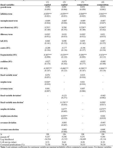
2.2. Results
In Table 1, we examine the effect of capital expenditures and the composition of public
expenditures on the probability of re-election. Regarding the macroeconomic variables, we
observe that the variable growth term is insignificantly related to re-election prospects in all
regressions, while the variable inflation term produces results that indicate a robust negative
effect on the probability of re-election. These results seem to verify the previous studies of
Alesina et al. (1998) and Brender and Drazen (2008), who found that voters dislike inflation
while the growth rate does not seem to affect re-election prospects. In general, studies for
developed countries are contradictory regarding the effect of the growth rate of output on
voting behaviour (see, e.g., Alesina and Rosenthal (1995)). As far as the variable
unemployment term is concerned, it turns out to be insignificantly related to re-election, in
line with most empirical evidence (see, e.g., Peltzman (1992); Aidt et al. (2011) and Alesina
et al. (2012)).
Variable illiteracy term is positive when statistically significant, reflecting that the
ability of the electorate to process available information can affect the incumbent's re-election
prospects. A possible explanation for this result is that the incumbent may have an advantage
in informing the voters, which may decrease with the level of voters education/sophistication.
Milligan et al. (2004) looking at the US and the UK find that more educated citizens appear
to have more information on candidates and campaigns. Our result may reflect that less
educated voters may rely more on a narrower set of sources of information influenced by the
incumbent (e.g., the "popular" media). The same may be true for less "experienced" voters,
which may explain the positive and statistically significant coefficient of the variable new
democracy in the majority of specifications in Table 1.22 The transition period to a
democratic regime may be complemented by an incumbency advantage due to a lower level
21 Pooled probit equations, though, yielded very similar qualitative results. 22
of political competition since it may take time to safeguard democratic principles (e.g.,
freedom of press) and to transform the political system (e.g., number of political parties). For
example, Keefer (2007) argues that, in younger democracies, political competitors are not
able to make broadly credible pre-electoral promises to voters.23
Regarding the government’s ideology, we obtain a positive but insignificant coefficient for the variable left, indicating that the probability of success is identical between
left-wing and right-wing governments (omitted category). The centre variable is negative and
insignificantly related to re-election prospects in Table 1. Although, in some other
(unreported) specifications centre seems to have a negative effect on re-election, this effect is
not robust. Moreover, variable fragmentation is negative and significantly related to
re-election prospects. This finding may reflect that ideologically fragmented governments are
more likely to face internal issues that can deteriorate the re-election prospects of the chief
executive in power. The coalition variable, on the other hand, is insignificantly related to
re-election prospects.24 Finally, we find that the probability of re-election is significantly lower
for the European Union members in the pre-EMU era after the enforcement of the Maastricht
treaty. The efforts of this group of countries to implement structural reforms before the
adoption of the common currency may have proven detrimental for the chief executives in
power.
Table 1 here
Turning now to the effect of fiscal performance over the whole term in office on
re-election prospects, in column (1) we find that the coefficient of capital expenditure is
marginally insignificant, while surplus term is positive and significant at the 10% level. This
result indicates that an increase of 1 percentage point in budget surplus as a share of GDP
over the whole term in office can improve the chances of re-election by about 2.6 percentage
points. On the contrary, in column (3) we find that all fiscal variables are insignificantly
related to the probability of re-election.
23
Besley and Part (2006) develop a model that allows for the possibility that the incumbent can influence the media through promises and threats. Their empirical evidence indicates that the length of the term of the chief executive or the party depends on media characteristics. Prior (2006) shows that the growth of television contributed to the rise in the incumbency advantage in U.S. through its effect on less-educated voters for whom television presented a new, less demanding source of news.
24 The variable coalition seems to be negatively and significantly related to re-election prospects only in the absence of the
As a next step, in columns (2) and (4) we split all fiscal variables in order to
disentangle the electoral effect of fiscal policy (fiscal variable deviation) versus the effect of
fiscal policy prior to the election year (fiscal variable non-election). As can be seen in
columns (2) and (4), electoral policies that affect public investment expenditures (capital
deviation) or the composition of public spending between capital and current expenditures
(composition deviation) do not affect re-election prospects. Existing empirical evidence for
the same sample of countries suggests that capital expenditures decrease during the election
period (see Katsimi and Sarantides (2012)).25 This finding indicates that an electoral fall in
capital expenditure does not affect voting behaviour. This result may be attributed to a
time-lag in the visibility of this type of expenditure during the election period. Capital
expenditures (e.g., infrastructure) are mostly long-term projects that will increase voters’
utility upon completion. Likewise, a change in the expenditure composition initiated by the
fall in capital expenditure may not affect voting behaviour, because this cut may not visible in
the election period. On the contrary, the variables capital election and composition
non-election, which capture policies prior to the election year, are positive and significantly
related to re-election.26 More specifically, an increase of 1 percentage point in capital
non-election (composition non-non-election) can increase the probability of re-non-election by 13.8 (3.0)
percentage points.27
Our results indicate that the timing of public capital spending is important for
incumbent's re-election: although both term average public investment as well as its level in
the election year does not seem to affect voting behaviour, capital spending in the years
before the electoral period does affect re-election probability. This implies that an incumbent
who wishes to maximize his re-election prospects should frontload public spending; he
should spend on capital as soon as he is elected in order to allow for a sufficient period for
this spending to be materialized and probably observed by voters while he should lower
25
As already mentioned, in the full specification of the budget constraint that we adopt, we choose as the omitted variable current expenditures but our results remain essentially the same if the omitted variable is total revenues.
26
A Wald test for the equality of coefficients between the variable capital (composition) deviation and capital (composition) non-election in columns (2) and (4) of Table 1 is performed. The value of the Wald test rejects the null of equal coefficients of variables capital (composition) deviation to the coefficient of capital (composition) non-election; the p-values are 0.09 and 0.10 for variables capital and composition, respectively.
27
capital spending in the final year of his term, when this type of spending is not rewarded by
voters.
Regarding the effect of total revenues and budget balances on re-election prospects,
the former, irrespective of the timing during the term in office, has no effect on the
probability of re-election.28 On the contrary, and in line with the findings of Brender and
Drazen (2008), we find that in developed economies, voters dislike deficits and even more so
if the deficit is perceived as electorally motivated. More specifically, in column (2) we
observe that a decrease of 1 percentage point in surplus non-election leads to a decrease of
about 3.9 percentage points in the chances of re-election. The impact of a deficit creation in
the election period is punished more heavily: a decrease of 1 percentage point in surplus
deviation leads to a decrease of about 7.7 percentage points in the chances of re-election.
Accordingly, Brender and Drazen (2008) showed that an increase of 1 percentage point in the
central government deficit can decrease the probability of re-election by 3-5 percentage
points, whereas an increase of 1 percentage point in the deficit during an election year
decrease the probability of re-election by 7-9 percentage points.29
3. Robustness
The main finding of the previous section is that, although voters seem to reward a high level
of public investment in the non-election years, a deviation in capital expenditure from this
level in the election year does not affect voting behaviour. In this section we want to test the
robustness of this result in the following ways: First, in Table 2 we re-estimate our
regressions by including capital expenditures and the composition of spending only for the
election year. Second, in Table 3 we conduct a battery of robustness checks on our main
regressions in columns (2) and (4) of Table 1, where we distinguish between electoral and
pre-electoral effects of fiscal policies. More specifically, we check if our results are affected
by the inclusion of country fixed effects. Moreover, we test if our results remain the same
when we adjust for the timing of elections. Furthermore, we modify the definition of the
dependent variable to follow more explicitly the party rather than leader re-election. Finally,
28
It should be noted that the qualitative results remain essentially the same after dropping revenues from our regressions.
29 Although the GFS does not provide data after 1999 for our main variables of interest which are capital and composition,
we distinguish between coalition and single-party cabinets, and we re-estimate our baseline
specification only for the latter. Due to space limitation only fiscal variables are reported in
Table 3.30
3.1. The level of fiscal policy and macroeconomic conditions around elections
Following previous studies, in our baseline specification in order to capture the electoral
effect of fiscal performance we use the deviation of election year value from the average
value of non-election years (see Veiga and Veiga (2007); Sakurai and Menezes-Filho
(2008)). According to the literature, the change rather than the level of fiscal policy variables
reflect better the impact of the incumbent on policy outcomes (see Brender and Drazen
(2008)). However, in Table 2 we test if including the level rather than the deviation of fiscal
variables in the election year affects our results (see, e.g., Jones et al. (2012)). Moreover, we
test if controlling for the impact of the macroeconomic variables in the election year may
affect the re-election prospects. We run the regressions including the level of fiscal and
macroeconomic variables in the election year, and not their term average or their non-
election years average for two reasons. First, when we calculate the average for the whole
term in office, we include the value of the election year. Second, the value of fiscal and
macroeconomic variables in the election year is highly correlated with the average in the
previous years of the term, which can significantly distort the results. Hence, in columns (1)
and (2) of Table 2, we re-run the regressions of columns (1) and (3) of Table 1, including the
value of fiscal and macroeconomic variables in the election year rather than the average value
of the whole term.
Table 2 here
As can be seen in Table 2, the level of public investment expenditures in the election year,
namely the variable capital, has no significant impact on re-election prospects. The same
holds also for the variables revenues and composition. However, in accordance with our
previous findings, the variable surplus affects significantly the probability of re-election.
Regarding macroeconomic conditions, once again only the inflation rate has a significant
negative impact on re-election prospects. Moreover, as far as the other control variables are
30
concerned, the qualitative results presented in Table 2 remain very similar to those depicted
in columns (1) and (3) of Table 1.
3.2. Country fixed effects
As already mentioned, the specification tests that we performed and the characteristics of our
panel induce us to use the pooled logit model as our basic specification. However, we want to
exclude the possibility that the results presented in Table 1 are driven by country specific
characteristics. Regarding our main variables of interest, if the share of investment
expenditures over GDP differs systematically between countries, and those countries with
higher shares of investment expenditures have more stable governments, then this would
certainly influence the estimation results. Therefore, in this sub-section we want to assess the
robustness of our results by introducing country fixed effects in our estimations. To do that
we apply the conditional logit model as proposed by Chamberlain (1980), which is the only
non-linear estimator designed for binary models, as in our case, which allows obtaining
consistent estimates through a fixed effects-like approach.31
As can be seen in the first two columns of Table 3, the inclusion of fixed effects does
not alter the statistical significance of our main variables of interest. More specifically,
capital deviation and composition deviation remain insignificant, capital non-election is
significant close at the 1% level, whereas variable composition non-election is significant at
the 10% level. Moreover, as before, variables surplus deviation and surplus non-election
have a statistically significant effect on re-election prospects.
3.3. The timing of elections
Regarding the timing of elections, the first check we perform is to exclude ‘early’ elections
from our sample, since they can introduce an important bias in our results. As argued by
Heckelman and Berument (1998), the timing of elections may not be exogenous but is chosen
strategically by the incumbent when economic conditions and the re-election probability are
favourable, raising issues of a reverse causation in our specification. Moreover, Rogoff
(1990) argues that, during predetermined elections, opportunistic incumbents have ample
time to use fiscal policy in order to increase re-election probabilities, far greater than in the
case of elections being called earlier. Consistent with that theoretical prediction, Katsimi and
31Two issues are worth noting here. First, the conditional logit estimator drops observations for Finland and France, because
Sarantides (2012) found that, only during predetermined elections, incumbents reduce capital
expenditures and shift the composition of expenditures towards public investment. Hence, in
line with Brender and Drazen (2005), we look at the constitutionally determined election
interval, and we keep in our sample those elections that are characterized as predetermined
and are held during the expected year of the constitutionally fixed term. As can be seen in
column (3) of Table 3, excluding early elections does not affect the statistical significance of
the variable capital non-election. More precisely, we observe that an increase of 1 percentage
point in capital non-election leads to an increase of about 11.9 percentage points in the
chances of re-election during predetermined elections. Although the value of the coefficient
of composition non-election in column (4) increases compare to the one reported in Table 1,
it becomes marginally insignificant. However, this result seems to be driven by the cases of
the predetermined elections where the leader does not spent the whole term in office. 32
Variable surplus loses its significance during predetermined elections. This is in direct
analogy with Brender and Drazen (2008), who also find that in predetermined elections their
result that voters punish election and pre-election year deficits in old democracies is not
robust. 33
One could further argue that an endogeneity bias can arise if an incumbent certain of
winning by a large margin may not manipulate expenditure, as in the case of a close race.
However, this source of endogeneity may not be important, since on the one hand, it is not
obvious why a strategy that helps re-election will only be followed by unpopular incumbents
(see Brender (2003)), and, on the other hand, even incumbents who are certain about their
re-election will still have an incentive to increase the number of the Parliament seats for their
party (see Veiga and Veiga (2007)).
32
It is worth noting that when we keep in the sample only the cases of the predetermined elections where the leader spent the whole term in office, coefficient of the variable composition non-election appears statistically significant whereas the coefficients of the variables capital non-election and composition non-election increase beyond the level of those depicted in Table 1. Moreover, when we attempt to capture the long term effect of public investment on re-election probability by including public investment in the first year of the term in office, our results indicate a positive impact of the initial public investment on the probability of re-election. Results available upon request.
33
Another form of endogeneity bias is that a known change in political majority may
affect public spending if the incumbent has different preferences over the level or the
composition of public spending than the opposition (see, among others, Persson and
Svensson (1989); Alesina and Tabellini (1990); and Milesi-Ferretti and Spolaore (1994)). In
our case, an incumbent with low popularity and a higher relative preference for current
expenditure than his opponent may raise this type of expenditure at the expense of capital
spending. Following Brender (2003), we attempted to minimize the possibility of an
endogeneity bias in the following ways: First, we tried to mitigate the effect of popularity on
public spending by controlling for the share of votes received in the previous elections. The
inclusion of this variable has no impact to our results and its coefficient is statistically
insignificant in every specification. Therefore, we exclude it from our specification.
Moreover, by looking at the data, we found very weak evidence suggesting that the most
unpopular incumbents adopted the largest cuts in public spending before elections in order to
improve their popularity. More specifically, in the case of single-party governments, we
found that, among the incumbents that decreased the capital to current expenditure ratio by
the largest amount, the highest percentage (55%) belonged in the middle of the distribution,
according to the share of votes they received, while 15% belonged in the upper quartile and
30% in the bottom quartile of our sample.34
Finally, one very important issue concerns the specific dates that elections took place
during the term in office. More specifically, in our specification the term in office starts after
the year that elections took place, and finishes in the election year of the end of the term.
However, one might argue that if the election was held in January, the newly elected
government can influence next year’s expenditures, while if elections were held later in the year, the incumbent may not had enough time to affect fiscal policy instruments. In order to
deal with this problem to the degree possible, we adjust our specification to take into account
whether elections took place in the first or in the second half of the year (see Vergne (2009)).
More specifically, if the election took place in the first half of the year, we define as election
year the year before the election. Alternatively, if the election took place in the second half of
the year, we define as election year the year of the election. For example if an election took
place in January 1990 and the next election in December 1993, in the new specification the
term is defined as the 1990-1993 period. On the contrary, if an election took place in
34
December 1990 and the next election in January 1993, the term is defined as 1991-1992. In
columns (5) and (6) of Table 3, we estimate regressions (2) and (4) of Table 1 after
re-adjusting our sample for this new definition of term and election year. As can be seen, the
qualitative results for fiscal variables capital and revenues are in line with those depicted in
Table 1. Once again, the effect of variable surplus becomes weaker.
Table 3 here
3.4. Party vs. leader re-election
The definition of the re-election variable in our baseline specification, which is broadly
consistent with the definition of Brender and Drazen (2008), is restricted in order to follow
the leader of the party in power until the election year. Although, in that way the re-election
variable allows for a clearer relationship between the leader and his/her policies, it does not
allow for a broader relationship between the party and its policies. Hence, at this point we set
the value of the re-election variable equal to 1 if the newly elected president/prime minister is
from the same party as the predecessor, irrespective of whether his predecessor quits in the
election year for whatever reason. As expected, in some cases the values of the two key
political variables deviate. Hence, when the leader in office resigns within the year of election
variable leader re-election takes value 0, while party re-election takes value 1 if the
successor leader comes from the same party and gets re-elected. By following parties that
have been in office for at least 2 years we have 115 campaigns in which the party in power
was re-elected in 71 cases. It is worth noting that the term in office is adjusted from
appointment to termination of parties rather than of individual leaders.
In columns (7) and (8) of Table 3, results for the variables capital and composition
and revenues are in line with those depicted in Table 1. Party re-election does not seem to be
affected by the level of deficit in the non-election year although our previous results indicate
that voters punish the leader of the party for a rise in deficit in the election year. This could
reflect the fact that when the leader in office resigns within the year of election and the
successor leader comes from the same party (variable leader re-election takes value 0, while
party re-election takes value 1) voters are more lenient in judging the policy choices of the
successor leader who has been in power for only a few months. The same holds for the
variable surplus deviation which becomes insignificant in column (7), while it is statistically
3.5. Single-party incumbents
Until now, we have included in our regressions observations in which the chief executive can
be the leader of a coalition, but also of a single-party government. The final robustness check
that we apply in our basic specification is to exclude from our regressions coalition
incumbents. Although until now we include a dummy variable to control for this category of
incumbents, we perform this check for two reasons. First, because, although our re-election
variable takes the value 0 in cases where the leader after the election comes from a different
party, this change can simply be a routine personnel replacement in a stable coalition
government (see Alesina et al. (2012)). Second, an interesting issue concerning this literature
is that coalition governments can be more heterogeneous and ‘vulnerable’ than single-party
governments (see, e.g., Alesina et al. (1997)), and as a consequence, they adopt different
fiscal policies raising issues of reverse causation in our specification (see, e.g., Roubini and
Sachs (1989); Perotti and Kontopoulos (2002)). Although when we drop coalition incumbents
from our estimations we are left with only 52 observations, given the issues related to
coalition incumbents, we find essential to follow the terms of individual leaders in office only
for the cases of single-party governments.
In columns (9) and (10) of Table 3, results indicate an even stronger connection
running from the variables capital/composition non-election to re-election prospects. More
precisely, we observe that an increase of 1 percentage point in capital non-election
(composition non-election) improves the probability of re-election by about 20.8 (4.2)
percentage points. Once again, the variable revenues is insignificantly related to re-election
prospects, whereas the variable surplus loses its significance.35
Concluding, the results of all robustness tests reported in Tables 2 and 3 indicate that
our basic results concerning the impact of public investment on an incumbent's re-election
chances are robust to a wide variety of different specifications performed in this section.
More specifically, all our results suggest that public investment in the non-election years is
rewarded by voters whereas its change, or its level, in the election year does not affect the
re-election probability. Moreover, in all specifications the level of revenues in the non-re-election
period as well as the electoral deviation of revenues does not seem to affect re-election
prospects. Finally, regarding the impact of deficits there is some very weak evidence for a
35 However, we should bear in mind that the low number of observations does not allow us a safe inference. For instance,
negative impact of deficits on re-election prospects in the non-election years whereas there is
mixed evidence about how the change in deficit in the election period affects voting
behaviour. Nevertheless, as in Brender and Drazen (2008), we find that in all specifications
deficit creation is not rewarded by voters in developed established democracies.
4. The Voting Function
Following previous studies in this area, we have so far examined the impact of fiscal and
economic performance on the probability of re-election using binary models (see, among
others, Brender (2003); Brender and Drazen (2008); Buti et al. (2010)). Although an
important strand of the literature examines the impact of fiscal and economic performance of
the vote share received by the incumbent (see, e.g., Peltzman (1992); Chappell and Veiga
(2000); Jones et al. (2012)) we chose the binary model as our basic specification in order to
be able to compare our results to the literature closest to our paper (see Brender and Drazen
(2008)). This set up allowed us to concentrate our attention on the determinants of the
probability that the incumbent will be re-elected. Many theoretical models with office
motivated politicians assume that incumbents maximize their re-election probability rather
than their popularity (see Rogoff (1990); Shi and Svensson (2006); Katsimi and Sarantides
(2012)). In the single party government framework assumed in these papers, a rise in the vote
share is equivalent to a rise in the re-election probability. However, in the case of coalition
governments, the incumbent party may manage to win a larger share of votes compared to
previous elections without being able to remain in power due to changes in the others parties’
numbers of seats.36 Thus, the binary framework may disregard important information
regarding voters' behaviour because, although incumbents can lose votes from one election to
another, they can still in some cases get re-elected. The significant advantage of the voting
function is its sensitivity to changes in popular support for incumbents (see Veiga (2013)).
Hence, our final step in this study is to investigate the effect of electoral and
pre-electoral policies on the vote share of the incumbent. Our dependent variable is the ratio of
the number of votes obtained by the incumbent party (or parties in case of coalition
incumbents) to the total number of valid votes in the current election. Alternatively, though,
we follow only the vote share received by the party of the chief executive in power.37 The
36
In our sample, we have 13 cases where the party of the chief executive gets a larger share of votes, whereas the popularity of the other parties that comprise the coalition government moves the opposite direction. However, in only 3 of these cases (Ireland 1987 and Sweden 1982, 1983) the chief executive was replaced.
37 For the second definition of the dependent variable we have two observations less than for the first definition, because in
homogeneity of the latter definition can reflect a clearer relationship between fiscal and
economic performance with the vote share. Additionally to the control variables we used in
the previous specifications, we follow common studies, and we include the vote share
obtained by the incumbent party (or parties in case of coalition incumbents) in the previous
election.
A drawback of this specification is that the vote share variable is bounded between 0
and 1 and therefore it does not satisfy the classic assumptions of the linear regression model.
If we simply use a linear estimation method, the estimated vote shares are not constrained to
lie within this interval. However, a simple logistic transformation of the dependent solves this
problem, making the dependent variable range from negative infinity to positive infinity,
eliminating predictions outside the allowable range (see, e.g., Veiga (2013)). Therefore, we
estimate the following equation:
(1)
In order to apply this transformation in our estimated equation, we choose to employ two
econometric models. First, we consider the fractional logit estimator, as proposed by Papke
and Wooldridge (2008). This is a quasi-maximum likelihood method that yields consistent
estimates when the dependent variable is bounded between 0 and 1. Second, we use the
logistic transformation of the dependent variable in the Ordinary Least Squares estimator
including country fixed effects so that to control for factors that remain constant over time.
Estimation results for equation (1) are shown in Table 4. It is worth noting that when
we estimate the vote function for the main incumbent party, our results indicate a stronger
effect of fiscal and economic performance on the vote share (see the right hand side of Table
4). Indeed, as expected, voters seem to consider the main incumbent party as more
responsible for economic policies and react to its decisions more consistently.
For our main variables of interest, capital and composition results are in line with
those depicted in the binary specification of the previous section. More specifically, variables
capital deviation and composition deviation are insignificantly related to the vote share in all
estimations. For the variable capital non-election, especially when related to the main
incumbent party, we get a robust positive effect. In columns (5) and (7), the results indicate