An Experimental and Theoretical Study of the Spin–Orbit Interaction for CO+(A 2Π3/2,1/2, v+=0–41) and O+2(X 2Π3/2,1/2g, v+=0–38)

Ames Laboratory Publications

Ames Laboratory

10-1999

An Experimental and Theoretical Study of the

Spin–Orbit Interaction for CO+(A 2Π3/2,1/2,

v+=0–41) and O+2(X 2Π3/2,1/2g, v+=0–38)

Dmitri G. Fedorov

Iowa State University

M. Evans

Iowa State University

Y. Song

Iowa State University

Mark S. Gordon

Iowa State University, [email protected]

C. Y. Ng

Iowa State University

Follow this and additional works at:

http://lib.dr.iastate.edu/ameslab_pubs

Part of the

Chemistry Commons

The complete bibliographic information for this item can be found at

http://lib.dr.iastate.edu/

ameslab_pubs/322

. For information on how to cite this item, please visit

http://lib.dr.iastate.edu/

howtocite.html

.

An Experimental and Theoretical Study of the Spin–Orbit Interaction for

CO+(A 2Π3/2,1/2, v+=0–41) and O+2(X 2Π3/2,1/2g, v+=0–38)

Abstract

Accurate spin–orbit splitting constants (Av+) for the vibrational levels v+=0–41 of CO+(A 2Π3/2,1/2) have

been determined in a rotationally resolved pulsed field ionization photoelectron study. A change in slope is

observed in the v+ dependence for Av+ at v+≈19–20. This observation is attributed to perturbation of the

CO+(A 2Π) potential by the CO+(B 2Σ+) state. Theoretical Av+ values for CO+(A 2Π3/2,1/2, v+=0–41)

have also been obtained using a newly developed

ab initio

computational routine for spin–orbit coupling

calculations. The theoretical Av+ predictions computed using this routine are found to be in agreement with

the experimental Av+ values for CO+(A 2Π3/2,1/2, v+=0–41). Similar Av+calculations obtained for O+2(X

2Π3/2,1/2g, v+=0–38) are also in accord with the recent experimental Av+ values reported by Song et al. [ J.

Chem. Phys.

111

, 1905 (1999)].

Keywords

Ab initio calculations, Field desorption

Disciplines

Chemistry

Comments

The following article appeared in

Journal of Chemical Physics

111 (1999): 6413, and may be found at

doi:

10.1063/1.479941

.

Rights

Copyright 1999 American Institute of Physics. This article may be downloaded for personal use only. Any

other use requires prior permission of the author and the American Institute of Physics.

An experimental and theoretical study of the spin–orbit interaction for CO + (A  2 Π

3/2,1/2 , v + =0–41) and O 2 + (X  2 Π 3/2,1/2g , v + =0–38)

D. G. Fedorov, M. Evans, Y. Song, M. S. Gordon, and C. Y. Ng

Citation: The Journal of Chemical Physics 111, 6413 (1999); doi: 10.1063/1.479941 View online: http://dx.doi.org/10.1063/1.479941

View Table of Contents: http://scitation.aip.org/content/aip/journal/jcp/111/14?ver=pdfcov

Published by the AIP Publishing

Articles you may be interested in

The Jahn-Teller effect in CH 3 Cl + ( X ̃ E 2 ) : A combined high-resolution experimental measurement and ab initio theoretical study

J. Chem. Phys. 136, 064308 (2012); 10.1063/1.3679655

Theoretical investigation of vibronic and spin-orbit effects in the ground X 2Πu electronic state of the dicyanoacetylene cation

J. Chem. Phys. 135, 024314 (2011); 10.1063/1.3608913

Photoelectron spectroscopic study of the E⊗e Jahn–Teller effect in the presence of a tunable spin–orbit interaction. I. Photoionization dynamics of methyl iodide and rotational fine structure of CH3I+ and CD3I+

J. Chem. Phys. 134, 054308 (2011); 10.1063/1.3547548

Rovibrationally selected and resolved pulsed field ionization-photoelectron study of propyne: Ionization energy and spin-orbit interaction in propyne cation

J. Chem. Phys. 128, 094311 (2008); 10.1063/1.2836429

Unimolecular decay pathways of state-selected CO 2 + in the internal energy range of 5.2–6.2 eV: An experimental and theoretical study

J. Chem. Phys. 118, 149 (2003); 10.1063/1.1524180

An experimental and theoretical study of the spin–orbit interaction

for CO

ⴙ

„

A

2

⌸

3/2,1/2

,

v

ⴙ

ⴝ

0 – 41

…

and O

2ⴙ

„

X

2

_⌸

3/2,1/2g

,

v

ⴙ

ⴝ

0 – 38

…

D. G. Fedorov, M. Evans, Y. Song, M. S. Gordon, and C. Y. Nga)

Ames Laboratory, USDOE and Department of Chemistry, Iowa State University, Ames, Iowa 50011 共Received 10 June 1999; accepted 14 July 1999兲

Accurate spin–orbit splitting constants (A_v⫹) for the vibrational levels v⫹⫽0 – 41 of CO⫹(A2⌸3/2,1/2) have been determined in a rotationally resolved pulsed field ionization photoelectron study. A change in slope is observed in the v⫹ dependence for A_v⫹ at v⫹

⬇19– 20. This observation is attributed to perturbation of the CO⫹(A2⌸) potential by the CO⫹(B2⌺⫹) state. Theoretical A_v⫹ values for CO⫹(A2⌸3/2,1/2,v⫹⫽0 – 41) have also been obtained using a newly developed ab initio computational routine for spin–orbit coupling calculations. The theoretical A_v⫹ predictions computed using this routine are found to be in agreement with the experimental A_v⫹ values for CO⫹(A2⌸3/2,1/2,v⫹⫽0 – 41). Similar Av⫹

calculations obtained for O₂⫹(X2⌸3/2,1/2g,v⫹⫽0 – 38) are also in accord with the recent experimental A_v⫹ values reported by Song et al. 关J. Chem. Phys. 111, 1905 共1999兲兴. © 1999

American Institute of Physics. 关S0021-9606共99兲00938-1兴

I. INTRODUCTION

The spin–orbit constants (A_v⫹) for the v⫹⫽0 and 2 vibrational levels of CO⫹(A2_⌸

3/2,1/2) have been determined to be 122.0 and 121.87 cm⫺1, respectively,1,2 which are higher than the value of 117.5 cm⫺1 cited in Huber and Herzberg3 based on earlier measurements. To our knowl-edge, the A_v⫹ values for the high v⫹-levels of CO⫹(A2⌸3/2,1/2,v⫹) have not been measured.

The most general experimental method for the determi-nation of A_v⫹values of cations for a wide range ofv⫹levels is the photoelectron spectroscopic technique. Due to autoion-ization mechanisms, photoelectron spectroscopic measure-ments often allow the observation of highly vibrationally ex-cited states for the cation.4,5 This is especially the case for threshold photoelectron共TPE兲or pulsed field ionization pho-toelectron共PFI-PE兲measurements using a tunable ionization source,5where highly vibrational excited ionic states can be observed due to finite couplings to nearby resonance Ryd-berg states and/or repulsive states. In photoionization studies using a fixed energy light source, such as HeI, highly vibra-tionally excited ionic states with negligible Franck–Condon factors can also be observed.4When the HeI photon energy coincides with the excitation energy of a Rydberg level, the Rydberg level initially formed can decay to a lower vibronic state of the cation, concomitant with the ejection of an ener-getic electron. This two-step mechanism can thus give rise to a long progression of vibrational bands for the cation, which would not be observed via direct ionization. The HeI spec-trum for CO obtained by Wannberg et al.4 indeed reveals high vibrational bands up tov⫹⫽18 for CO⫹(A2⌸). How-ever, the two spin–orbit states cannot be resolved in the lat-ter experiment due to the relatively small spin–orbit splitting constant (A_v⫹) for CO⫹(A2⌸3/2,1/2). Kong and Hepburn6

have recently performed a high-resolution vacuum ultravio-let 共VUV兲 laser PFI-PE study of CO⫹(A2⌸3/2,1/2,v⫹

⫽0 and 1). The observed rotationally resolved PFI-PE spec-tra for these vibrational bands are found to be consistent with

A_v⫹⫽120 cm⫺1forv⫹⫽0 and 1, which is close to the value of 122 cm⫺1 determined previously.1,2

Taking advantage of the high-resolution vacuum ultra-violet 共VUV兲 facility of the chemical dynamics beamline established at the advanced light source 共ALS兲,7,8 we have recently developed a novel synchrotron based PFI-PE detec-tion scheme,9,10 achieving PFI-PE resolutions similar to that observed in VUV laser PFI-PE studies.10–12The ease of tun-ability over a wide energy range 共6–30 eV兲 has made this synchrotron based PFI-PE method highly productive, par-ticularly in measuring photoelectron bands of a long vibra-tional progression. In recent studies, we have reported rota-tionally resolved PFI-PE bands for long progressions of O₂⫹(X2⌸_3/2,1/2g,v⫹⫽0 – 38),13 NO⫹(X1⌺⫹,v⫹⫽0 – 32),14 and CO⫹(X2⌺⫹,v⫹⫽0 – 42).15Using the same experimen-tal method, we have obtained rotationally resolved PFI-PE spectra for CO⫹(A2⌸3/2,1/2,v⫹⫽0 – 41). The intensities of PFI-PE bands for higher v⫹ 共⬎10兲 levels of CO⫹(A2⌸3/2,1/2) are more than 100 fold lower than those observed for thev⫹⫽0 – 2 bands. Despite the low intensities for the high v⫹ bands, we have successfully recorded most of the PFI-PE bands for CO⫹(A2⌸3/2,1/2,v⫹⫽0 – 41) at the rotationally resolved level with good signal-to-noise ratios. Here, we present accurate A_v⫹ values for CO⫹(A2⌸3/2,1/2,v⫹⫽0 – 41) derived from the analysis of the rotationally resolved PFI-PE spectrum of CO.

In the theoretical front, reliable calculations on spin– orbit interactions have not been readily accessible due to the requirement of accurate electronic and vibrational wave functions. Many theoretical calculations16–19have been made a兲_{Electronic mail: [email protected]}

JOURNAL OF CHEMICAL PHYSICS VOLUME 111, NUMBER 14 8 OCTOBER 1999

6413

0021-9606/99/111(14)/6413/9/$15.00 © 1999 American Institute of Physics

on the potential-energy surfaces of CO⫹. The recent multi-configuration self-consistent field multi-configuration interaction

共MCSCF-CI兲 calculations of Lavendy and Robbe16 and Okada and Iwata17 have obtained reliable predictions for the vibrational and rotational constants of CO⫹(A2⌸3/2,1/2). However, the A_v⫹ value of 92 cm⫺1 for CO⫹(A2⌸3/2,1/2) calculated by Lavendy and Robbe16 is significantly smaller than the experimental measurements1,2of 122 cm⫺1.

In view of the lack of computational routines available for reliable calculations of spin–orbit coupling constants, we have recently developed a new ab initio computational code for this purpose. This code, to be included into the produc-tion version of the publicly available quantum chemistry packageGAMESS,20has the capability of performing efficient spin–orbit coupling calculations for arbitrary spin multiplici-ties with any CI wave function types supported byGAMESS, for both one and two electron spin–orbit coupling operators. As a test of this computational code, we have calculated the

A_v⫹values for CO⫹(A2⌸3/2,1/2,v⫹⫽0 – 41) for comparison with the experimental measurements.

Highly accurate spin–orbit coupling constants for O₂⫹(X2⌸1/2,3/2g,v⫹⭐11) have been determined pre-viously21 in a comprehensive analysis of the O₂⫹(A2⌸u) →O₂⫹(X2⌸g) emission system. The VUV laser PFI-PE study of Kong and Hepburn has extended the measurement to O₂⫹(X2⌸1/2,3/2g,v⫹⫽24).22We note that the Av⫹values

for O₂⫹(X2⌸_1/2,3/2g,v⫹⫽⫺0 – 45) has also been reported re-cently in a synchrotron based TPE study.23 However, the latter A_v⫹ values are derived only from vibrationally re-solved data. By employing the synchrotron based PFI-PE detection method, Song et al. have made a comprehensive spectroscopic study on O₂⫹(X2⌸_1/2,3/2g,v⫹⫽⫺0 – 38) at the rotational-resolved level,13which provides accurate A_v⫹ val-ues for these states. Thus, the experimental A_v⫹ values for O₂⫹(X2_⌸

1/2,3/2g) can be considered well established. For this reason, we have also obtained theoretical A_v⫹values for this system. The comparison of the theoretical values with ex-perimental A_v⫹ data for the O₂⫹(X2_⌸

1/2,3/2g) system serves as a second test case for the new computational code.

II. EXPERIMENTAL AND THEORETICAL METHODS A. High-resolution PFI-PE measurements

The design and performance of the chemical dynamics beamline at the ALS has been described previously.7–11 Briefly, the major components for the high-resolution VUV photoionization facility at this beamline include a 10 cm pe-riod undulator (U10), a gas harmonic filter,24 a 6.65 m off-plane Eagle mounted monochromator,8and a photoelectron– photoion apparatus.9–11

In the present experiment, helium was used in the gas harmonic filter, where higher undulator harmonics with pho-ton energies greater than 24.59 eV were suppressed. The fundamental light from the undulator was then directed into the 6.65 m monochromator and dispersed by a 4800 l/mm grating (dispersion⫽0.32 Å/mm) before entering the experi-mental apparatus. The ALS storage ring is capable of filling 328 electron buckets in a period of 656 ns. Each electron bucket emits a light pulse of 50 ps with a time separation of

2 ns between successive bunches. In each storage ring pe-riod, a dark gap共80 ns兲consisting of 40 consecutive unfilled buckets exists for the ejection of cations from the orbit. Thus, the present experiment was performed in the multi-bunch mode with 288 multi-bunches in the synchrotron orbit, cor-responding to a repetition rate of 439 MHz.

The multipurpose photoelectron–photoion apparatus as-sociated with the chemical dynamics beamline was used for the present study.9–11 A continuous effusive CO beam was produced by a metal orifice (diameter⫽0.5 mm) at 298 K and a distance of 0.5 cm from the photoionization– photoexcitation 共PI/PEX兲 region. Thus, the rotational tem-perature of the CO sample is expected to be ⬇298 K. We estimate that the CO density at the PI/PEX region is

⬇10⫺3_{Torr. The photoionization chamber and} photoelec-tron chamber were evacuated by turbomolecular pumps with pumping speeds of 1200 and 3400 L/s, respectively. The respective pressures maintained in the photoionization cham-ber and the photoelectron chamcham-ber were ⬇1⫻10⫺5 and

⬇1⫻10⫺7Torr during the experiment.

The PFI-PE detection scheme using the high-resolution monochromatized undulator synchrotron radiation facility at the ALS has been described previously.9–11Briefly, a pulsed electric field (height⫽1.1 V/cm, width⫽40 ns, delayed by 20 ns with respect to the beginning of the 80 ns synchrotron dark gap兲 was applied to the repeller at the PI/PEX region. This pulsed electric field was used to field ionize high-n Rydberg species and extract photoelectrons toward the detec-tor and was applied every synchrotron ring period 共0.656 ␮s兲. An electron spectrometer, which consists of a steradi-ancy analyzer and a hemispherical energy analyzer arranged in tandem, was used to filter prompt electrons. We have pre-viously shown that PFI-PEs can be detected with little back-ground from prompt electrons after only an 8 ns delay with respect to the beginning of the dark gap.

The achievable PFI-PE resolution depends on the reso-lution of the excitation VUV light source and the magnitude of the applied pulsed electric field.10The PFI-PE spectra for CO presented in this experiment were measured using mono-chromator slits ranging from 30–200 ␮m. The PFI-PE reso-lution achieved was 4–7 cm⫺1 关full width at half maximum

共FWHM兲兴. The photon energy step size and counting time used at each photon energy varied between 0.1–0.3 meV and 3–30 s, respectively.

The PFI-PE spectra for CO were calibrated using the PFI-PE spectra of the Ar⫹(2P3/2) and Ne⫹(2P3/2) bands ob-tained at the same experimental conditions. This calibration scheme assumes that the Stark shifts for the IEs of CO and the rare gases are identical. The calibration for the CO PFI-PE spectrum was made before and after the experiment. Our previous experience with energy calibrations of the PFI-PE spectra of other molecular systems indicates that the accuracy of the present energy calibration is within ⫾0.5 meV.25 Since the spin–orbit PFI-PE components for indi-vidualv⫹-levels were recorded in a single scan, the error due to energy calibration does not apply to the uncertainties as-signed for the A_v⫹values. Most of the A_v⫹ values reported here are based on rotationally resolved data and have uncer-tainties well within ⫾2 cm⫺1.

6414 J. Chem. Phys., Vol. 111, No. 14, 8 October 1999 Fedorovet al.

B. Spin–orbit coupling calculations

Ab initio spin–orbit coupling calculations have been

made possible by generalization of the existing spin–orbit coupling code built into the quantum chemistry package GAMESS.20In order to accurately reproduce experimental re-sults, a large basis set 共AVTZ, built intoMOLPRO兲26–30and an extensive CI wave function have been used. The orbitals are optimized with complete active space self-consistent field

共CASSCF兲method, the active space including electrons in 8 orbitals (2s and 2 p on C and O兲.31Energy values are further refined with single and double excitations from the CASSCF active space into the virtual space using MOLPRO. We have examined the effect of adding single and double excitations from the core 1s orbitals into virtual space: The CO⫹results do not include such excitations and the O2⫹results do. Spin– orbit coupling calculations are performed with the CASSCF wave function and Pauli–Breit Hamiltonian,32including rig-orous one and two-electron terms and using the modified version ofGAMESSsoon to be released for distribution. The effect of including neighboring states into spin–orbit cou-pling diagonalization has been studied. CO⫹calculations in-clude the 6 lowest CI roots and O₂⫹calculations include two roots共i.e., only the2_⌸

u state兲.

The potential energy of CO⫹(A2⌸) has been calculated for a series of internuclear C–O distances共R兲of interest and a geometry optimization has been performed 共at the CASSCF level兲to locate the potential minimum. Experimen-tally, the splitting between the CO⫹(A2⌸3/2) and CO⫹(A2⌸1/2) spin–orbit states is found as a function of vibrational quantum number up to v⫹⫽41. The rotational constants (B_v⫹) for CO⫹(A2⌸3/2,1/2,v⫹⫽0 – 41) have also been determined. In the first approach, the corresponding average R value

具

r_␯⫹

典

for individual v⫹-levels of CO⫹(A2⌸) is estimated using the approximation

具

r_␯⫹

典

⫽ ប

冑

2␮B_␯⫹, 共1兲

where B_v is the rotational constant given by the experiment and␮is the reduced mass of CO⫹. At each

具

r_␯⫹

典

value, the spin–orbit coupling constant is computed 共the single-point approach兲. As shown in the discussion below, the A_v⫹

con-stants for CO⫹(2⌸3/2) and CO⫹(2⌸1/2) calculated at these

具

r_␯⫹

典

distances deviate significantly from the experimental values, especially for highv⫹ levels.

A more sophisticated approach involves the least-square fit of the calculated ab initio potential energies at a series of

R values to a Morse potential

U共R兲⫽De兵1⫺exp关⫺a共R⫺Re兲兴其2, 共2兲

where De is the well-depth and Re is the internuclear dis-tance at the potential minimum. The best fitted parameters

Deand a obtained for the Morse potential are listed in Table I. The corresponding vibrational frequency (␻e) and anhar-monicity constant (␻e␹e) for the Morse potential, together with the ab initio Revalue for CO⫹(A2⌸3/2,1/2,v⫹⫽0), are also included in Table I. We note that for a Morse potential only two out of the four parameters (De, a,␻e,␻e␹e) are independent. Since accurate vibrational energies for the CO⫹(A2⌸3/2,1/2,v⫹⫽0 – 41) states have also been deter-mined based on the simulation of their PFI-PE bands, we have also constructed a Morse potential to provide the best fit for the experiment vibrational energies of CO⫹(A2⌸3/2,1/2). The best fitted parameters for the experi-mental CO⫹(A2⌸3/2) and CO⫹(A2⌸1/2) Morse potentials are also given in Table I. We find that these Morse potentials obtained based on the experimental vibrational energies for CO⫹(A2_⌸

3/2,1/2) are in reasonable agreement with the CO⫹(A2_{⌸) Morse potential based on the ab initio} calcula-tion. We note that the R_evalue and the width of the theoret-ical CO⫹(A2⌸) Morse potential are greater than the experi-mental CO⫹(A2⌸_3/2,1/2) Morse potentials. As a result, the outer turning point of the theoretical Morse potential is greater than that of the experimental Morse potential at the same energy. We also list the Morse potential parameters for CO⫹(A2⌸) constructed based on the vibrational constants cited in Huber and Herzberg.3 These parameters are in ac-cord with those deduced from the present experiment.

The vibronic wave function used is

⌿␯_{共r,R兲⫽⌿}

N

␯_共R兲⌿

e共r,R兲, 共3兲

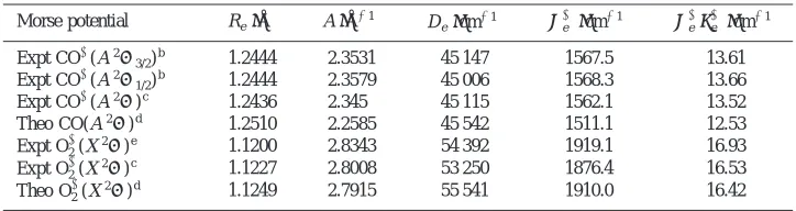
[image:6.612.125.487.74.170.2]

where ⌿_N␯(R) is an eigenfunction of the theoretical Morse TABLE I. Parametersa_{for the Morse potential关Eq.共2兲兴for CO}⫹_(A2_{⌸) and O}

2

⫹_(X2_{⌸) obtained by fitting the} ab initio potential energies and experimental vibrational energies for CO⫹(A2_⌸3/2).

Morse potential Re共Å兲 A共Å⫺1兲 De共cm⫺

1

兲 ␻e⫹共cm⫺

1_{兲 ␻}

e

⫹_␹

e

⫹_共cm⫺1_兲

Expt CO⫹(A2_⌸3/2)b _{1.2444 2.3531 45 147 1567.5 13.61}

Expt CO⫹(A2_⌸1/2)b _{1.2444 2.3579 45 006 1568.3 13.66}

Expt CO⫹(A2_⌸)c _{1.2436 2.345 45 115 1562.1 13.52}

Theo CO(A2_⌸)d _{1.2510 2.2585 45 542 1511.1 12.53}

Expt O2⫹(X2⌸)e 1.1200 2.8343 54 392 1919.1 16.93

Expt O2⫹(X2_⌸)c

1.1227 2.8008 53 250 1876.4 16.53

Theo O2⫹(X

2_⌸)d _{1.1249 2.7915 55 541 1910.0 16.42}

a_R

eis the equilibrium bond distance for CO⫹(A2⌸,v⫹⫽0) and De⫽well depth,␻e⫹⫽vibrational frequency,

and␻e⫹␹e⫹⫽anharmonicity for the Morse potential.

b_{Morse potential based on experimental vibrational energies for work.} c

Morse potential based on vibrational constants cited in Ref. 3.

d_{Morse potential based on ab initio potential energies calculated in this work.} e_{Morse potential based on experimental vibrational energies of Ref. 13.}

6415 J. Chem. Phys., Vol. 111, No. 14, 8 October 1999 Spin-orbit interaction for CO⫹

potential, ⌿_e(r,R) is the electronic wave function, and r is the electron coordinate. The theoretical A_v⫹ value is calcu-lated as,

A_v⫹⫽

冕 冕

⌿_N␯共R兲⫹关⌿_e共r,R兲⫹Hˆ_PB⌿_e共r,R兲

⫺⌿e

⬘共

r,R兲⫹HˆPB⌿e

⬘共

r,R兲兴⌿N␯共R兲drdR

⫽

冕

⌿N␯共R兲⫹A共R兲⌿N␯共R兲dR, 共4兲

where HˆPB is the Pauli–Breit 共PB兲 Hamiltonian31 and

⌿e(r,R) and⌿e

⬘

(r,R) are the eigenvectors of the HPB ma-trix in the basis of CASSCF states. The unprimed and primed states correspond to the two levels between which the split-ting is calculated 共i.e., between J⫽12 and J⫽

3

2 levels兲.

Ab initio splitting constants as a function of R, A(R), are first

calculated at discrete R values and then fitted to an appropri-ate analytical form for the convenience of performing nu-merical integration. For the CO⫹(A2⌸3/2,1/2) system, the

A(R) function is found to have the form A(R)⫽h(1 ⫺tanh关(R⫺R0)s兴)⫹A0with the following least-square fit pa-rameters: h⫽51.25, A0⫽13.5, R0⫽2.02, s⫽3.75. Here, R and A(R) are in Å and cm⫺1, respectively.

The average vibrational energies for the O₂⫹(X2⌸3/2,1/2g) spin–orbit states have been determined recently in a similar PFI-PE experiment by Song et al.13 The Morse potentials based on fitting to these experimental vibrational energies are given in Table I for comparison with the best fitted

ab initio Morse potential for O₂⫹(X2⌸). As a reference, we also include in Table I the Morse potential for O₂⫹(X2⌸) based on the vibrational constants cited in Huber and Herzberg.3 Similar to the observation for the CO⫹(A2⌸) system, the theoretical Re value is larger than that deter-mined in the experiment. As a result, the other wall of the theoretical Morse potential for O₂⫹(X2⌸) is wider than that for the experimental Morse potential.

The A(R) function associated with Eq. 共4兲 of the O₂⫹(X2⌸) system has the functional form: A(R) ⫽h exp关⫺s(R⫺R0)2兴⫹A0. The least-square fit parameters are, h⫽138.219, A0⫽1.06641, R0⫽1.0115, and s

⫽58.9876.

III. RESULTS AND DISCUSSION A. COⴙ„A2_⌸

3/2,1/2,vⴙⴝ0 – 41…

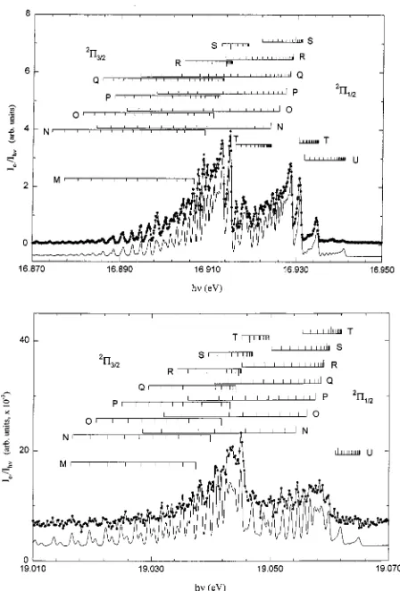
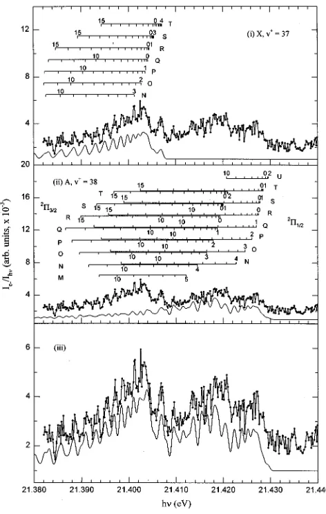
We have obtained rotationally resolved PFI-PE bands for CO⫹(A2⌸3/2,1/2,v⫹⫽0 – 41). The bulk of these data and their analysis, including important issues on spectroscopy and photoionization dynamics, will be presented in a future publication.33 Here, we have selected to show in Figs. 1共a兲, 1共b兲, and 2共b兲 the respective experimental PFI-PE bands

共solid circles兲 for CO⫹(A2⌸3/2,1/2,v⫹⫽2,15,38) to illus-trate of the assignment for the spin–orbit components and the typical quality of the simulation. As with the rotational and vibrational constants, the A_v⫹ values for CO⫹(A2⌸3/2,1/2,v⫹⫽0 – 41) are derived from the spectral simulation. The intensities shown for the spectra of Figs. 1共a兲, 1共b兲, and 2 reflect the actual relative intensities. As

shown in these figures, the intensities for the CO⫹(A2⌸3/2,1/2,v⫹⫽15 and 38) bands are more than two orders of magnitude lower that for the CO⫹(A2⌸3/2,1/2,v⫹

⫽2) band. We note that the PFI-PE band for CO⫹(A2⌸3/2,1/2,v⫹⫽38) has partial overlap with the CO⫹(X2⌺⫹,v⫹⫽37). Thus, Fig. 2 is a composite figure with panel 共a兲 showing the comparison of the experimental

共solid circles兲 and simulated 共solid line兲 spectra for CO⫹(X2⌺⫹,v⫹⫽37). The analysis and simulation of the PFI-PE bands for CO⫹(X2⌺⫹,v⫹⫽0 – 42) has been re-ported previously and thus will not be substantiated here.13

The relative intensities for rotational structures resolved in a vibrational band were simulated using the Buckingham– Orr–Sichel 共BOS兲 model,34 which is described by the for-mula

[image:7.612.325.549.49.380.2]

␴共J⫹←N

⬙

兲⬀⌺_␭Q共␭;J⫹,N

⬙

兲C_␭. 共5兲 This model was derived to predict rotational line strengths observed in the single-photon ionization of diatomic mol-ecules. Since the BOS model does not take into account channel interactions, which are certain to occur in the FIG. 1. Comparison of the experimental共solid circles兲and BOS simulated

共solid line兲 PFI-PE spectra for 共a兲 CO⫹(A2_⌸

3/2,1/2,v⫹⫽2) and 共b兲

CO⫹(A2_⌸

3/2,1/2,v⫹⫽15). Positions for individual rotational are indicated

using down pointing and up pointing stick marks for the 2_⌸

3/2and2⌸1/2

components, respectively. The rotational branches are labeled as M, N, O, P,

Q, R, S, T, and U for⌬N⫽⫺4,⫺3,⫺2,⫺1, 0, 1, 2, 3, and 4, respectively. In each⌬N case shown, the position of the first and second transitions are

indicated by progressively shorter lines. The PFI-PE resolution achieved ⫽4 cm⫺1_共FWHM兲.

6416 J. Chem. Phys., Vol. 111, No. 14, 8 October 1999 Fedorovet al.

PFI-PE spectra, we may consider the BOS simulation used here as semiempirical in nature. As in previous studies, the BOS simulation is valid in determining spectroscopic con-stants from the experimental PFI-PE spectra. The factor C_␭ is associated with the electronic transition moments, which is the linear combination of electron transition amplitudes for the possible angular momenta l of the ejected electron. The other factor Q is determined by the angular momentum cou-pling scheme. The parameter ␭ can be interpreted as the partial wave of the electron in the ground state of the neutral molecule. The more general interpretation of␭is that of the angular momentum transfer in the photoionization process. The angular momentum coupling factor Q for the

photoion-ization of the present CO system can be described by a Hund’s case 共b兲 to 共a兲 transition. The Q factor is thus ex-pressed as

Q共␭;J⫹,N

⬙兲

⫽2J

⫹_⫹1

2S⫹⫹1_␹⫽兩

兺

_␭⫺1/2兩

␹⫽␭⫹1/2

共2␹⫹1兲

⫻

冉

␭ S

⫹ _␹

⌬⌳ ⌺⫹ _⌳⬙⫺⍀⫹

冊

2

⫻

冉

J

⫹ _{␹ N}

_⬙

⫺⍀⫹ _⍀⫹_{⫺⌳⬙ ⌳⬙}

冊

2

, 共6兲

where ⌬⌳⫽⌳⫹⫺⌳⬙ and ⍀⫹⫽兩⌳⫹⫾⌺⫹兩. Here, ⌳⫹ and

⌺⫹_{are the projection of the electron orbital angular}

momen-tum and electron spin angular momenmomen-tum on the axis of CO⫹, respectively, and⌳⬙ is the projection of the electron orbital angular momentum on the axis of CO. Given that

⌬⌳⫽1 for the transition CO⫹(A2_⌸

⍀,v⫹)

←CO(X1_⌺⫹_,v

_⬙

_{⫽0), the first 3- j symbol of Eq. 共6兲} re-quires that ␭⭓1. The contribution by each C_␭ was deter-mined from the fit to the experimental data. Each spin–orbit state was simulated using a unique set of C_␭’s. The rotational structure observed in the experiment was accounted for using the BOS coefficients (C1, C2, C3, and C4). Thus, the pos-sible angular momentum states for the ejected photoelectron were l⫽0, 1, 2, 3, 4, and 5. The possible change in total angular momentum for a Hund’s case 共b兲 to共a兲 ionization transition is given by12

⌬J⫽J⫹⫺J

⬙

⫽l⫹3 2,l⫹

1

2,...,⫺l⫺ 3

2. 共7兲

Rotational transitions (⌬N⫽N⫹⫺N

⬙

) of⫺4,⫺3,⫺2,⫺1, 0, 1, 2, 3, and 4共designated as M, N, O, P, Q, R, S, T, and U branches, respectively兲 are clearly observed in the spectra, although transitions up to⌬N⫽⫾6 are possible according to Eq. 共7兲.

We assume that the rotational population for CO was characterized by a Boltzmann distribution with a rotational temperature of 298 K. The simulation uses known spectro-scopic constants for the molecular ground-state CO(X1⌺⫹,v⫹):␻e

⬙

⫽2169.813 58 cm⫺1, ␻e␹e

⬙

⫽13.288 31 cm⫺1_{, B} e

⬙

⫽1.931 28 cm⫺1_{, and ␣e}

⬙

⫽0.0175 04 cm⫺1_.3 _{The spin-rotational splitting present in} the ionic state has been ignored since it is much smaller than the experimental PFI-PE resolution.

In addition to the BOS C_␭ coefficients, the rotational constant B⫹_v and the spin–orbit coupling constant A_v⫹ were varied during the simulation of each vibration level. The simulated spectra 共solid line, lower spectra兲 shown in Figs. 1共a兲, 1共b兲, and 2共b兲were obtained using a Gaussian profile with a linewidth of 4, 4, and 7 cm⫺1共FWHM兲, respectively. The positions of the rotational transitions CO⫹(A2⌸3/2, v⫹,N⫹)←CO(X1⌺⫹,v

⬙

⫽0, N

⬙

) and CO⫹(A2⌸1/2, v⫹,N⫹)←CO(X1⌺⫹,v

⬙

⫽0, N

⬙

) are shown by, respec-tively, downward pointing and upward pointing stick marks in Figs. 1共a兲, 1共b兲, and 2共b兲. As shown in Figs. 1共a兲and 1共b兲, the agreement between the BOS simulated spectra and the experiment PFI-PE spectra are excellent, yielding values of 120.2⫾2.0 cm⫺1 for A_v⫹(v⫹⫽2), and 117.0⫾2.0 cm⫺1for

A_v⫹(v⫹⫽15). The A_v⫹(v⫹⫽2) value is in excellent accord FIG. 2. Composite simulation spectra for CO⫹(X2_⌺⫹_,v⫹_{⫽37) and}

CO⫹(A2⌸,v⫹⫽38). The figure is divided into three panels. Panel共i兲 关共ii兲兴 compares the experimental PFI-PE spectrum共solid circles兲and the deconvo-luted 共solid line兲 PFI-PE spectrum for CO⫹(X2⌺⫹,v⫹⫽37)

关CO⫹(A2_⌸

3/2,1/2,v⫹⫽38)兴. Panel共iii兲compares the experimental共solid

circles兲 PFI-PE spectrum with the sum of the deconvoluted共solid line兲 spectra for CO⫹(X2_⌺⫹_,v⫹_{⫽37) and CO}⫹_(A2_⌸

3/2,1/2,v⫹⫽38). In panel

共i兲, positions for individual rotational transitions are indicated by down pointing stick marks. In panel共ii兲, positions for individual rotational transi-tions are indicated using down pointing and up pointing stick marks for the

2_⌸

3/2and2⌸1/2components, respectively. The numbers in panels共i兲and共ii兲

are N⬙values. The rotational branches are labeled as M, N, O, P, Q, R, S, T, and U for⌬N⫽⫺4,⫺3,⫺2,⫺1, 0, 1, 2, 3, and 4, respectively. The PFI-PE resolution achieved⫽4 cm⫺1_共FWHM兲.

6417 J. Chem. Phys., Vol. 111, No. 14, 8 October 1999 Spin-orbit interaction for CO⫹

[image:8.612.58.294.52.424.2]

with the literature value of 121.87 cm⫺1.2The comparison of the BOS simulated 共solid line兲 and experimental 共solid circles兲 PFI-PE band for CO⫹(A2_⌸

1/2,v⫹⫽38) is shown in Fig. 2共b兲. The sum of the simulated spectra for CO⫹(X2⌺⫹,v⫹⫽37) shown in Fig. 2共a兲 and CO⫹(A2⌸_1/2,v⫹⫽38) gives the overall simulated spectrum

共solid line兲 in Fig. 2共c兲, which is again in excellent accord with the experimental PFI-PE spectrum 共solid circles兲. The

A_v⫹value for CO⫹(A2⌸3/2,1/2,v⫹⫽38) is determined to be 66.1⫾3.0 cm⫺1.

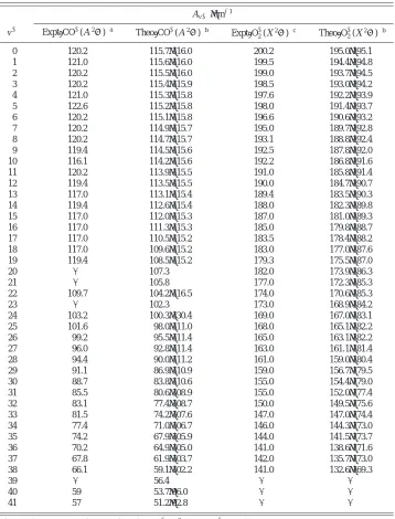
The A_v⫹values for CO⫹(A2⌸1/2,v⫹⫽0 – 41) obtained in the BOS simulation are listed in Table II. The plot of the

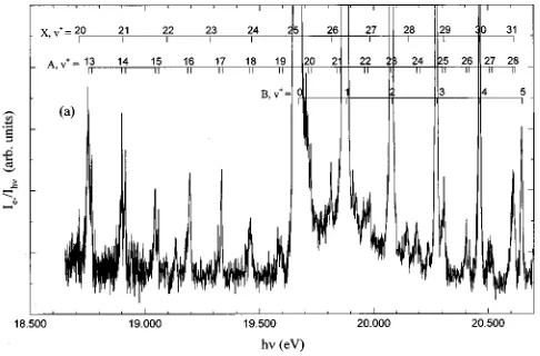
experimental A_v⫹ value versusv⫹ is shown in Fig. 3. It is interesting to note that the A_v⫹value seems to remain nearly constant until v⫹⬇19, which has an IE value of 19.6 eV. Then it decreases nearly linearly toward higher v⫹. Al-though the A_v⫹ values for CO⫹(A2⌸_3/2,1/2,v⫹⫽20, 21, and 23) were not determined in the present experiment due to serious overlap with the CO⫹(B2⌺⫹,v⫹⫽0 – 2) bands, the plot of Fig. 3 seems to reveal a break or a change in slope at v⫹⬇19 to 20. This may be indicative of perturbation by other states.

Figure 4 depicts the PFI-PE spectrum for CO in the re-gion of 18.5–20.7 eV. The positions of v⫹ levels for TABLE II. Comparison of the experimental and theoretical spin–orbit constants 关Av⫹ 共cm⫺1兲兴 for

CO⫹(A2_⌸

3/2,1/2,v⫹⫽0 – 41) and O2⫹(X2⌸3/2,1/2g,v⫹⫽0 – 38). Av⫹共cm⫺1兲

v⫹ Expt关CO⫹(A2_⌸)兴a

Theo关CO⫹(A2⌸)兴b Expt关O2⫹(X

2_⌸)兴c _Theo关O 2 ⫹_(X2_⌸)兴b

0 120.2 115.7共116.0兲 200.2 195.0共195.1兲

1 121.0 115.6共116.0兲 199.5 194.4共194.8兲

2 120.2 115.5共116.0兲 199.0 193.7共194.5兲

3 120.2 115.4共115.9兲 198.5 193.0共194.2兲

4 121.0 115.3共115.8兲 197.6 192.2共193.9兲

5 122.6 115.2共115.8兲 198.0 191.4共193.7兲

6 120.2 115.1共115.8兲 196.6 190.6共193.2兲

7 120.2 114.9共115.7兲 195.0 189.7共192.8兲

8 120.2 114.7共115.7兲 193.1 188.8共192.4兲

9 119.4 114.5共115.6兲 192.5 187.8共192.0兲

10 116.1 114.2共115.6兲 192.2 186.8共191.6兲

11 120.2 113.9共115.5兲 191.0 185.8共191.4兲

12 119.4 113.5共115.5兲 190.0 184.7共190.7兲

13 117.0 113.1共115.4兲 189.4 183.5共190.3兲

14 119.4 112.6共115.4兲 188.0 182.3共189.8兲

15 117.0 112.0共115.3兲 187.0 181.0共189.3兲

16 117.0 111.3共115.3兲 185.0 179.8共188.7兲

17 117.0 110.5共115.2兲 183.5 178.4共188.2兲

18 117.0 109.6共115.2兲 183.0 177.0共187.6兲

19 119.4 108.5共115.2兲 179.3 175.5共187.0兲

20 ¯ 107.3 182.0 173.9共186.3兲

21 ¯ 105.8 177.0 172.3共185.3兲

22 109.7 104.2共116.5兲 174.0 170.6共185.3兲

23 ¯ 102.3 173.0 168.9共184.2兲

24 103.2 100.3共130.4兲 169.0 167.0共183.1兲

25 101.6 98.0共111.0兲 168.0 165.1共182.2兲

26 99.2 95.5共111.4兲 165.0 163.1共182.2兲

27 96.0 92.8共111.4兲 163.0 161.1共181.4兲

28 94.4 90.0共111.2兲 161.0 159.0共180.4兲

29 91.1 86.9共110.9兲 159.0 156.7共179.5兲

30 88.7 83.8共110.6兲 155.0 154.4共179.0兲

31 85.5 80.6共108.9兲 155.0 152.0共177.4兲

32 83.1 77.4共108.7兲 150.0 149.5共175.6兲

33 81.5 74.2共107.6兲 147.0 147.0共174.4兲

34 77.4 71.0共106.7兲 146.0 144.3共173.0兲

35 74.2 67.9共105.9兲 144.0 141.5共173.7兲

36 70.2 64.9共105.0兲 141.0 138.6共171.6兲

37 67.8 61.9共103.7兲 142.0 135.7共173.0兲

38 66.1 59.1共102.2兲 141.0 132.6共169.3兲

39 ¯ 56.4 ¯ ¯

40 59 53.7共96.0兲 ¯ ¯

41 57 51.2共92.8兲 ¯ ¯

a_{This work. Experimental A}

v⫹values for CO⫹(A2⌸3/2,1/2,v⫹⫽0 – 41). b_{This work. Theoretical A}

v⫹values for CO⫹(A2⌸3/2,1/2,v⫹⫽0 – 41) or O2⫹(X 2_⌸

3/2,1/2g,v⫹⫽0 – 38) calcu-lated using the ab initio Morse potential. Values in parentheses are obtained by the single-point approach based on the具re典value calculated using Eq.共1兲.

c_{Reference 13. Experimental A}

v⫹values for O2⫹(X 2_⌸3/2,1/2).

6418 J. Chem. Phys., Vol. 111, No. 14, 8 October 1999 Fedorovet al.

[image:9.612.129.487.71.541.2]

CO⫹(X2⌺⫹, A2⌸3/2,1/2, B2⌺⫹) are marked in the figure. We note the overlap of the weak CO⫹(A2⌸3/2,1/2,v⫹

⫽19 and 20) PFI-PE bands with the overwhelmingly strong vibrational band for CO⫹(B2⌺⫹,v⫹⫽0) at 19.80 eV. This observation suggests that the break observed for the v⫹ de-pendence of A_v⫹ may arise from high-order interactions be-tween the CO⫹(A2⌸,v⫹⫽19 and 20) and CO⫹(B2⌺⫹,v⫹

⫽0) states. By symmetry, the CO⫹(A2⌸) and CO⫹(B2⌺⫹) can mix by spin–orbit interaction.

Included in Table II are the theoretical Av⫹ values

ob-tained based on the theoretical Morse potential and the single-point approach. We have also plotted in Fig. 3 these theoretical A_v⫹ values. As shown in Fig. 3, forv⫹⭐19 the single-point theoretical predictions and the experimental re-sults are in slightly better accord than those obtained based on the theoretical Morse potential. However, the predictions for v⫹⬎19 obtained by the single-point approach deviate significantly lower from the experimental values. This dis-crepancy observed at highv⫹is expected and can be attrib-uted to the increasing anharmonicity of the CO⫹(A2⌸)

po-tential at high v⫹. That is, the

具

re

典

values calculated using the approximation of Eq.共1兲are not valid at highv⫹levels, yielding significantly smaller values than the actual equilib-rium bond distances for high v⫹levels. The theoretical pre-dictions obtained using the theoretical Morse potential show the correct overallv⫹ dependence for A_v⫹. The theoretical

Av⫹ value varies smoothly over the whole v⫹ range.

Con-trary to the experimental observation, thev⫹dependence for the theoretical A_v⫹ values shows no break atv⫹⬇19 to 20. We find that all theoretical A_v⫹ values obtained based on the theoretical Morse potential are slightly lower than the corresponding experimental values. Upon comparing the the-oretical and experimental Morse potentials, we find that the

ab initio Re value is larger than the experiment Re value. Furthermore, the outer wall of the ab initio Morse potential is softer than that of the experimental Morse potential. That is, at the same energy, the outer turning point for the ab

initio Morse potential lies at a larger R than that for the

experimental Morse potential. As a result, the theoretical Morse potential predicts a larger value for the average equi-librium distance for a givenv⫹than that of the experimental Morse potential. This analysis indicates that the lower theo-retical predictions compared to the experimental results can be partly ascribed to finite inaccuracy of the ab initio Morse potential.

B. O₂ⴙ„X2_⌸

3/2,1/2g,vⴙⴝ0 – 38…

The theoretical A_v⫹predictions obtained here based on the single-point approach and the ab initio Morse potential are listed in Table I and plotted in Fig. 5 for comparison with the experimental A_v⫹ values for O₂⫹(X2⌸_3/2,1/2g,v⫹

⫽0 – 38). The latter values have been reported recently by Song et al.13 Similar to the comparison of the CO⫹(A2⌸) system, the single-point predictions are slightly closer to the experimental results at lowv⫹(⬍19). However, contrary to the experimental observation, the slope for the single-point

A_v⫹prediction versusv⫹ plot remains nearly constant over the entire range of v⫹⫽0 – 38. That is, the single-point pre-dictions are significantly higher than the corresponding ex-FIG. 5. Plot of the experimental and theoretical spin–orbit splitting con-stants (Av⫹) for O2⫹(A

2_⌸

3/2,1/2) versusv⫹in the range ofv⫹⫽0 – 38.

[image:10.612.318.549.48.204.2]

Ex-perimental values are in solid circles. The theoretical values obtained using the ab initio Morse potential and by the single-point approach are shown as open circles and triangles, respectively.

FIG. 3. Plot of the experimental and theoretical spin–orbit splitting con-stants (Av⫹) for CO⫹(A2⌸3/2,1/2) versusv⫹ in the range of v⫹⫽0 – 41.

Experimental values are in solid circles. The theoretical values obtained using the ab initio Morse potential and by the single-point approach are shown as open circles and triangles, respectively.

FIG. 4. PFI-PE spectrum for CO in the energy region of 18.5–20.7 eV. The positions ofv⫹levels for CO⫹(X2_⌺⫹_,A2_⌸

3/2,1/2,B2⌺⫹) are marked in the

figure. Note that the overlap of the weak CO⫹(A2_⌸

3/2,1/2,v⫹⫽19 and 20)

PFI-PE bands with the overwhelmingly strong vibrational band for the CO⫹(B2_⌺⫹_{) at 19.80 eV.}

6419 J. Chem. Phys., Vol. 111, No. 14, 8 October 1999 Spin-orbit interaction for CO⫹

[image:10.612.60.291.50.206.2] [image:10.612.55.298.544.704.2]

perimental values at higher v⫹(⬎21) levels. This observa-tion can also be attributed to the inaccuracy of using Eq.共1兲 for the prediction of

具

re

典

values at highv⫹-levels.

The trend of thev⫹dependence for the theoretical A_v⫹ value obtained using the ab initio Morse potential is consis-tent with the experimental data. Although the theoretical pre-dictions based on the ab initio Morse potential and experi-mental A_v⫹ values are in general agreement, all theoretical predictions are slightly lower than the corresponding mental results. The comparison of the ab initio and experi-mental Morse potentials are similar to the situation of the CO⫹(A2⌸) system. That is, the outer wall of the theoretical Morse potential is shifted to the longer range compared to that of the experimental Morse potential. Thus, this partly contributes to the lower calculated A_v⫹ values.

The A_v⫹ values for O₂⫹(X2⌸3/2,1/2g,v⫹⫽20) deter-mined in both the synchrotron based PFI-PE13 and VUV laser22PFI-PE studies are higher than the A_v⫹values for the adjacent v⫹⫽19 and 20 states. Thus, the variation of A_v⫹ versus v⫹ is most likely not a smooth function共see Fig. 5兲. We note that this kink observed at O₂⫹(X2_⌸

3/2,1/2g,v⫹

⫽20) with an IE⬇15.96 eV is also close to the beginning of the vibrational progression of the O₂⫹(a4_⌸

u) state beginning at⬇16.10 eV. The latter PFI-PE band is nearly in total over-lap with the O₂⫹(X2_⌸

3/2,1/2g,v⫹⫽21) state. The Av⫹values

for O₂⫹(X2⌸3/2,1/2g,v⫹⫽37 and 38), which have the IEs ⬇17.9– 18.0 eV, also seem to deviation from the general trend of the A_v⫹versusv⫹ curve. This observation may be correlated to the appearance of the vibrational progression for the O₂⫹(b4⌺_g⫺) state at 18.1 eV. On the basis of this observation, we tentatively attribute this kink at O₂⫹(X2⌸3/2,1/2g,v⫹⫽20) and O2⫹(X

2_⌸

3/2,1/2g,v⫹

⫽37 to 38) as due to perturbation by the O₂⫹(a4_⌸ u) and O₂⫹(b4⌺_g⫺) states, respectively. This speculation requires theoretical confirmations in the future.

The effect of core excitations is noticeable mostly at large distances near the dissociation limit where the core excitation become essential to obtain a good energy curve. The Morse potential parameters are noticeably better for O₂⫹ where the excitations have been included. The inclusion of other low lying states of CO⫹, most noticeably, X2⌺⫹, gives an opportunity to theoretically verify the experimen-tally seen features in spin–orbit splitting. Since the Morse potential approach is based upon the single state results it displays a smooth dependence without any jumps. The single point approach, on the other hand, allows to study the effect of other states. The calculated jump in spin–orbit splitting at v⫹⫽24 is due to interaction with the X2⌺⫹ state. However here the ab initio method experiences difficulties associated with having to obtain accurate wave function for both X2⌺⫹ and A2⌸ states. Two possible solutions exist: State-averaging between the two states of interest or using a fea-ture of our code to do spin–orbit coupling with nonorthogo-nal separate sets of orbitals. To be consistent with the rest of calculations we choose to optimize orbitals only for the A2⌸ state and use these orbitals to obtain the wave function for the other state. This causes a somewhat overestimated jump in the splitting.

IV. CONCLUSIONS

We have obtained accurate A_v⫹ constants for CO⫹(A2⌸3/2,1/2,v⫹⫽0 – 41) in a rotationally resolved PFI-PE experiment. A break at CO⫹(A2⌸3/2,1/2,v⫹ ⬇19 to 20) was observed in the plot of AV⫹versusv⫹. Such a feature is tentatively interpreted as due to perturbation of the CO⫹(B2⌺⫹) state. We have also identified similar fea-tures in the v⫹ dependence of A_v⫹ values for O₂⫹(X2⌸3/2,1/2g,v⫹⫽0 – 38), suggesting perturbation from the O₂⫹(A2⌸u) and O2⫹(b

4_⌺ g

⫺_{) states.}

We have also developed a new ab initio computational code for reliable spin–orbit coupling calculations. The A_v⫹ predictions for CO⫹(A2⌸3/2,1/2,v⫹⫽0 – 41) and O₂⫹(X2⌸3/2,1/2g,v⫹⫽0 – 38) obtained using this computa-tion routine are found to be in agreement with experimental measurements.13

The systematic underestimation of the theoretical values for the splitting relative to the experimental values is attrib-uted to two factors of the same order of importance: The first-order perturbative treatment of spin–orbit coupling and the complete omission of the spin–spin coupling. To assert the effect of a larger CI expansion upon the spin–orbit cou-pling we have performed spin–orbit coucou-pling calculations with single excitations from the CAS into the virtual space at equilibrium, near the dissociation limit and at a middle point. The splitting decreased by about 4 cm⫺1except for the dis-sociation limit where the change was 8 cm⫺1. Thus, the agreement with experiment is found to be worse with the inclusion of the single excitations. Single and double excita-tions are several million in number and are not possible com-putationally unless some kind of contraction scheme is em-ployed.

ACKNOWLEDGMENTS

This work was supported by the Director, Office of En-ergy Research, Office of Basic EnEn-ergy Sciences, Chemical Science Division of the U.S. Department of Energy under Contract No. W-7405-Eng-82 for the Ames Laboratory, and Contract No. DE-AC03-76SF00098 for the Lawrence Berke-ley National Laboratory. Y.S. is the recipient of the 1999 Wall Fellowship at Iowa State University.

1_{D. H. Katayama and J. A. Walsh, J. Chem. Phys. 75, 4224共1981兲.} 2_{H. Gagmaire and J. P. Goure, Can. J. Chem. 54, 2111共1976兲.}

3_{K. P. Huber and G. Herzberg, Molecular Spectra and Molecular} Struc-ture, Vol. IV, Constants of Diatomic Molecules共Van Nostrand, New York, 1979兲.

4_{B. Wannberg, D. Nordfors, K. L. Tan, L. Karlsson, and L. Mattsson, J.} Electron. Spectros. Relat. Phenom. 47, 147共1988兲.

5

P.-M. Guyon and T. Baer, in High Resolution Laser Photoionization and Photoelectron Studies, edited by I. Powis, T. Baer, and C. Y. Ng, Wiley Series in Ion Chemistry and Physics共Wiley, Chichester, 1995兲, Chap. 1. 6_{W. Kong and J. W. Hepburn, J. Phys. Chem. 99, 1637共1995兲.} 7_{C.-W. Hsu, M. Evans, P. Heimann, K. T. Lu, and C. Y. Ng, J. Chem.}

Phys. 105, 3950共1996兲.

8_{P. Heimann, M. Koike, C.-W. Hsu, M. Evans, K. T. Lu, C. Y. Ng, A.} Suits, and Y. T. Lee, Rev. Sci. Instrum. 68, 1945共1997兲.

9_{C.-W. Hsu, M. Evans, P. A. Heimann, and C. Y. Ng, Rev. Sci. Instrum.} 68, 1694共1997兲.

10

C.-W. Hsu, M. Evans, S. Stimson, C. Y. Ng, and P. Heimann, Chem. Phys. 231, 121共1998兲.

6420 J. Chem. Phys., Vol. 111, No. 14, 8 October 1999 Fedorovet al.

11_{C. Y. Ng, in Photoionization and Photodetachment, edited by C. Y. Ng,} Adv. Ser. Phys. Chem.共World Scientific, Singapore, 1999兲, Vol. 10A共in press兲.

12

‘‘High Resolution Laser Photoionization and Photoelectron Studies,’’ Wiley Series in Ion Chem. and Phys. edited by I. Powis, T. Baer, and C. Y. Ng共Wiley, Chichester, 1995兲.

13_{Y. Song, M. Evans, C. Y. Ng, C.-W. Hsu, and G. K. Jarvis, J. Chem.} Phys. 111, 1905共1999兲.

14

G. K. Jarvis, M. Evans, C. Y. Ng, and K. Mitsuke, J. Chem. Phys. 111, 3058共1999兲.

15_{M. Evans and C. Y. Ng, J. Chem. Phys.共accepted兲.}

16_{H. Lavendy and J. M. Robbe, Chem. Phys. Lett. 205, 456共1993兲.} 17

K. Okada and S. Iwata, J. Chem. Phys.共submitted兲. 18

N. Honjou and Sasaki, Mol. Phys. 37, 1593共1978兲. 19_{M. E. Wacks, J. Chem. Phys. 41, 930共1964兲.}

20_{M. W. Schmidt, K. K. Baldridge, J. A. Boatz, S. T. Elbert, M. S. Gordon,} J. H. Jensen, S. Koseki, N. Matsunaga, K. A. Nguyen, S. J. Su, T. L. Windus, M. Dupuis, and J. A. Montgomery, J. Comput. Phys. 14, 1347

共1993兲.

21_{J. A. Coxon and M. P. Haley, J. Mol. Spectrosc. 108, 119共1984兲.} 22_{W. Kong and J. W. Hepburn, Can. J. Chem. 72, 1284共1994兲.}

23_{T. Akahori, Y. Morioka, T. Tanaka, H. Yoshii, T. Hayaishi, and K. Ito, J.} Chem. Phys. 107, 4875共1997兲.

24_{A. G. Suits, P. Heimann, X. Yang, M. Evans, C.-W. Hsu, D. A. Blank,} K.-T. Lu, A. Kung, and Y. T. Lee, Rev. Sci. Instrum. 66, 4841共1995兲. 25_{S. Stimson, Y.-J. Chen, M. Evans, C.-L. Liao, C. Y. Ng, C.-W. Hsu, and}

P. Heimann, Chem. Phys. Lett. 289, 507共1998兲. 26

MOLPROis a package of ab initio programs written by H.-J. Werner and P. J. Knowles, with contributions from J. Almlo¨f, R. D. Amos, M. J. O. Deegan, S. T. Elbert, C. Hampel, W. Meyer, K. Meyer, K. Peterson, R. Pitzer, A. J. Stone, P. R. Taylor, and R. Lindh.

27_{H.-J. Werner and P. J. Knowles, J. Chem. Phys. 82, 5053共1985兲.} 28_{P. J. Knowles and H.-J. Werner, Chem. Phys. Lett. 115, 259共1985兲.} 29

H.-J. Werner and P. J. Knowles, J. Chem. Phys. 89, 5803共1988兲. 30

P. J. Knowles and H.-J. Werner, Chem. Phys. Lett. 145, 514共1988兲. 31_{M. W. Schmidt and M. S. Gordon, Annu. Rev. Phys. Chem. 49, 233}

共1998兲.

32_{H. A. Bethe and E. E. Salpeter, Quantum Mechanics of the One and Two} Electron Atoms共Plenum, New York, 1977兲.

33_{M. Evans and C. Y. Ng, J. Chem. Phys.共in preparation兲.}

34_{A. D. Buckingham, B. J. Orr, and J. M. Sichel, Philos. Trans. R. Soc.} London, Ser. A 268, 147共1970兲.

6421 J. Chem. Phys., Vol. 111, No. 14, 8 October 1999 Spin-orbit interaction for CO⫹