Dataflow: Overview and simulation

Rochester Institute of Technology

RIT Scholar Works

Theses

Thesis/Dissertation Collections

1988

Dataflow: Overview and simulation

Steven I. Benjamin

Follow this and additional works at:

http://scholarworks.rit.edu/theses

This Thesis is brought to you for free and open access by the Thesis/Dissertation Collections at RIT Scholar Works. It has been accepted for inclusion

in Theses by an authorized administrator of RIT Scholar Works. For more information, please contact

[email protected].

Recommended Citation

School of Computer Science and Technology

DATAFLOW: Overview and Simulation

by

Steven

I.

Benjamin

A thesis submitted to

The Faculty of the School of Computer Science and Technology,

in partial fulfillment of the requirements for the degree of

Master of Science in Computer Science.

Dr. Lawrence Coon

Approved by:

Approved by:

_D_r_.A_n_d_re_w_K_itc_h_e_n

ghs-/~ ~

~

3hS-/~

,

;

Date

Approved by:

Dr. Peter Lutz

Dataflow: Overview and Simulation

I

§3~venl:

Benjamin

hereby grant permission to the Wallace Memorial

Library, of RIT, to reproduce my thesis in whole or in part. Any

The

thesis

project

is

a software simulation of

the

dataflow

machine prototyped at

the

University

of

Manchester.

It

uses a

dynamic

token

matching

scheme

based

on

the

U-interpreter,

and supports

I-structures,

an array-like

data

structure.

An

assembly

language is

provided

for

programming

the

Table

of

Contents

1

Introduction

1

1.1

Data Flow

vs.

Control Flow

2

1.2

Previous Work

2

1.2.1

Dennis

Machine

at

MIT

4

1.2.2

Arvind Machine

at

MIT

4

1.2.3

Manchester Machine

7

1.2.4

Utah DDM1 Machine

7

1.2.5

Toulouse LAU Machine

10

1.2.6

EDDY Machine

13

1.2.7

Other Projects

13

2

Project

Description

15

2.1 Functional Specification

16

2.1.1 Program Representation

16

2.1.2

Data

Representation

18

2.1.3 Structure Representation

18

2.1.4 Machine Organization

19

2.1.5 Instruction

Set

19

3

Project

Implementation

26

3.1 Assemble Instruction Process

28

3.2

Read Data Process

29

3.2.1 Token Implementation

29

3.5

Execute Operation Packet

Process

34

3.5.1

I-Structure Implementation

35

3.6

Monitors

and

Process Synchronization

37

4 Project

Application

40

4.1

Data Flow Graphs

40

4.1.1

Sequence Construct

41

4.1.2

Decision Construct

41

4.1.3

Repetition Construct

43

4.1.4

Subprograms

44

4.1.5

I-structures

46

4.2 Assembler

Language

48

4.2.1

Operator Instructions

53

4.2.2

Predicate

Instructions

54

4.2.3

Boolean

Instructions

55

4.2.4

Branch

Instructions

55

4.2.5

Loop

Instructions

56

4.2.6 Procedure Instructions

57

4.2.7 I-structure Instructions

58

4.2.8 Output Instructions

58

4.2.9 Comment

and

Constant

Instructions

59

4.3

Input File

59

4.4

Debugging

61

4.5 Sample Programs

63

IV

4.5.2 Recursive Factorial Example

70

4.5.3

Fibbonaci Series

Example

73

4.5.4

Trapezoid Rule Example

77

4.5.5

I-Structure Example

81

4.5.6

Laplace Transform Example

85

4.6

Running

the

Simulator

94

4.7

Errors

95

5

Conclusion

96

[image:8.529.63.482.82.716.2]

Figure 1.

Data Flow

vs.

Control

Flow

3

Figure

2. Data

Flow

History

5

Figure

3.

MIT Dennis Machine

6

Figure

4.

MIT Arvind

Machine

8

Figure

S.

Manchester Machine

9

Figure

6.

Utah DDM1 Machine

11

Figure

7.

Toulouse Machine

12

Figure

8.

EDDY Machine

14

Figure

9.

Trapezoid Rule Compilation

17

Figure

10.

Machine Organization

20

Figure

11.

System Process Diagram

27

Figure

12.

The

config File

28

Figure

18.

The

commandTable

File

30

Figure

14. Instruction

Store Data

Structure

31

Figure

15. Token

Data

Structure

32

Figure

16.

Token

Store Data Structure

33

Figure

17.

Operation

Packet

Data Structure

34

Figure

18. Instruction

Set

Summary

35

Figure 19.

I-structure

Store Data Structure

36

Figure

20. Dataflow

Graph

Sequence

Construct

41

Figure

21. Dataflow Graph

Decision

Construct

42

VI

Figure

23.

Dataflow Graph Subprogram

45

Figure

24.

Dataflow Graph I-structure

47

Figure

25.

Assembler

Command

Summary

48

Figure

26.

Assembler Syntax

Summary

50

Figure

27.

Dataflow Graph

and

Assembler Program

52

This

section

is

an

introduction

to

data flow

computers.

Data flow

and control

flow

computers

arecompared.

A

review of

data flow

computer projects

is

given.

There

are

two

general approaches

to

making

faster

computer systems.

The first

approach

is

to

use

technology

to

make

existing

computer architectures

faster.

The

second approach

is

to

design

new,

faster

architectures.

The

prevalent

existing

architecture was

developed

by

von

Neuman

and others over

thirty

years

ago,

it

solved

many

engineering

and

programming

problems

that

existed at

that time.

In its

simplest

form

the

von

Neuman

computer consists of

three

parts: a

CPU (central

processing

unit),

a

memory unit,

and a "tube"

that transmits

data between

the two

units.

This

tube

has

been

called

the

"von Neuman

bottleneck"

by

John Backus

[Backus

1978].

The

von

Neuman bottleneck is both

physical and conceptual.

It is

physical

in

that

all changes

to the

memory

unit can

only

be

made

by

passing

data

one word at a

time through the

connecting

tube.

The

bottleneck

is

conceptual

in

that

most conventional

programming

languages

have

evolved

to

be

high level

versions of

the

von

Neuman

computer.

This inhibits

the

natural expression of a

given

problem,

instead

a problem

is

expressed

in

terms

of

the

underlying

machine architecture.

The

goal of

many

computer architects

is

to

reduce

the

von

Neuman bottleneck.

The

most

common approach

is

to

develop

machines with several von

Neuman

processors,

thus

providing

several

connecting

tubes,

increasing

the

amount of

data

that

can

be

passed

between

the

CPU

and

memory

at one

time.

Other

architects are

eliminating

the

von

Neuman bottleneck

altogether.

They

are

doing

so

by

designing

machines

based

uponmodels ofcomputation

that

are altogether

different from

that

of

the

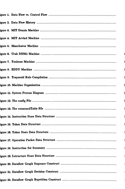
1.1. Data Flow

vs.

Control Flow

One

novel architecture under

study

is

that

of

the

Data Flow

machine.

The data flow

machine

architecture

is based

upon

the

data flow

model of computation.

The data

flow

model

is

not a new

idea, however,

technology

has

only recently

made

it

possible

to

consider computer architectures

based

upon

this

model.

The difference between

the

von

Neuman,

or

"control

flow"

model and

the

data flow

model,

lies in

what controls

the

process of computation within

the

individual

models:

[Miklosko,

Kotov

1984]

Control Flow

(CF)

-

it is

the

_{sequence of}

instructions.

Data Flow

(DF)

-

it

is

the

availability

of

data.

A CF

model program

is

stored

in memory

as a serial sequence of

instructions.

Each

instruc

tion

is

fetched

from

memory

and

then

executed

in

the

processor

(the

von

Neuman

bottleneck).

No

instruction

can execute until all previous

instructions

have

executed.

Thus,

the

processofcomputa

tion

is

controlled

by

the

sequence of

instructions

in

the

program.

This is

the

main obstacle

in

exploiting the

naturalparallelism of algorithms.

In

the

DF

computer,

computation

is

controlled

by

the

flow

of

data

in

the

program.

An

instruction

can execute

only

when all

its

operands are available.

Whether

an

instruction

precedes

another

depends

upon

the

algorithm and not upon

the

location

of

the

instructions

in

memory.

Using

this

method of

computation,

it

is

possible

to

execute as

many

instructions in

parallel as

the

given computer can

simultaneously

handle.

Refer

to

figure

1

for

an

illustration

of

the

difference between

CF

and

DF

computation.

1.2.

Previous

Work

The

originators of research on

data

driven

computing

can not

be

precisely

defined.

In

1968,

Jack

Dennis defined

graphs

to

express algorithms

by

showing

data

dependencies

only;

Tesler

_and

[Ackerman

1982]

CONTROL FLOW

Sequence

of

Instructions

1.P

=

X

+

Y

2.

Q

=

P

/

Y

3. R

= X*

P

4.

S

=

R

-Q

5. T

=

R

*

P

6.RSLT

=

S / T

Computation

Sequence

1

2

3

4

5

6

DATA FLOW

Graph

showing

data

dependencies

X

X

Y

1.P=X

+

Y

3. R

= X*

P

R

,

r

A^

4.

S

=

R

-Q

Computation

Sequence

1

2

and

3

4

and

5

6

=

P/Y

5. T

=

R

*

P

[image:12.529.35.416.219.687.2]

embody

the

syntactic and semantic

features for data flow

programming).

Single

assignment was

developed

by

Klinkhamer

and

Chamberlin in

1971,

and

data flow

graphs were

developed

at

MIT

by

Misunas,

Rumbaugh

and

Kosinski.

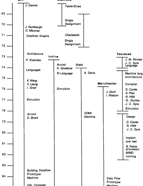
Figure

2

shows some of

the

data

flow

research carriedout since

1968

[Evans

1982].

Following

is

a

survey

of some current

data flow

projects.

1.2.1.

Dennis Machine

at

MIT

Development is

taking

place at

MIT

by

Dennis

and

Misunas.

Project

goals stated

by

Dennis,

Second Data Flow

Workshop

[Misunas

1979]:

1.

Develop

user

level

programming

language.

2.

Build

an

engineering

model.

3.

Address

translation,

optimization,

and code generation.

4.

Develop

specifications

for full-scale

machine.

Current

project status

[Hwang

and

Briggs

1984]:

1.

Prototype

hardware is

under construction.

2.

Compiler is

being

written

for VAL

programming

language.

3.

Fault

tolerance

studies are

being

made.

Figure

3 describes

the

Dennis

machine architecture.

1.2.2.

Arvind Machine

at

MIT

Development

was

begun

at

the

University

of

California,

Irvine

and

is

continuing

at

MIT.

It is

being

directed

by

Arvind

and

Gostelow.

Project

goals stated

by Gostelow,

Second Data Flow

Workshop

[Misunas

1979]:

1.

Design

general-purpose computercomposedof

many

small

processors.

2. Remove bottlenecks

from

the

architecture.

3.

Develop

prototype

based

on

ID

programming

language.

4. Investigate fault

tolerance.

Current

project status

[Hwang,

Briggs 1984]:

1.

ID

programming

language

has been developed.

2.

The

machine

has

not yet

been

built.

MIT

Stanford

69

70

71

72

73

74

75

76

77

78

79

80

81

82

83

84

J. Dennis

Tesler/Enea

J. Rumbaugh

D. Misunas

Dataflow Graphs

Single

Assignment

Architecture

P.

Kosinsky

Languages

HLWeng

C.

Leung

I. Grief

Simulator

Arvind

D. Brock

Chamberlin

Single

Assignment

Irvine

Toulouse

Building

Dataflow

Prototype

Machine

VAL

Compiler

Arvind

K. Gostelow

ID Language

Simulator

Utah

A

Davis

Manchester

DDM1

Machine

J. Gurd

I. Watson

Data Flow

Prototype

Machine

J. M. Nicolas

J. C. Syre

Language

Machine lang.

architecture

Compiler

D. Comte

A. Plas

N. Hifdi

G.. Durrieu

J. C. Syre

Simulator

Design

D. Comte

N. Hifdi

J. C. Syre

[image:14.529.28.499.67.681.2]

Figure

3.

MIT

Dennis Machine

[Misunas

1978]

[Dennis.Boughton,

Leung 1980]

Processing

Section

Processor

Processor

T

/

Control

Network

\

<en control

to

'F

fe.

Distribution

Network

H

F

Instruction Cell

Arbitration

Network

fe

fe,w

Instruction Cell

Memory

Section

Static Execution Rule:

instruction

is

enabled

(can be executed)

if

a

data

token

is

present on

all

its input

arcs and

no

token

is

present on

its

output arcs

Data Token

Control Token

Operation Packet

Memory

Section

Processing

Section

Arbitration

Network

Control

Network

Distribution

Network

-

data

traveling

to the

input

arc

of

an

instruction.

-acknowledge signal

indicating

that

data

has been

removed

from

an

instruction's

output arc.

-

enabled

instruction

and operands

ready

to

be

processed.

-

instruction

cells

_which

hold

instructions

and

their

operands.

-processing

units

that

perform

functional

operations

on

data

tokens.

-

delivers

_operation

packets

from memory

section

to processing

section.

-

delivers

control

tokens

from processing

section

to memory

section.

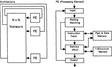
[image:15.529.54.452.90.321.2]

Figure 4 describes

the

Arvind

machine architecture.

1.2.J.

Manchester Machine

Development is

taking

place at

Manchester,

England.

It is

being

directed

by

Gurd, Watson,

and

Kirkham.

Project

goals stated

by Watson,

Second Data Flow

Workshop

[Misunas

1979]:

1.

Major

motivation

is

the

exploitation of parallelism

to

develop

high

speed machine.

2.

Secondary

motivation

is

realization of cost effective and reliable

design.

Current

project status

[Gurd,

Kirkham,

Watson

1985]:

1.

A

data flow

machine

has been

constructed

large

enough

to tackle

realistic applications.

2.

A

small range of

benchmark

programs

has been

written and executed.

3.

Preliminary

evaluationresults are as

follows:

a. a wide

variety

of programs containsufficient

parallelism

to

exhibitspeedup.

b.

a useful

indicator

ofprogramparallelism

has

been

established.

c. aweakness

in

the

present pipeline

implementation

has been

identified

and

fixed.

d.

the

need

for

a separate structurestorage

has been

indicated.

4.

Future

studies:

a.

build

and evaluate a

multi-ring

architecture.

b.

investigate

programs

that

cause match-unit

overflow.

c.

study

low-level

code optimization.

d.

study

data

flow implementation using

VLSI

technology.

e.

improve

machine

to

exceed performanceof

VAX

11/780

mini-computer.

Figure

5 describes

the

Manchester

machine architecture.

1.2.4.

Utah

DDM1 Machine

Development

was

begun

at

Burroughs.

It is

currently

based

at

Utah University.

Davis is

[image:17.529.45.482.73.337.2]

Figure 4. MIT Arvind Machine

[Arvind.Kathail

1981]

[Arvind.Gostelow

1977]

Architecture

NxN

Network

PE

PE

(Processing Element)

PE

Input

T

Waiting

Matching

T

Instruction

Fetch

V

Service

(ALU)

T

Output

Pgm

&

Data

Memory

l-Structure

Memory

T

The Arvind

machine

does

not

follow

the

static execution rule as

does

the

Dennis

Machine (see figure

3).

It instead

allows several

tokens to

be

present on

the

input

and

output arcs

that

lead into

and out

of an

instruction.

In

this way

several

instantiations

of

the

same

instruction

(provided

there

are no

data

constraints)

can execute concurrently.

The

architecture of

the

Arvind

machine

is

said

to

be dynamic.

Input Section

Accepts

tokens

from

either

the

communicationsystem or

the

output section

of

its

same

PE.

Waiting-Matching

Section

Input

tokens

whose

destination activity

requires

two

operands are sent

to

this

section

and are

buffered

until

they

can

be

matched.

When

matched, the

token

set

is

then

sent

to

the instruction-fetch

section.

Instruction-Fetch Section

Combines

an

instruction's

opcode

with

its

operands,

and

sends

the

resulting

operation

packet

to

the

service section.

Service Section

Processes

the

operation

packet;

sends

the

resulting data

token to the

output section.

I-Structure

Memory

Stores

l-structure

tokens.

I-Structures

are an

array-like

data

structure

[Arvind,Thomas1980].

Output Section

[Gurd.Kirkham,

Watson

1985]

[Gurd.Watson

1977]

[Watson.Gurd

1979]

[Watson,

Gurd

1982]

token

packets

J

r

to

h

i

ost

i

Token

Queue

token

packets

I

r

i

Matching

Unit

Overflow

Unit

I/O Switch

i i ii

token-pair

j^

y

packets

Instruction

Store

executa packets

ble

I

Processing

Unit

frorri

nusi

token

p<ackets

The Manchester

machine

is

a

dynamic dataflow

machine,

as

is

the

MIT Arvind

machine

(see

figure

4).

I/O Switch

Token Queue

Matching

Unit

Instruction

Store

Processing

Unit

-

loads

programs and

data

from

host;

permits

results

to

be

output

for

external

inspection.

-smooths out uneven rates of generation and

consumption

of

tokens in

the

ring.

-pairs

together

tokens

destined for

the

same

activity.

-contains

machine code of

dataflow

program.

[image:18.529.59.420.86.360.2]

10

1.

Develop

a recursivemachine architecture.

a. performance gain

is

made as machine

is

physically

extended.

b.

no need

for

electronic

tuning

as

hardware

modules are added.

2.

Develop

a

high-level data-driven

graphical

language

[Davis,

Lowder

1981].

Current

project status

[Treleaven,

Brownbridge

,Hopkins

1982]:

1.

DDM1 became

operational

in

1976

(first

in

the

USA).

The DDM1

communicates with a

DEC

20/40.

The DEC

system

is

used

for

compilation,

input,

output,

and performance measurement.

2.

The language is

currently

a statement

description

of a

directed

graph.

An interactive

graphical

programming

language is

under

development.

Figure

6 describes

the

DDM1

machine architecture.

1.2.5.

Toulouse

LAU Machine

Development is

taking

place

in

Toulouse,

France

by

Plas, Comte,

Syre,

Hifdi.

Project

goals

stated

by

Comte,

Second Data

Flow

Workshop

[Misunas

1979]:

1. Project

was

inspired

by

Tesler

and

Enea

paper on

singleassignment.

2.

Design

a single assignment

high level language:

a.

that

is

easy

to

use

by

non-specialists.

b.

that naturally

exploits parallelism

in

algorithms.

c.

that

is

readableand

debuggable.

3.

Develop

a machine architecture

to

suit

the

single

assignment

language.

Current

project status

[Treleaven,

Brownbridge

,Hopkins

1982]:

1.

The

first

of

32

processors

became

operational

in

1979.

2.

The

remaining

processors

have

been

constructed since.

[Davis

1979]

[Davis

1978]

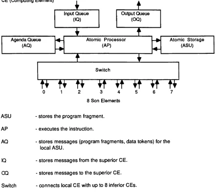
CE

(Computing

Element)

i

?

Input Queue

(IQ)

Output Queue

(CO)

T

t

Agenda Queue

(AQ)

Atomic Processor

(AP)

Atomic Storage

(ASU)

t

1

Switch

0

1

t

n

it

vt

2

3

4

8 Son

Elements

vf

'

5

6

ft

7

ASU

-stores

the

program

fragment.

AP

-executes

the instruction.

AQ

-stores messages

(program

fragments,

data

tokens)

for

the

local ASU.

IQ

-

stores messages

from

the

superior

CE.

CQ

-stores

messages

to

the

superior

CE.

Switch

-

connects

local CE

_with

up to

8

inferior

CEs.

Work in

the

form

of

a

program

fragment is

allocated

to

a

computing

element

by

its

superior

via

the IQ.

If

the

fragment

contains subprograms

and

the

CE

has

sons, then

it

will

decompose

the

fragment

and

allocate

the

subprograms

to

its

inferior

elements.

Otherwise

the

fragment

is

stored

in

the

local

ASU.

[image:20.529.46.488.79.476.2]

Figure

7. Toulouse Machine

[Comte.Hifdi.Syre

1980]

[Syre,Comte,Hifdi

1977]

[Plas.etal

1976]

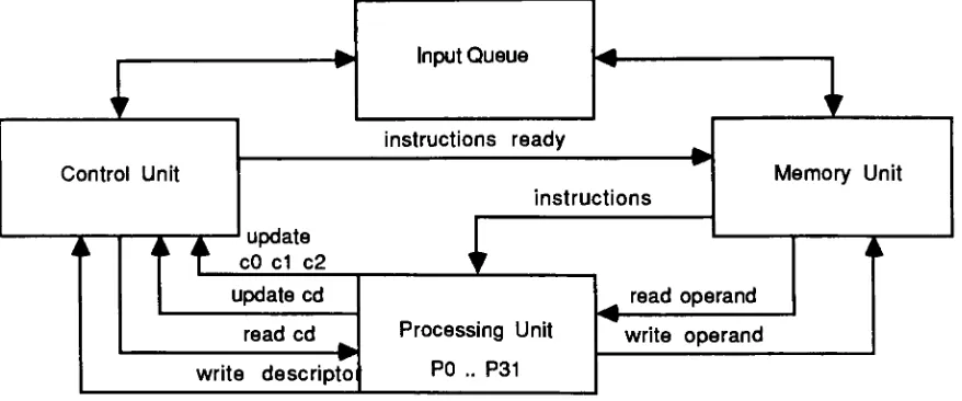
I

Input Queue

1

Control

Unit

instructions

ready

Memory

Unit

update

cO

d

c2

w

instructions

I

t

t

ijpdate cd

1

Processing

Unit

P0

..

P31

read operand

read cd write operand

writ*i

descripto

Memory

Control I

Process

Input Qu

Uni

J

nit

ng

I

eue

[

Jnit

-stores

instructions

and

data.

-maintains

the

control

memory (CO C1 C2).

-consists of

32 identical

processing

elements.

-pool

of work

for the

memory

unit.

The LAU

programming

language is based

on single assignment

rules,

but

the

computer's

program organization

is based

on control

flow

concepts.

In

the computer,

data

is

passed via

sharable

memory

cells

that

are accessed

through

addresses embedded

in instructions.

Separate

control

signals are used

to

enable

instructions.

However,

as

in

data

flow,

the

flow

of

control

is

tied to the

flow

of

data.

Each

instruction

has

three

control

bits

that

denote its

state.

C1

and

C2 define

whether

the

two input

operands are

present.

CO

provides environment control

(for

example,

instructions

within

loops). Cd is

associated

with

each

data

operand and

indicates

if the

operand

is

available.

Two

processors scan

the

control memory:

the

update processor

sets

the

CO C1 C2

bits,

and

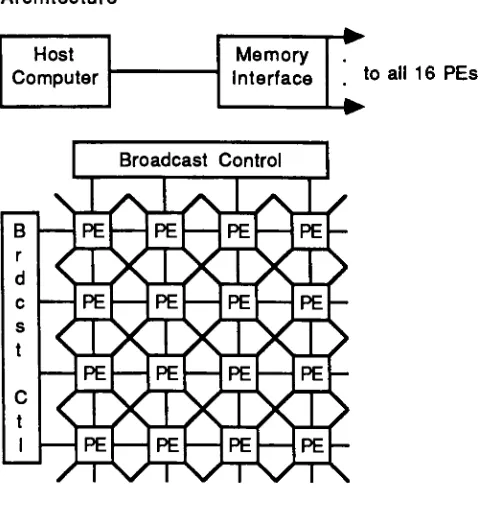
[image:21.529.46.485.74.257.2]

1.2.6.

EDDY Machine

In

Japan,

development

of

the

EDDY

(Experimental

system

for Data-Driven Processor arraY)

is

taking

place.

Current

project status

[Hwang,

Briggs

1984]:

1.

Prototype has been

built.

2.

Compiler for

the

VALID

programming

language has been

developed.

3.

Statistical

data has been

collected:

a. operation rates of

function

units.

b.

average queue

lengths.

4.

This data

will

be

used

to

build

custom

hardware for

the

machine.

Figure

8

describes

the

EDDY

machine architecture.

1.2.7.

Other Projects

As

of

1985

the

only

operational

Data Flow

machinesare

DDM

at

Utah,

EDDY

in

Japan,

the

Manchester

machine

in

the

U.K.,

and

the

French LAU

machine.

Some

other projects of

interest

are

the

Texas

Instruments

Distributed

Data

Processor

[Treleaven,

Brownbridge,

Hopkins

1982].

It

was

built

using

off-the-shelf

technology

and uses a cross

compiler

to translate

FORTRAN 66 into

directed

graph representation.

The Newcastle data-control

flow

computer

integrates data flow

and control

flow

computation

[Treleaven,

Brownbridge,

Hopkins

1982].

Sigmapl in Japan

[Shimada, Hiraki,

Nishida

1984]

will

be built

with

256 processing

elements

[image:23.529.36.275.80.335.2]

Figure 8. EDDY Machine

[Hwang,

Briggs

1984]

Architecture

PE

(Processing

Element)

Host

Computer

Memory

Interface

[-? -?

to

all

16

PEs

Broadcast Control

V-/V-/VYVY

B

PE

PE

PE

PE-r

d

ocXX?

c

PE

PE

PE

PE-s

t

cXXX?

PE

PE

PE

PE-C

t

ocXX?

I

PE

PE

PE

PE

-/nrVurVnrvnr\

Instruc

Mem

Section

Opernd

Mem

Section

Opertn

Unit

Section

Comm

Unit

Section

TT

Broadcast Control

loads

or unloads programs and

data

to

or

from

all

PEs,

in

column or

row,

at

the

same

time.

Instruction

Memory

Section

fetches

an operand

token's instruction

and

sends

both

the

fetched

instruction

and

the

operand

data

to the

Operand

Memory

Section.

Operand

Memory

Section

for

two-operand

operations

the

memory is

searched

associatively for its

partner.

If

found,

the

packet

is

sent

to the

Operation

Unit

Section,

otherwise

it is

stored.

Operation

Unit

Section

executes

the

operation packet and sends

result

tokens

to

the

Communication Unit

Section.

2.

Project Description

This

section

describes

the

data

flow

computer

being

simulated.

Program

representation,

data

representation,

structrure

representation,

machine

organization,

and

the

instruction

set are

detailed

in

this

section.

This

thesis

project

is

an outgrowth of a previous

thesis that

was submitted

to

the

Rochester

Institute

of

Technology.

The

previous

thesis,

"Simulation

of a

Dataflow

Computer", by

Carol

M.

Torsone,

suggests ways

to

improve its

implementation.

Euclid

was used

to

implement

the

original

simulator, thus

limiting

the

use and

testing

of

the

simulator

to

integers.

Torsone

concluded

that

many

"real

life"

applications,

which would

have been

interesting

due

to their

high degree

of

concurrency,

could not

be

programmed

because

of

this

limita

tion.

To

rectify

this,

Modula-2 is

used

to

implement

the

new

simulator,

it

supports

both

integers

and

reals,

and provides coroutines

for

concurrent programming.

The

original simulator

only

allowed

for

single-valued variables

to

be

used as

data

tokens,

which again

limited

the

applications of

the

simulator.

The

new simulator

supports,

in

addition

to

scalar

variables,

I-structures

[Arvind,

Thomas

1980],

which are array-like

data

structures.

The

new simulator

follows

more

closely

the

U-interpreter

algorithm

[Arvind,

Gostelow

1982]

for

tagging

data

tokens,

thus

allowing

nested

loops

to

be

programmed.

Programs

to

be

run on

the

original simulator

had

to

be

written

using

the

simulator's machine

language.

The

new simulator comes equipped with an

assembler,

and

is

programmed

using

an

assembly

language

which

is

astatement representation of

the

dataflow

graph.

Other differences between

the two

simulators

include

the

machine

instruction

format,

the

han

dling

of

constants,

and

the

handling

of

input

andoutput.

Both

projects simulate a

dynamic

dataflow

machine

based

upon

the

machine organization

under

development

at

the

University

of

Manchester

[Gurd, Kirkham,

Watson

1985].

The

machine

16

2.1. Functional

Specification

The

simulator

is based

upon

the

Manchester

machine architecture

[Gurd,

Kirkham,

Watson

1985],

uses

the

token

tagging

scheme of

the

U-interpreter

[Arvind,

Gostelow

1982],

has

an

assembly

language based

on

[Dennis

1975],

and supports

the

I-structure data

structure

[Arvind,

Thomas

1980].

2.1.1.

Program Representation

Dataflow

compilers

translate

high-level

programs

into directed

graphs.

Vertices

in

the

graph

correspond

to

machine

instructions,

and edges correspond

to the

data dependencies

which exist

between

the

instructions.

The implication is

that

instructions

which

depend

on other

instructions

should

be

sequenced

accordingly,

but

where no

dependencies exist,

the

instructions

can

be

executed

in

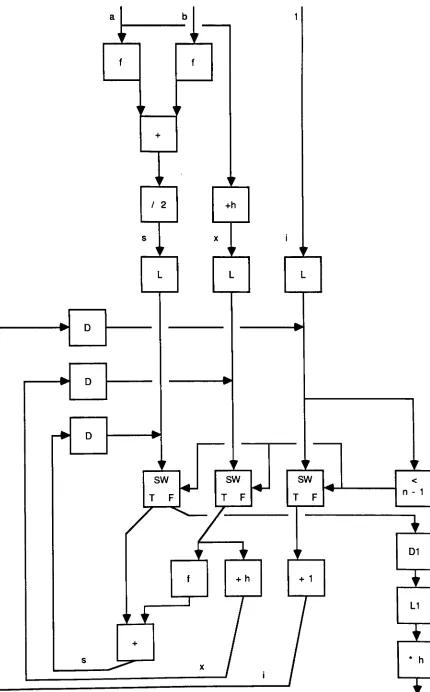
parallel.

A

graphi

cal

translation

is

shown

in

figure

9,

it

was compiled

from

the

following

high-level

program,

which

integrates

a

function

f from

a

to

b

over n

intervals

ofsize

h

by

the trapezoid

rule:

s=(f(a)+f(b))/2

x= _a

+

h

for i

=

1

to

_n-

1

s =_s

+

f(x)

x=_x

+

h

end

for

s =s*h

In figure

9

the

box

marked

f

represents

the

subgraph of

function f.

Instructions

D,

Dl,

L,

and

LI

are

included

to

provide proper

entry,

iteration,

and exit

by

manipulating

context-identifying

information

(discussed in

the

next section).

The

remainder of

the

operators are

arithmetic,

rela

I

l

/

2

+h

SW

T

F

SW

T

F

SW

T

F

1

+

h

<

[image:26.529.74.504.25.717.2]

18

2.1.2. Data Representation

It is

the

processors

's

task to

propagate

data

values

through the

program

graph,

triggering

instructions

when

the

operands are available.

Data

values are carried

by

logical

entities called

tokens.

A

token

contains not

only

a

data

value

but

also

the

address of

its

destination instruction.

Conceptually,

tokens

move about on

the

vertices of

the

graph.

Instructions

axe enabled when

tokens

are present on all

input

edges.

Program

execution consists of an

instruction absorbing its input

tokens,

and

producing

an output

token

for

the

next

instruction in

the

graph.

A

program

terminates

when

there

are no enabled

instructions left.

In

a

dynamic

model,

more

than

one

token

is

allowed

to

be

present on an

arc;

therefore,

the

next-instruction

label

also contains

dynamic,

or context-sensitive

information

(called

the

tag).

These

next-instruction

labels

or

activity

names

[Arvind,

Gostelow

1982]

contain

three

parts:

u:

The

context

field,

which

uniquely

identifies

the

context

in

which

the

instruction is

invoked.

The

context

field is itself

an

activity

name.

i:

The initiation

number,

which

identifies

the

loop

iteration

in

which

this

activity

occurs.

The

field

is

1

outside a

loop.

s:

The

instruction

address.

Since

instructions

may

have

more

than

one

input

operand,

an

index

value,

called

the

port

(p),

which specifies

the

operand number associated with

this

token,

is

also carried on each

token.

The

complete

token

looks like

this:

<u

i

s

data>p

2.1.8.

Structure Representation

Data

structure operations present a problem

for dataflow

machines.

In functional languages

(the

language

of

dataflow),

a

data

structure

is

acted upon as a single

entity;

the

entire

data

struc

ture

moves

through the

program

graph,

and each structure operation results

in

the

creation of a new

because it is

not possible

to

operate on more

than

one structure element at one

time.

[Arvind,

Tho

mas

1980]

propose

the

I-structure

as anew array-like

data

structure,

which can

significantly

reduce

structure

overhead,

and provide

for

highly

parallel structure creation and operation.

I-structure

operations are

based

on

the

premise

that,

in

many circumstances,

full

generality

of

data

structure

operations

is

not

needed;

hence

significant gains should

be

possible

by

substituting

restricted

data

structureoperations.

An I-structure is

an asynchronous structure with a constraint on

its

construction.

I-structure

producerscan

only

append a value once

to

a particular selector of an

I-structure,

no other value can

ever

be

appended

to that

selector

in

that

particular

I-structure.

The

definition

of

I-structure

pro

ducers

permits

individual

appends

to

be done

out of

order,

thus

allowing

concurrent construction of

an

I-structure.

Because I-structures

are

asynchronous,

values can

be

selected

from

an

I-structure

before

the

I-structure is

complete.

The

read-before-write problem

is

handled

by

deferring

allread

requests of an

empty

cell until after

the

first

write operation.

2.1.4.

Machine Organiiation

The

organization

is

based

on

the

Manchester

machine architecture.

(See

figure

10).

2.1.5.

Instruction

Set

The

instruction

set

is

taken

largely

from

[Dennis

1975]

in

which

he defines

a

data

flow

program

as a

bipartite directed

graph where

the two types

ofnodes are called

links

and actors.

He

regards

the

arcs of a

data

flow

program as channels

through

which

tokens

flow carrying

values

from

each

actor

to

other actors

by

way

of

the

links.

The instruction

set proposed

here differs from

[Dennis

1975],

in

that

data is

permitted

to travel

directly

from

one actor

to

another actor.

Links

are used

only to

replicate

tokens

with multiple

destinations.

The

thesis

instruction

set also

includes

actors

necessary

for

implementing

the

U-Interpreter

[Arvind,

Gostelow

1982],

and

for

implementing

Figure

10. Machine

Organization

INPUT TOKENS

DATA TOKENS

I

"

OUTPUT TOKFN5

MATCHING

UNIT

1

TOKEN SETS

DFPGM

UNIT

DF

PGM

INSTRUCTION

UNIT

i i

i

1

OPERATION PACKETS

Dl IT

PROCESSING

UNIT

I-STRUCTURE

STORE

TOKENS

RESULT TOKEIMS

OUTPUT TOKENS

10 Unit

Assembles

program

and

loads

machine

instructions into

the

instruction

store.

Sends input

tokens to

matching

unit.

Sends

output

tokens

to

output

device.

Matching

Unit

Forms

token

set

based

on

activity

name.

Sends

token

set

to instruction

unit

Instruction Unit

Forms

operation

packet

from

machine

instruction

opcode and

token

set.

Sends

operation

packet

to processing

unit.

Processing

Unit

Sends

incoming

operation

packet

to

an

available processor.

Executes

operation

packet.

Sends

result

token

to the matching

unit.

Sends

output

token

to the

10

unit.

-Structure

Store

[image:29.529.44.492.59.351.2]

LINK:

replicates

its

input

token

and

distributes

the

copies

to

its

output

destinations.

LK

-T

+

i

OPERATOR

ACTOR:

applies

its

function

to

its

two

input

tokens

(one,

input

token

for

unary

functions)

and sends

the

result

to

its

output

destination.

T* *T"

f negation, sqrt. abs. -<-, -, /,

DECIDER

ACTOR:

applies

its

predicate

to

its

input

tokens

and sends

the

resulting

control

token

(true

or

false)

to

its

output

destination.

T* *T'

22

BOOLEAN

ACTOR:

applies

its

boolean

function

to

its

input

tokens

and sends

the

resulting

control

token

(true

or

false)

to

its

output

destination.

*t* *t*

b - _{and, or,} not

-T-T-GATE CONTROL ACTOR:

passes

its input

token

to

its

output

destination if it

receives

the

value

true

at

its

control

operand;

the

data

operand

is discarded if false is

received.

-tru -false

F-GATE

CONTROL

ACTOR:

passes

its

input

token

to

its

output

destination

if

false

is

received,

discards

its

input

if

true

is

received.

SWITCH

CONTROL

ACTOR:

allows a control value

to

determine

which of

two

output

destinations

its

input

should

be

passed

to.

A

true

control value will cause

the

input

data

to

be

routed

to

the

T-destination;

a

false

value will cause

the

data

to

be

routed

to

the

F-destination.

T F T F T F

LOOP

ACTORS

(L, LI, D,

Dl):

manipulate

context-sensitive

information

in

the

token

tag,

making it

possible

to

concurrently

execute several

iterations

of a

loop.

The

L

actor adds new contexts

to

the

token

tag

when

loops

are

entered;

LI

removes

contexts added

by

L

when

loops

are exited.

The D

actor adds

1

to

the

initiation

value;

Dl

resets

the

initiation

value

to

1.

while

(p(x))

x =

f(x)

end while

L

D

?

Initial Token

|

x

|

->

|

1

s

|

x =

data

1

=

iteration

s=

sending

_address

Add

new context

to

tag

|

x

|

->

|

1

c

|

->

|

1

s

|

c=_code

block

Increment initiation

value

1

:

|

x

|

->

|

2

c

|

->

|

1

8

|

n :

|

x

|

->

|

n+1 c

|

->

|

1

s

|

Reset initiation

value

I

x

|

->

|

1

c

|

->

|

1

s

|

Remove

context added

by

L

24

APPLY ACTORS

(A, PBEG, PEND,

Al):

operate on context-sensitive

information

in

the

token

tag,

making

it

possible

to

concurrently

execute several

instantiations

of a procedure.

The A instruction

adds a new context

to

the

token

tag

each

time

a procedure

is

invoked,

sends

its input

tokens

(procedure

arguments)

to

the

PBEG

instruction,

and sends

the

Al

instruction

address

(return

address)

to

the

PBEG

instruction.

The

PBEG

instruction

is

always

the

first

instruction

of a

procedure,

it

collects

the

procedure arguments and

distributes

them

to

the

statements of

the

procedure,

and sends

the

Al

address

(return

address)

to

the

PEND

instruction.

The

PEND

instruction

is

always

the

last

instrruction

of a

procedure,

it

collects

the

procedure result

tokens

and sends

them

to

the

Al

instruction.

The

Al

instruction

removes

the

context added

by

A

and

distributes

the

tokens

to

the

statements of

the

calling

procedure.

args args +

A1

a

I

I

A

PBEG

I

args

A1

address

I-STRUCTURE

ACTORS

(IREAD,

IWRITE):

manipulate

I-structures.

xO

i

The IREAD

operation retrieves

the

data

value of

I-structure

xO at selector

i.

xO

i

Ui

IWRITE

The IWRITE

operationappends

the

value v

to

I-structure

xO at selector

i.

It

also satisfies

26

S.

Project Implementation

This

section

discusses

the

simulator

implementation.

It describes

the

inputs,

outputs, data

structures,

and algorithms of

the

processes

that

constitute

the

system.

It

endswith a

discussion

of

the

monitors andprocess synchronization used

to

simulate parallelexecution.

The

simulator was written

in ModuLv2.

ModuLv2

was chosen

because

it

supports real

numbers and provides coroutinesas avehicle

for

simulating

concurrentexecution.

The

simulator will support a maximum of

five hundred instructions

per

program,

twenty

argu

ments per subroutine

call,

and one

hundred i-structures

of

fifty

cells apiece.

Any

of

these

limits

may

be

changed

by

modifying

the

DataFlowDecls.def file

and

recompiling

the

simulator.

The

current

limits

were chosen

to

achieve reasonable run-time performance.

The

simulator operates

only

on numerical

data

(with

the

exception of output

labels).

Data

may

be

entered as either

integer

or

real; the

simulator converts all values

to

real numbers.

Control

values are represented

by

a

1

for

true

and a

0

for false.

The

simulator consists of

five

functionally

different

processes

(see

figure 11).

Build

token

set

simulates

the

match

unit,

build

operation packet simulates

the

instruction

unit,

execute operation

packet simulates

the processor,

and

the

remaining

processes simulate

the

10

unit.

The

simulator

begins

by

executing

the

assemble

instruction

process

to

convert

the

dataflow

assembler program

into

the

simulator's machine code.

The

read

data

process reads

the

input file

and produces

input

tokens.

The

config

file

(see figure

12)

is

read

to

determine

the

number of proces

sors

that

are

to

be

activated

for

this

invocation;

a separate execute operation packet coroutine

is

started

for

each active processor.

Build

token

set and

build

operation packet are started as corou

tines

to

simulate

the

matchunit and

instruction unit,

respectively.

Execution begins

when

the

read

data

process produces

input

tokens.

Execution

of

the

simula

tor

precedes as

the

token,

token set,

andoperation packet queues are produced and consumed.

Exe

Assembler

Program

Instruction

Store

Token Set

Queue

Operation Packet

Queue

Token

Store

Token

Queue

[image:36.529.51.487.78.702.2]

28

Figure

12.

The config file

20

2000000

2000000

2000000

20

is

the

number of processors

to

be

activated.

2000000

is

the

working

set size of

the

match unit coroutine.

2000000

is

the

working

set size of

the

instruction

unit coroutine.

2000000

is

the

working

set size of

the

processor coroutines.

The

config

file

may

be

edited prior

to

running

the

simulator

to

establish

the

number of

processors

that

are

to

be

activated

during

the

simulation.

3.1.

Assemble

Instruction

Process

The

assemble

instruction

process reads

the

file

containing

the

dataflow

assembler

commands,

assembles

the

commands

into

the

simulator machine

code,

and

stores

the

machine code

in

the

instruction

store

data

structure.

The

assemble

instruction

process also stores each

instruction's

enable and constant counts

in

the

token

store.

The

simulator

instruction

format

is

as

follows:

OP

EC DC CC

20{PORT}20 20{DEST}20

OP

EC DC CC

LABEL

20{PORT}

20{DEST}20

(OUTPUT

and

DEBUG

instructions)

OP

Instruction

opcode.

EC

Instruction

enable count.

This

is

the

number of operands needed

to

execute

the

instruction.

DC

Instruction

destination

count.

CC

Instruction

constant count.

PORT Slots in

the

instruction

where

incoming

operands are stored.

These

slots

include

a constant presence

bit.

The CONST

assembler

directive

stores

the

constant value

in

the

port,

sets

the

constant presence

bit,

and

increments

the

constantcount

by

one.

There

are

twenty

slots per

instruction.

DEST Destination

address and port.

These

are

the

instruction

addresses and ports

where

the

result

tokens

(produced

by

executing

the

instruction)

are

to

be delivered.

There

are

twenty

of

these

per

instruction.

The

assemble

instruction

process

begins

by loading

the

command

table.

The

commandTable

file

contains

the

syntactical

information

needed

to

assemble

the

simulator's

dataflow

programs.

The

table

has for

each assembler

instruction,

the

instruction's

mneumonic, opcode,

enable

count,

and

destination

count

(see figure

13).

The

instruction

store

is

an

array

of

five hundred instruction

store records

(see

figure

14)

.

An

instruction's

address

is

its index

value

into

the

array.

The

zero

instruction

address

has

a special

meaning

for

the

assembler;

it is

reserved

for

specifying

a null

destination

address.

3.2.

Read Data

Process

The

read

data

process reads

the

input

file,

builds

an

input

token

from

each record

in

the

file,

and sends

the

input

tokens

to the token

queue.

This

is

the

process which puts

the

simulator

in

motion.

The input file

record consists of a

data

value and a

destination

(recall

that

a

destination

con

sists of an

instruction

address and a port number).

The input

file is further discussed in

the

Project

Application

section.

3.2.1.

Token

Implementation

Tokens

consist of a

data

value

(data

values are not

distinguished from

control

values),

an [image:38.529.110.352.64.228.2]

30

Figure

13.

The

commandTable

file

#

100

0

0

A

1

0

1

Al

2

0

0

ABS

31

1

ADD

3

2

AND

4

2

CONST

101

0

D

5

1

Dl

6

1

DEBUG

34

0

DIV

7

2

EQ

8

2

FGATE

9

2

GE

10

2

GT

11

2

HALT

32

1

IFREE

33

3

IREAD

12

2

IWRITE

13

3

L

14

2

LI

15

1

LE

16

2

LINK

17

1

LT

18

2

MUL

20

2

NE

21

2

NEG

22

1

NOT

23

1

OR

24

2

OUTPUT

19

0

PBEG

25

0

0

PEND

26

0

SQRT

27

1

SUB

28

2

SWITCH

29

2

2

TGATE

30

2

1

TRACE

102

0

0

Column

1

contains

the

instruction

mneumonic.

Column

2

contains

the

instruction

opcode.

Column

3

contains

the

instruction

enable count. [image:39.529.54.266.119.574.2]

Figure

14.

Instruction

Store

Data

Structure

1

OP

EC DC CC L

Px

.

P20D1-D20

500

OP

EC DC CC L

Px

.

P20D1

D20

OP

instruction

opcode.

EC

instruction

enable count

(number

of operands needed

to

execute

instruction).

DC instruction

destination

count.

CC

instruction

constant count.

L

character

string

that

labels

output

data.

P

slots

for

receiving

instruction

operands.

D

destination

address and port where

the

instructions's

result

tokens

are

to

be

sent.

information

(see

figure

15).

3.3.

Build

Token

Set

Process

The

build

token set process

forms

tokens

into

sets which are

destined

for

the

same

instruction

and

have

the

same context.

A

token set

is

complete when all

the

tokens

needed

to

enable an

instruction

are gathered

together.

Completed

token

sets are

sent

to

the

token set queue.

Tokens

which

by

themselves enable an

instruction,

and

tokens

which when

combined with an

instructions's

constants enable an

instruction,

are made

into

a

token

set of one and queued.

The

token

matching

algorithm searches

the

token store

(see

figure

16)

for any

token sets whose

destination

is

that

of

the

token.

If

a

matching

set

is found

then

the

[image:40.529.65.475.108.417.2]

32

Figure

15.

Token Data Structure

Activity

Name

(Tag)

LIFO

queue

Destination

Context

data

na >

i

s >

i

s/c >

i

s/c

data

data

value or control value.

na number of

activity

names

in

the

tag.

i

initiation

number

(loop

iteration

counter).

s

instruction

address and port.

c

loop

code

block

number.

s/c

indicates

that

in

some

instances

the

address

is

part of

the

activity

name,

while other

times

it is

the

code

block

number.

When loops

are entered

it is

the

loop

code

block

number

that

is

needed

to

match

tokens.

When

subprograms are

invoked it is

the

invoking

instruction's

address

(the

A

instruction)

that

is

needed

to

match

tokens.

na

is

used

to

improve

the

simulator's run-time execution speed.

It

speeds

up

the

token

matching

algorithm

by

allowing

it

to

immediately

discard

tokens

whose

activity

name counts are

unequal;

this

eliminates needless

traversing

of

activity

name queues when

matching

token

activity

names.

the

appropriate

token

set

port,

and

the

token

set count

is

incremented.

If

the

instruction

enable count equals

the

token

set count

then

the

set

is

queued and

deleted

from

the

token

store.

If

a token

is

the

first

in

its

set

to

arrive,

a

token

set record

is

created and

inserted

into

the token store at

the

end of

the

queue

for

that

token's

destination

address.

The

token

data

is

inserted

into

the

appropriate

port,

the

token

set

activity

In

the

event where a

token

is

destined

for

an

instruction

that

is

already

occupied,

the

simulator will

issue

an error message and abort execution.

Figure

16.

Token

Store

Data Structure

1

max

instruction

ec cc ec cc

1

1

1

V

1

V

tc

>

p..p

na

1

>|

i

s

|

/ /

>

|

i

s/c

|

Token

Set

Activity

Name

tc

na

->

P-P

Token Set

Ports

I

>|

i

s

|

/ /

>

|

i

s/c

Token

Set

Activity

Name

ec

cc

tc

P

na

i

s

c

instruction

enable count.

instruction

constant count.

number of

tokens

int

the

token set.

port

containing

token

set

values;

a

bit

is

set

to

indicate

data

present.

number of

activity

names

in

the

tag.

loop

iteration

counter.

instruction

address and port. [image:42.529.55.466.176.579.2]

34

3.4.

Build

Operation

Packet

Process

The

build

operation packet process

combines

token

sets with

their

destination

instruction's

opcode,

enable

count,

destination

count,

output

label

(if

there

is

one),

and

constant values

(if

there

are any).

The

completed

packet

is

sent

to

the

operation packet

queue where

it

waits

to

be

executed

by

the

next available processor.

3.5.

Execute

Operation

Packet

Process

The

execute operation packet

invokes

the

appropriate procedure

to

perform

the

operation specified

by

the

operation packet's opcode.

The

data

resulting

from

the

operation,

and

the

operation packet's

destination

and context are

formed

into

a result

token

and sent

to

the

token

queue.

The

simulator

instruction

set

is

completely

defined

in

the

Project

Description

section

(see

section

2.1.5).

Each

instruction

is

implemented

as a separate procedure.

The

instruction

set can

be

easily

extended

by

Figure

17.

Operation

Packet Data

Structure

|

op

ec

dc 1 p..p

d..d

na

|

>

|

i

s

|

/ /

>

|

i

s/c

|

op

instruction

opcode.

ec

instruction

enable count.

dc

instruction

destination

count.

1

output

label.

p

port

containing

operand

value;

a

bit is

set

to

indicate data

present.

d

destination

address and port of result

token.

na number of

activity

names

in

the

tag.

i

loop

iteration

counter.

s

instruction

address and port.

writing the

instruction

procedure and

linking

it

with

the

rest of

the

simulator modules.

Placing

the

instruction's

command syntax

into

the

commandTable

file

(see

figure

13)

will

incorporate

the

instruction

into

the

simulator'sassembler

language.

3.5.1. I-Structure

Implementation

The i-structure

store

(figure

19)

is

an

array

of one-hundred

by fifty

i-structure

cells.

The

i-structure

is implemented

as an asynchronous

(allows

reads

to

occur

before writes) data

structure

that

provides mostof

the

general

functionality

of

data

structures.

It is

constrained