Presentations of the Mapping Class Group

(1)

Presentations of the Mapping Class

Group

Adele Jackson

October 2018

A thesis submitted in partial fulfilment of the requirements for the degree of Bachelor of Philosophy (Honours) in Mathematics

(2)

(3)

Declaration

The work in this thesis is my own except where otherwise stated.

(4)

(5)

Acknowledgements

Firstly, I would like to thank my supervisor, Joan Licata. Thank you for picking such an interesting topic, and for all of your time looking at graphs! It’s been a great year, mathematically and otherwise.

I would also like to thank all of the other researchers who I have learned so much from, especially Vigleik Angelveit, Pierre Portal, Griffith Ware, Jim Borger, Scott Morrison and Ben Burton (UQ). I’ve had the chance to take so many fascinating courses here. I’ve really enjoyed the last four years.

Thanks to everyone who proofread parts of my thesis – Matthew Alger, Chris Williams, Alex Grant and Sufyan Saleem.

Thanks also to my fellow honours students for helping me stay sane, especially Chris, Jane, Kyle, Hugh, Feng and Sam. Thanks also for the copious amounts of jelly and chocolate. Similarly, my housemates Julia, Angus and Tracy have been a great support.

(6)

(7)

Abstract

(8)

(9)

Notation and terminology

We will assume all surfaces are orientable and connected with no punctures, though they may have boundary components. In the following, S is an orientable surface,∂S is its boundary, and x is a point in S. We use g for the genus of a surface, and n for the number of boundary components. A closed surface is one with no boundary components.

All groups of maps from S to S come with the compact-open topology (Defini-tion 2.2), and if F is such a group of maps containing the identity, we take π1(F) to

be based at the identity.

We will identify the following objects, which are defined in Chapters 4-6:

1. an edge eof a marked bordered fatgraph,

2. the graph dual of e, which we can view as an element of the fundamental path groupoid, and

3. if e is in the canonical generating set for the fundamental path groupoid, the image of e under branch reduction. This image is an edge in a chord diagram that has the same dual ase.

Notation

Ifc1 andc2 are oriented chords, we writec1 c2 if the initial point

ofc1 immediately precedes that of c2.

[a, b] The commutator ofaand b,aba−1b−1.

{pi} On Σg,n, this is a collection of nmarkeddual points, disjoint from

thenmarked points, with one on each boundary component. e Ifeis an oriented edge in a graph or chord diagram,eis the same

edge with the opposite orientation.

(12)

π1(S, X, x) The relative fundamental group. Forx∈X⊂S, this is homotopy

classes of maps (D1, S0, s0)→(S, X, x) whereD1 has endpointss0

and s1.

Π1(S,{pi}) Let Π1(S) be the fundamental path groupoid of S, that is, the

groupoid consisting of homotopy classes of paths inS. Then Π1(S,{pi})

is the full subgroupoid of Π1(S) containing all paths that start and

end at points in{p_i}..

Σg,n A fixed orientable genus g surface with n boundary components,

with an ordering on the boundary components. Comes equipped withnmarked points, one on each boundary component.

Dn The n-dimensional closed disk.

Diff(S) The group of diffeomorphismsS →S.

Diff+(S) The group of orientation-preserving diffeomorphismsS →S. Diff(S, ∂S) The group of diffeomorphismsS → S that fix the boundary ofS,

∂S, pointwise.

Diff(S, ∂S, x) The group of self-diffeomorphisms of S that fix∂S pointwise and sendx to itself.

Diff(SrelX) The group of self-diffeomorphisms of S that fix X⊂S as a set. Homeo(S) The group of orientation-preserving homeomorphismsS →S. This

can be modified in the same way as the group of diffeomorphisms (for example, Homeo(S, ∂S)).

M od(S) The mapping class group of S. This is the group of orientation-preserving homeomorphisms (or diffeomorphisms) of our surface S, that fix∂S pointwise, up to isotopy also fixing ∂S. See Defini-tion 2.3.

Pn The pure braid group on nstrands. See Definition 2.15.

P(X;n) Configuration space ofnpoints inX. See Definition 2.14. Sn The n-dimensional sphere.

(13)

Tγ A Dehn twist aboutγ.

T(e) For ean edge in the maximal tree of a bordered fatgraph, this is the subset of the maximal tree that is disconnected from the tail within the tree if we remove e.

(14)

(15)

Chapter 1

Introduction

The mapping class group M od(S) is the group of isotopy classes of homeomorphisms from a surface to itself. It is an important algebraic invariant of a surface, and is deeply connected to Teichm¨uller space and the moduli space of Riemann surfaces homeomor-phic to S. One natural problem is to find a “nice” presentation of the mapping class group. Such a presentation allows us to easily work with and investigate the group.

We first consider a presentation developed by Hatcher and Thurston. Its generators are Dehn twists (Definition 2.5), which are a type of mapping class that arises naturally in the 2-manifold context. A classical result of Dehn and Lickorish shows thatM od(S) is finitely generated by Dehn twists [Lic64]. More recently, Hatcher and Thurston showed that for a certain choice of Dehn twist generators ofM od(S) for closed surfaces S, one could construct a finite generating set of relations [HT80].

After giving some background in Chapter 2, in Chapter 3 we give an exposition of this Dehn twist presentation of M od(S). Hatcher and Thurston show that one can construct a finite presentation whose generating set is Dehn twists, but leave an explicit execution of it to the reader. They examine the action ofM od(S) on a certain combinatorial complex, the cut system complex (Definition 3.2). They prove that a series of fibrations of diffeomorphism spaces determines a presentation of the subgroup ofM od(S) that fixes a vertex of this complex, then build the full presentation from this. While Wajnryb gave a very explicit exposition of their work, his intentional choice of elementary techniques mean his approach is substantially removed from the fibrations and exact sequences of homotopy groups used in the original paper [Waj99]. Chapter 3 bridges this gap in techniques, using Hatcher and Thurston’s fibrations and the Birman exact sequence (Theorem 2.22). We derive an explicit presentation of the subgroup of M od(S) that fixes a vertex for genus one and two surfaces, then discuss how to extend this to a presentation of the whole group.

(16)

different contexts other generators arise. Penner, among others, considers cell decom-positions of Teichm¨uller space that have an action of M od(S) [Pen87; Pen04]. In this setting, the edges of this cell complex provide a natural set of generators. One cell de-composition of Teichm¨uller space has graphs embedded inSas vertices (Definition 5.4) and Whitehead moves on these graphs as edges (Definition 5.3). We naturally have a presentation of the fundamental path groupoid whose generators are the Whitehead moves, and whose relations are the faces in the complex. The Whitehead move pre-sentation has a much more combinatorial flavour than Hatcher and Thurston’s more algebraic topology-influenced work.

As in Hatcher and Thurston’s presentation, the action of M od(S) on the complex can be used to find a presentation of the group. In this case, the result is an infinite presentation of M od(S) whose generators are Whitehead moves. For surfaces with one boundary component, Bene showed that this Whitehead move presentation of the fundamental path groupoid of the complex can be translated to one whose generators are chord slides [Ben10] using the branch reduction algorithm [ABP09]. This chord slide presentation of the fundamental path groupoid is finite, and by restriction gives an infinite presentation of M od(S). Bene builds on work lifting various representa-tions ofM od(S) to fundamental path groupoids in combinatorial complexes, which has been particularly successful in the connected boundary case (for example, see [ABP09] and [MP08]).

A chord slide presentation ofM od(S) has applications in bordered Heegaard Floer homology, which is an invariant of a three-manifold with boundary that generalises the Heegaard Floer invariants for closed 3-manifolds. Heegaard Floer homology has been one of the most important developments in low-dimensional topology this century. It gives rich and complicated new structures, and has been instrumental in proofs of previously open problems, such as computing knot genus. The fundamental Heegaard Floer invariant for a closed three-manifoldY isHFd(Y). The bordered theory computes

d

HF(Y) as an iterated Hom space of modules associated to a standard handlebody and a set of generators ofM od(S). In the Heegaard Floer context, the morphisms associated to the chord slide generators of M od(S) are called arc slides, and these have been computed for the surfaces covered by Bene’s work.

In Chapters 4-6, we extend Bene’s chord slide presentation from surfaces with one boundary component to those withnboundary components for anyn≥1. The results in these chapters have potential applications in low-dimensional topology. As noted in Section 1.6 of [LOT14], the current bordered Heegaard Floer techniques can be used to computeCFd(Y) for a 3-manifold presented as an open book with a connected binding.

(17)

functions on a surface. A presentation of Mod(S) in terms of these generators would be a significant step towards a classification of the Morse structures compatible with a fixed contact structure.

Our extension of Bene’s work proceeds as follows. First, in Chapter 4, we define a marked bordered fatgraph as in [God07] and discuss its dual, a quasi-triangulation, to show that the mapping class group acts freely on the set of marked bordered fat-graphs. In Chapter 5, we define the marked bordered fatgraph complex, which is homotopy equivalent to Teichm¨uller space [God07; Har86]. The action of the mapping class group on this complex gives an infinite presentation of M od(S) whose generators are Whitehead moves (Corollary 5.12). In Chapter 6, we generalise Bene’s chord slide presentation by extending the branch reduction algorithm [ABP09] to thenboundary component context. The branch reduction algorithm takes a fatgraph to a chord dia-gram, which we show is determined by a canonical set of generators of the fundamental path groupoid of the surface that is associated to the marking of a fatgraph. We show that, under this algorithm, the images of Whitehead moves on fatgraphs are generated by chord slides (Theorem 6.20). We find a set of chord slide generators for M od(S) for surfaces with boundary, and show one can construct a finite but large relation set. We give a simpler candidate relation set (Conjecture A). The proof that the relations in Conjecture A generate all relations is not complete, as we have not checked all the necessary cases.

The marked bordered fatgraphs defined in Chapter 4 have been previously explored, and Sections 4.1 and 4.2 are an exposition of previous work. Section 4.3, which dis-cusses the dual of a marked bordered fatgraph, is a topological approach to Harer’s arc-system [Har86] and Penner’s quasi-triangulation [Pen04]. The marked bordered fatgraph complex (Section 5.1) is well-known, and by taking the dual of its vertices is homeomorphic to Harer’s arc-system complex. For example, this complex can be used to compute the homology of the mapping class group for punctured or bordered surfaces [God07]. However, to the author’s knowledge, marked bordered fatgraphs have not been applied to find a presentation of the mapping class group aside from in the connected boundary case.

(18)

(19)

Chapter 2

Background

In this chapter we introduce the mapping class group of a surface and provide some background material for the rest of this thesis. See [FM12] for more details.

LetSbe an orientable genusgsurface withnboundary components. It is a conven-tion of a field to say thatS is aclosed surface if it has no boundary components. Let Homeo(S, ∂S) be the group of boundary-fixing orientation-preserving homeomorphisms of S, and Diff+(S, ∂S) be the boundary-fixing orientation-preserving diffeomorphisms of S.

2.1 Some results on the mapping class group

First, we define the fundamental group and fundamental path groupoid.

Definition 2.1. Let S be a topological space. Thefundamental group of S based at x∈S,π1(S, x), is the group of homotopy classes of paths that begin and end at xwith

composition.

Thefundamental (path) groupoidofS, Π1(S), is the groupoid of homotopy classes of

paths inS, which may begin and end anywhere inS. There is a composition operation on pairs of pathsf, g such that f ends at somex∈S and g starts atx.

By convention, the composition of pathsf gis the mapI →Sthat sendst∈[0,1/2] tof(2t) and t∈[1/2,1] tog(2t−1).

Note that in the fundamental group, the identity is the trivial path I → {x} and the inverse of a path is the same path with the other orientation. See [Hat01, Chapter 1] for a verification of these claims. There is a natural inclusion of the fundamental group in the fundamental groupoid.

We define a topology on a space of maps S →S.

(20)

compact-2.1. SOME RESULTS ON THE MAPPING CLASS GROUP

open topology onF is generated by

VU,K={f ∈F|f(K)⊆U}

forU ⊂S open andK ⊂S compact.

When we write Diff(S), or any other space of maps of a surface, we will assume it has the compact-open topology. This will allow us to consider the homotopy groups of the spaces of diffeomorphisms or homeomorphisms. With this topology, as our surfaces are Hausdorff and compact, the connected components of Homeo(S, ∂S) are isotopy classes of homeomorphisms, and paths are isotopies. We will take as a convention that π1(Homeo(S, ∂S)) is based at the identity.

Definition 2.3. The mapping class group M od(S) of S is the group of (boundary-fixing) isotopy classes of Homeo+(S, ∂S).

Note that the set of isotopy classes ofHomeo(S, ∂S) is preciselyπ0(Homeo(S, ∂S)).

This definition is equivalent to several others.

Theorem 2.4 (Theorem 6.4 [Eps66], [Bae27], [Bae28], Theorem 6.3 [Mun60]). The following groups are isomorphic:

M od(S) =π0(Homeo(S, ∂S))

∼

= Homeo(S, ∂S)/homotopy ∼

=π0(Diff+(S, ∂S))

∼

= Diff+(S, ∂S)/smooth isotopy.

We call an element ofM od(S) amapping class. Note that a mapping class acts on the set of simple closed curves and on the fundamental group(oid).

Some particularly important mapping classes are the Dehn twists.

Definition 2.5. Let α be a simple closed curve in S. The Dehn twist about α,Tα, is

defined as follows.

LetA=S1×I be the annulus, with orientation from some embedding in the plane. Let the twist about A,T :A→A, be the map sending (θ, t)7→(θ+ 2πt, t). Note that T is orientation-preserving and fixes the boundary of the annulus pointwise.

LetU be a neighbourhood of α, with ϕ:U →A an orientation-preserving homeo-morphism. Then Tα acts as follows:

Tα(x) =







x x6∈N

(21)

2.1. SOME RESULTS ON THE MAPPING CLASS GROUP

(a) Before the Dehn twist. We will twist aroundαin the neighbourhood U.

(b) The resulting curve after the Dehn twist.

Figure 2.1: The effect of a Dehn twist onα on the purple curve.

For example, see Figure 2.1.

We give some basic results on Dehn twists. Let a and b be homotopy classes of simple closed curves with representatives α and β respectively. Let i(a, b) be the algebraic intersection number ofa and b. This is the minimal number of intersections between any two representatives ofaand b.

Now, Tα acts on β as follows. Replace each piece of β that crosses α by a piece

that turns left as it approachesα, does one circuit ofα, and then turns right to follow β again.

We give some special cases for Ta and Tb depending on the intersection number of

aand b.

Lemma 2.6. If α and β are simple closed curves of homotopy classes aand b respec-tively, with i(a, b) = 0, then Tα acts trivially on β.

Proposition 2.7 (Braid relation, Prop. 3.11 [FM12]). If i(a, b) = 1, then TaTbTa=TbTaTb.

It is a classical result that the Dehn twists generate the mapping class group, and that in fact one can pick a finite generating set.

Theorem 2.8 (Dehn (1938), Lickorish (1964), [Lic64]). If S has no boundary compo-nents, M od(S) is generated by finitely many Dehn twists about non-separating simple closed curves.

(22)

2.2. ADDITIONAL USEFUL RESULTS

2.2 Additional useful results

We give some results we will reference in later chapters. Isotopies of curves inS can be extended to isotopies ofS.

Lemma 2.10 (Proposition 1.11, [FM12]). Let F :S1×I →S be a smooth isotopy of simple closed curves. Then there is an (ambient) isotopy Fe :S×I →S such that for

x∈S, F(xe ×0) =x, and for y=F(θ,0), Fe(y, t) =F(θ, t).

By observing that the mapping class group of the disk is trivial, we have the fol-lowing lemma.

Lemma 2.11 (Alexander Trick). Let f : D2 → D2 be a map fixing the boundary pointwise. Thenf is isotopic to the identity by an isotopy fixing the boundary pointwise. We can describe diffeomorphism classes of a disjoint union of circles as a permutation group.

Definition 2.12. The signed permutation group on g elements, ±Symg, is the group

of permutations σ of {±1, . . . ,±g}such that σ(−k) =−σ(k).

Lemma 2.13. The smooth isotopy classes of diffeomorphisms of circles,π0 Diff Sni=1S1

, is isomorphic to ±Symn.

Proof. Letαn be the nth copy ofS1. Define a homomorphism

φ:π0 Diff g

[

i=1

S1

!!

→ ±Sym_g

as follows. For [f] an isotopy class of diffeomorphisms with a representative f and n >0, let|φ([f])(n)|be the integer such that f(αn) =α|φ([f])(n)|. This is well-defined, as, since f is a diffeomorphism, it sends αn surjectively to exactly one αj. Further, f

is injective, so forn6=m,|φ([f])(n)| 6=|φ([f])(m)|. Now, consider f|_α_n. This is a map S1_→ _S1_{, so}_f_|

αn is isotopic to ωk, the winding number kmap. As it is a diffeomorphism, it is injective, so is isotopic to ω±1. Let the

sign of φ([f])(n) be + iff|_α_n is isotopic toω1, and− iff|αn is isotopic toω−1. Thenφ is an isomorphism.

The braid group appears naturally as the fundamental group of configuration space. We briefly discuss this space. For more details, see Chapter 9, [FM12], particularly Section 9.3.

LetD(S×n_{) be the points in}_S×n _{where at least two coordinates are equal.}

(23)

2.3. BIRMAN EXACT SEQUENCE

Definition 2.15. Letφbe a homomorphism from the braid group onnstrands,Bn, to

the symmetric group on nelements,Symn, that acts as follows. Forb∈Bn,b induces

a permutation on then strands. Letφ(b) be this permutation. The pure braid group on nstrands, Pn, is the kernel of φ.

Equivalently, the pure braid group is the subgroup of Bn that induces the trivial

permutation on the strands.

Lemma 2.16 (p.249 [FM12]). The pure braid groupPn is isomorphic to π1(P(D2;n))

where D2 is the disk.

This theorem is a consequence of a generalised version of the Birman exact sequence (Theorem 2.22) from one marked point tonmarked points. We describe the pure braid group in terms of generators and relations.

Proposition 2.17 (Theorem 16, [Art47]). The braid group on n strands has a finite presentation with generators σi for 1 ≤i < n, which takes strand i over strand i+ 1,

and relations σiσj =σjσi if |i−j|>1, and σiσi+1σi =σi+1σiσi+1 for 1≤i < n−1.

Proposition 2.18 (p. 251 [FM12], Theorem 18 [Art47]). The pure braid group Pnhas

the following presentation.

For 1≤i < j ≤n, let Ai,j = (σj−1· · ·σi+1)σ2i(σj−1· · ·σi+1)−1.

Then Pn is generated by all such Ai,j, with relations, for all 1≤i < j < k < l≤n,

as follows:

[Ai,j, Ak,l] = 1 j < k

[Ai,l, Aj,k] = 1 i < j < k < l

[Ak,lAi,kA−_k,l1, Aj,l] = 1 i < j < k < l

and the relation that the three cyclic permutations of Ai,kAj,kAi,j are equal.

2.3 Birman exact sequence

The Birman exact sequence relates the mapping class group of a surface to the mapping class group of the same surface with a fixed point. The exactness of this sequence is proven in Theorem 4.6, [FM12], but the authors only outline the main steps of the proof. For example, they do not explicitly show the maps in the sequence are P ush and F orget.

Let S be a surface with x ∈ S. This theorem will give us a well-defined map P ush:π1(S, x)→M od(S, x), which we will use in Chapter 3.

(24)

The mapping class group ofSwith a fixed pointx,M od(S, x), is Homeo+(S, x, ∂S)/∼ where for f, g∈Homeo+(S, x, ∂S),f ∼g if there is some isotopy fixingx from f tog.

We first give a lemma on the centre ofπ1(S).

Lemma 2.20. Let S be a compact surface with χ(S)<0. Then π1(S) is centreless.

Proof. (This proof follows ideas from Keeley Hoek and Chris Hone.)

Asχ(S)<0, we have 2g+b >2 wheregis the genus andbthe number of boundary components of S.

Ifb >0, the surface S deformation retracts to a wedge sum of circles. The funda-mental group is thus free, so trivially centreless.

Otherwise, supposeb= 0 sog >1. Then

π1(S)∼={a1, b1, . . . , ag, bg|a1b1a−11b

−1 1 · · ·a

−1 g b−g1}.

Consider the quotient π1(S)/hb1, . . . , bgi. This is {a1, . . . , ag|a1a−11· · ·aga−g1}. Note

thata1a−11· · ·agag−1= 1 trivially, soπ1(S)/hb1, . . . , bgiis the free group onggenerators,

for g > 1, so is centreless. Also, the kernel of this quotient map is similarly the free group on{b1, . . . , bg} which is also centreless.

Suppose x ∈ π1(S) such that x commutes with all elements of π1(S). We must

have x7→ 1 in π1(S)/hb1, . . . , bgi, as this group has trivial centre. Thus x must be in

the centre of the kernel, which is trivial. Therefore x is trivial, so π1(S) has trivial

centre.

Before proving the Birman exact sequence, we will define the maps in it. The map F orget :M od(S, x) →M od(S) acts by inclusion. The equivalence class of an element of M od(S, x) up to isotopy not fixingx is an element ofM od(S).

Definition 2.21. The mapP ush:π1(S, x)→M od(S, x) is defined as follows.

Letα :I → S be a representative of an element of π1(S, x). We can view α as an

isotopy of points {∗} ×I →S. We can consider α−1 as an isotopy of curves by I×I −−−−−−→ {∗} ×projection I α

−1 −−→S.

We can extend this to an isotopy of the whole surface S, F : S ×I → S, such that F|S×0 is the identity onS (Lemma 2.10). Let φ be the homeomorphism at the end of

this ambient isotopy, that is, F(−,1). Then P ush(α) is the equivalence class of φ in M od(S, x).

(We use α−1 _{here as by convention composition in} _π

1 is left to right, but in M od

(25)

(a) The curve α (red), and the fundamental group generatorsa(purple) andb (blue).

(b) The image of a (purple) and b (blue) under P ush([α])

(c) The images of aandbafter homotopy, showing the action is trivial.

Figure 2.2: The action of P ush([α]) on the fundamental group of the torus.

Note that it is unclear that homeomorphism is well-defined, as there are many extensions ofαto an isotopy of the whole of S. However, if it is,P ush([α]) induces an automorphism onπ1(S, x) taking [β]7→[α−1βα].

We examine the action of P ush([α]) in a few cases. Figure 2.2 shows the action of P ush([α]) on the torus for a certain choice of α. We have picked generators aand b of the fundamental group, and drawn a curve α =ab. Then P ush([α]) acts on the fundamental group by sending

a7→α−1·a·α= (ab)−1a(ab) =a b7→α−1·b·α= (ab)−1b(ab) =b.

As the fundamental group is abelian, conjugation is trivial, and soP ush([α]) is in fact trivial for all choices ofα.

(26)

(a) The curves α (red), a (purple) and b

(blue).

(b) The image of a (purple) and b (blue) under P ush([α])

Figure 2.3: A non-trivial action of P ush([α]) on the genus two surface.

by α is non-trivial.

Theorem 2.22 (Birman exact sequence, Theorem 1 [Bir69]). Let S be a surface with χ(S)<0. Fix some x∈S. Then the following sequence is exact:

0→π1(S, x) P ush

−−−→M od(S, x)−−−−→F orget M od(S)→0.

Remark 2.23. We can directly see thatF orgetis surjective. SinceSis path-connected, any homeomorphism of (S, ∂S) is isotopic to one fixingx.

If we assume that P ush is well-defined, we can also directly show that it is injec-tive. As π1(S) is centreless, for [α] non-trivial, there is some [β]∈π1(S, x) such that

[α−1_βα]_{6= [β].}

For the proof of the Birman exact sequence, we will first construct the sequence and then show that the maps in it are indeed P ush andF orget.

First, we describe π1(Homeo+(S)). Let Homeo0(S, ∂S) be homeomorphisms of S

fixing the boundary pointwise that are isotopic to the identity.

Theorem 2.24(Theorem [Ham62], Theorem 3 [Ham65], Theorem 5.1 and 5.2 [Ham66]).

Let S be a compact surface. If S is not homeomorphic to S2,R2, D2, the torus or the annulus, then Homeo0(S, ∂S) is contractible.

Corollary 2.25. LetS be a compact surface, possibly with a finite number of punctures, such that χ(S)<0. Then π1(Homeo+(S, ∂S)) = 0.

Proof. Note that as χ(S) < 0, S is not S2, R2, D2, T2, the annulus, D2 − {∗} or R2− {∗}. Now, the connected component of Homeo+(S, ∂S) that contains the identity is precisely Homeo0(S, ∂S). By Theorem 2.24, any loop in π1(Homeo+(S, ∂S)), which

is based at id∈Homeo0(S, ∂S), is trivial.

(27)

whereevx takes φ∈Homeo+(S, ∂S) to φ(x).

Homeo+(S, x, ∂S) Homeo+(S, ∂S)

S−∂S

evx

The inclusion Homeo+(S, x, ∂S) → Homeo+(S, ∂S) is well-defined since any homeo-morphism ofS that fixesx is a homeomorphism ofS.

To show this is a fibre bundle, we provide a local trivialisation. Pick an open neighbourhood U ofxthat is homeomorphic to the open complex unit diskD1(0)⊂C by a homeomorphismp:U →D1(0) such thatp(x) = 0. Notep exists as the manifold

is locally Euclidean. For each pointξ ∈D1(0), letγξ:D1(0)→D1(0) be the function

z7→ z−ξ 1−ξz.

Note that γξ fixes the unit circle in C as a set, so is a homeomorphism, and sends ξ 7→0. For a point u∈U, letφu=p−1◦γ_p(u)−1 ◦p, which is a homeomorphism ofU and

sends x7→u. Then φu varies continuously as a function of u.

We now have a homeomorphism U ×Homeo+(S, x)→ev−_x1(U) by the map (u, ψ)7→φu◦ψ

with inverse

α7→(α(x), φ−_α(x)1 ◦α).

To get a local trivialisation at an arbitrary point y∈S, pick α∈Homeo+(S) with α(x) = y. Then α : U → α(U) induces a homeomorphism α(U)×Homeo+(S, x) → ev−1(α(U)). This homeomorphism is given explicitly by

(z, φ)7→α◦ψα−1_(z)◦φ with inverse

β 7→(β(x), ψ_α−−11_◦_β(x)◦α

−1_◦_β).

Now, as we have a fibre bundle, we have an induced long exact sequence in the homotopy groups [Hat01, Theorem 4.41] that ends with

π1(Homeo+(S, ∂S),id)→π1(S−∂S, x)→π0(Homeo+(S, x, ∂S),id)

→π0(Homeo+(S, ∂S),id)→π0(S−∂S, x).

As S is connected, π0(S −∂S) is trivial. As x 6∈ ∂S, we can homotope any loop

in S to be disjoint from the boundary. Thus π1(S−∂S, x) = π1(S, x). Recall that

(28)

M od(S). Similarly, π0(Homeo+(S, x, ∂S)) ∼= M od(S, x). Finally, by Lemma 2.25,

π1(Homeo+(S, ∂S)) is trivial. Thus we can rewrite this sequence as

0→π1(S, x)→M od(S, x)→M od(S)→0.

Now, it remains to show that the maps between these groups areP ushandF orget. First, we show f :π1(S, x)→M od(S, x) is P ush. Letα be a loop inS based atx,

representing [α]∈π1(S, x). As we have a fibre bundle, the induced map from projection

(evx)∗ :π1(Homeo+(S, ∂S),Homeo+(S, x, ∂S),id) → π1(S −∂S, x) is an isomorphism

(Theorem 4.41, [Hat01]).

Now (evx)−∗1([α]) is the homotopy class of a map

(D1, S0, s0)→(Homeo+(S, ∂S),Homeo+(S, x, ∂S),id).

From the construction of the long exact sequence,f([α]) is the restriction of (evx)−∗1([α]) to the homotopy class of a map (S0, s0) → (Homeo+(S, x, ∂S),id). Let φ be a

repre-sentative of (evx)−∗1([α]). Then φ(t)(x) = evx(φ(t)) =α(t), so φ is an isotopy of the

surface extending the isotopy of points given byα as in the definition ofP ush. Let the point in S0 that is not s0 bes1. The map f([α]) is determined by where s1 is sent, up

to isotopy fixing x. Thus, f([α]) is the isotopy class ofφ(s1) in Homeo+(S, x, ∂S), as

in the definition of P ush([α]), soP ushis well-defined.

Second, the mapM od(S, x)→M od(S) is induced by the inclusion Homeo+(S, x, ∂S),−→Homeo+(S, ∂S).

(29)

Chapter 3

The Hatcher-Thurston

presentation of

M od

(

S

)

In [HT80], the authors give a finite presentation of the mapping class group of a closed surface (that is, with n = 0) in terms of Dehn twists. It is a result from the 1930s that a finite number of Dehn twists generate the mapping class group (Theorem 2.8). Hatcher and Thurston showed that one could construct a Dehn twist presentation with a finite number of relations.

The authors do not explicitly demonstrate their method to construct a full presen-tation. We give a complete description of the construction outlined by Hatcher and Thurston, and then apply it to find an explicit presentation for genus one and two surfaces.

3.1 The cut system complex

To construct the presentation, Hatcher and Thurston consider the action of the mapping class group on a cut system complex.

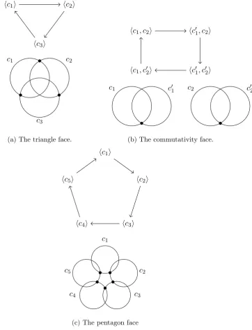
Definition 3.1. Acut systemhα₁, . . . , αgion a closed genusgsurfaceSis an unordered

collection ofgdisjoint smoothly embedded circles such that their complement is a sphere with 2gpunctures. A cut system is defined up to isotopy of the surface.

Definition 3.2. Thecut system complex is constructed as follows. Its vertices are the cut systems of S. Let hα1, . . . , αgi be a cut system. Suppose that α01 is a circle that

intersectsα1 once and is disjoint from the rest of the circles, such thathα01, α2, . . . , αgi

is a cut system. Then there is an edge from hα₁, α2, . . . , αgi to hα01, α2, . . . , αgi. The

2-cells are the triangle, commutativity and pentagon relations shown in Figure 3.1.

(30)

3.1. THE CUT SYSTEM COMPLEX

hc1i hc2i

hc3i

c1

c3

c2

(a) The triangle face.

hc1, c2i hc01, c2i

hc0₁, c0₂i hc1, c02i

c1 c0₁ c2 c0₂

(b) The commutativity face.

hc1i

hc₂i

hc3i

hc4i

hc₅i

c1

c2

c3

c4

c5

[image:30.595.125.488.172.647.2]

(c) The pentagon face

(31)

3.2. BUILDING A PRESENTATION OFH

Theorem 3.3(Theorem 1.1 [HT80]). The cut system complex is connected and simply connected.

Hatcher and Thurston show this result using Cerf theory, which we will not discuss in this thesis.

The standard cut system, C, is the cut system consisting of a meridian of each handle of the surface. LetH be the subgroup of the mapping class group that fixesC. Equivalently, this is the subgroup that fixes the corresponding vertex of the cut system complex.

We will construct a mapping class that flips an edge incident to C. Let a be the meridian of the first handle, and b be a fixed longitude of the first handle. Let C0 be the cut system consisting of a meridian of each handle except for the first handle, and a longitude of the first handle. That is,C0 =C− {a} ∪ {b}. Note that there is an edge betweenC andC0.

Definition 3.4. The mapping classσ is TaT_b−1Ta.

This is the identity outside a neighbourhood of the first handle, so fixes the merid-ians of all other handles. On the first handle, one can verify that σ takes the curve a tob and takesb toa. Thus, σ(C) =C0 and σ(C0) =C.

Given a finite presentation of H and such an element σ, which allows us to flip an edge in the complex, we can give a finite presentation of the mapping class group (Theorem 2.2, [HT80]). We will discuss this further in Section 3.3.

The authors give the construction of the full presentation quite explicitly. However, for developing the presentation of H, they give only the essential steps, and leave the construction of the presentation itself to the reader. In [Waj99], the author gives an ex-plicit presentation ofH following [HT80], but this employs only elementary techniques and does not directly use the fibrations used to construct the exact sequence in [HT80]. We will show how to apply an exact sequence to construct an explicit presentation for H genus one and two surfaces by directly following Hatcher and Thurston’s argument.

3.2 Building a presentation of

H

Using theP ushmap (Definition 2.21), we describe how to construct a presentation for H in the general case, following [HT80], and then apply this to give explicit presenta-tions for genus one and two.

3.2.1 The key steps in the H presentation

(32)

There is a fibration [HT80, Proof of Prop. 2.1]

Diff+(Srel{αi}) Diff+(S)

Diff({αi})

restriction p

which induces a long exact sequence in homotopy groups [Hat01, Theorem 4.41] ending with

π1(Diff({αi}))→π0(Diff+(Srel{αi}))→π0(Diff+(S,{αi}))→π0(Diff({αi}))→0.

(3.1) Lemma 2.4 [HT80] shows that π0(Diff+(S, α)) is isomorphic to H. Proposition 2.1

[HT80] states this exact sequence is equivalent to

Z→Zg⊕P2g−1 →H→ ±Σg →0. (3.2)

We describe how to extract a presentation from an exact sequence.

Lemma 3.5 (Lemma 28 [Waj99]). Let 0 → A → B → C → 0 be an exact sequence, with A and C finitely presented groups. Let ha₁, . . . , an|r1, . . . , rmi be a presentation

of A, andhc1, . . . , ch|s1, . . . , sgi a presentation of C. Then we get a presentation of B

as follows.

Let αi be the image of ai in B. Letγj be a fixed choice of element ofB that is sent

to cj in C. For each relation rk of A, which is a word in the ai, let tk be the word in

the αi that is the image of the word rk under the map ai7→αi. For each relations` of

C, let u` be the image of s` under the map cj 7→γj. As u` is sent to 0 in C, it is in

the image of A in B. Thus we haveu` =v` where v` is some word in the αi. For each

αi and γj, γjαiγj−1 is also sent to 0 in C, so is equal towij where wij is some word in

the αi.

Then we have a presentation of B as follows:

B =hα_i, γj|tk, u`v_`−1, γjαiγ−j1w

−1 ij i

where the variables range as follows: 1≤i≤n, 1≤j ≤m, 1≤k≤h and 1≤`≤g.

3.2.2 Genus one case

We construct a presentation of H for genus one, following [HT80]. Let S be a torus. We have a long exact sequence, from Equation 3.1, ending with

π1(Diff(α)) γ

−

→π0(Diff+(Srelα))→π0(Diff+(S, α))→π0(Diff(α))→0.

To understand these groups, first, we consider γ :π1(Diff(α))→π0(Diff+(Srelα)). In

(33)

map from the relative homotopy group of the fibration to the homotopy group of the base space,

p∗ :π1(Diff+(S, α),Diff+(Srelα),id)→π1(Diff(α),id),

which comes from the projection in the fibration, is an isomorphism [Hat01, Theorem 4.41]. Now γ is defined as the induced map in the following diagram.

π1(Diff(α),id) π0(Diff+(Srelα),id)

π1(Diff+(S, α),Diff+(Srelα),id) γ

p∗,∼= restriction

One may easily verify that π1(Diff(α),id) is isomorphic to Z, and generated by a

rotation by 2π of α∼=S1. Then p−∗1(1) is the map

(D1, S0, s0)→(Diff+(S, α),Diff+(Srelα),id)

which has a representative sending s0 to id ands1 to P ush(α) (as in Definition 2.21).

Then the restriction map sends this map to the image of s1, which isP ush(α). Thus,

γ acts by sending nto the map induced by pushing a point on α around the curve n times.

Note that in particular, this map is isotopic to the identity if we do not fixα point-wise. Thus it is in the kernel of the induced map from inclusion π0(Diff+(Srelα))→

π0(Diff+(S, α)), as we expect from the exact sequence.

By Lemma 2.4 [HT80], π0(Diff+(S, α))∼=H. The group π0(Diff(α)) is the isotopy

classes of diffeomorphisms of α ∼= S1_{. Any map} _S1 _→ _S1 _{is homotopic to the} _nth

winding map for somen, and this map is injective only forn=±1. Thusπ0(Diff(α))∼=

Z/2∼=±Σ1.

We can now write our exact sequence as

Z−→γ π0(Diff+(Srelα))→H →Z/2→0. It remains to interpret π0(Diff+(Srelα)).

Suppose we cut S alongα. The resulting surface is an annulus, which we can write as D2−D˚1 for D1 a disk in the interior of the D2. This induces a diffeomorphism

Diff+(Srelα)→Diff(D2rel{D₁, ∂D2}).Thus

(34)

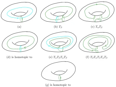
(a) (b)Tβ (c) TαTβ

(d) is homotopic to (e)TαTβTαTβ (f) TβTαTβTαTβ

[image:34.595.86.467.115.401.2]

(g) is homotopic to

Figure 3.2: Verifying thatr(α) =α−1. The green curve is the image of the given series of Dehn twists; the blue is the curve we will twist about next.

The mapping class group M od(D2 −D˚1) is isomorphic to Z and generated by a Dehn twist about the curve parallel to one of the boundary components. Thus, Diff+(Srelα) ∼=Z. When we re-glue, the generator in π0(Diff(D2rel{D1, ∂D2})) is a

Dehn twist about α.

Consider the map γ :π1(Diff(α))→ π0(Diff+(Srelα)). We have the generator of

π1(Diff(α)) going to P ush(α). But on the torus, P ush(α) is isotopic to the identity,

even if α is fixed. (We can also see this from the exact sequence, as in terms of Dehn twists about α, the generator of π1(Diff(α)) is sent to TαTα−1 which is trivial.) Thus

γ :π1(Diff(α))→π0(Diff+(Srelα)) is in fact the zero map.

Thus, we have a short exact sequence

0→_Z→H→_Z/2→0.

From this, we can build a presentation for H as described in Lemma 3.5. The generators arer, which is some element in the preimage of 1∈Z/2, andt, which is the image of 1 ∈ _Z in H. We have no relations from Z. We have r2 7→ 0 ∈ Z/2, so r2 is some word in the generators of Z. Similarly, rtr−1 7→ 0 ∈ Z/2, so rtr−1 is also some word in the generators of Z.

(35)

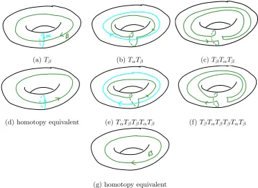
(a) Tβ (b)TαTβ (c)TβTαTβ

(d) homotopy equivalent (e) TαTβTβTαTβ (f)TβTαTβTβTαTβ

[image:35.595.131.504.116.388.2]

(g) homotopy equivalent

Figure 3.3: Verifying thatr sendsβ 7→β−1. The green curve is the image of the given series of Dehn twists; the blue is the curve we will twist about next.

α. Let r be (TαTβTα)2, for β a curve that intersects α once. By the braid relation

(Prop. 2.7), since β and α intersect once we haveTαTβTα =TβTαTβ. So

r=TαTβTαTβTαTβ =TβTαTβTαTβTα.

Since Tα(α) =α, as illustrated in Figure 3.2, we can verify this map takes α 7→ α−1.

Thus r does indeed map to 1∈_Z/2.

Since r2 fixes α, and all other curves on the torus intersect α at least once, r2 is some number of Dehn twists about α. To determine r2 in terms of Dehn twists it suffices to calculate its action on β. As illustrated in Figure 3.3, r sends β 7→ β−1. Thus r2 _{is the identity.}

Now, considerrtr−1. This fixesα so is also some word in the Dehn twists aboutα. Ast=Tα, using the braid relation we have

rtr−1 = (TαTβTα)2Tα(TαTβTα)−2

= (TαTβTαTβTαTβ)Tβ−1T

−1 α T

−1 β T

−1 α T

−1 β

=Tα

sortr−1=t, which is to say, t andr commute. Thus,

(36)

To verify this, we can describe H explicitly without using Equation 3.2, as the mapping class group of the torus is easy to describe.

It is a classical fact that M od(S)∼=SL(2,Z). Fix a meridian and longitude. Then this group is generated by the Dehn twist about the meridian, which is 1 −1

0 1

!

, and

the Dehn twist about the longitude, which is 1 0 −1 1

!

[FM12, Theorem 2.5]. The

fundamental group of the torus is generated by the meridian and longitude. If we identify them with (1,0) and (0,1) respectively, the mapping class group acts on them asSL(2,Z) acts on these vectors.

Let the fixed cut system hαi be the meridian. Note that an element a b c d

!

∈

M od(S) takes (1,0)7→ (a, c). Then the subgroup H of M od(S) that fixes (1,0) is the set that sends (1,0)7→ (±1,0) (as (−1,0) is (1,0) with the opposite orientation, and the cut system is defined up to orientation and ordering). This is the subgroup

H =

(

a b c d

!

∈M(2,Z)|ad−bc= 1, a=±1, c= 0

) = ( a b c d !

∈M(2,Z)|a=±1, d=a, c= 0

)

.

All elements of H look like

±1 b 0 ±1

!

for b ∈_Z, and we can verify that this set is closed under multiplication and inverses, since for example

1 b 0 1

!

−1 b0 0 −1

!

= −1 b 0₋_b

0 −1

!

.

Relating this back to the presentation ofH from Equation 3.2, the correspondence is

r = −1 0 0 −1

!

which reverses the orientation of both α and β, and

t= 1 −1 0 1

!

which is a Dehn twist about α.

3.2.3 Genus two case

(37)

[image:37.595.223.416.121.215.2]

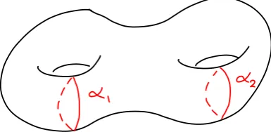
Figure 3.4: Illustrating α1 andα2 on a genus two surfaceS.

π1(Diff(α))→ π0(Diff+(Srelα)) makes the exact sequence much simpler. Genus two

is more indicative of the complexity of the general case.

LetS be the genus two surface, andα1 and α2 be the curves marked in Figure 3.4.

As with genus one, from Equation 3.1 we have a fibration inducing a long exact sequence ending with

π1(Diff({αi})) γ

−→π0(Diff+(Srel{αi})) φ

−→π0(Diff+(S,{αi})) ψ

−→π0(Diff({αi}))→0. (3.3)

Recall that by Lemma 2.4 [HT80], π0(Diff+(S,{αi}))∼=H.

Consider the map γ :π1(Diff({αi}))→ π0(Diff+(Srel{αi})) which is defined as in

the genus one case by the following diagram.

π1(Diff({αi}),id) π0(Diff+(Srel{αi}),id)

π1(Diff+(S,{αi}),Diff+(Srel{αi}),id) γ

p∗ ∼= restriction

One may easily verify thatπ1(Diff({αi}),id)∼=Z2 with generators the rotations by 2π about α1 and α2. Then p−∗1(n, m) has a representative

φn,m : (D1, S0, s0)→(Diff+(S,{αi},Diff+(Srel{αi}),id)

sending s0 to id and s1 to P ush(α1)m◦P ush(α2)n. Thus γ sends (1,0) to P ush(α1)

and (0,1) toP ush(α2). Note that these P ush maps are trivial if we fix {αi} as a set,

rather than pointwise. Thus, as we would expect, imγ is sent to 0 in H by φ. Also note that γ is injective, which allows us to rewrite Equation 3.3 as

0→π1(Diff({αi})) γ

−

→π0( Diff+(Srel{αi})) φ

(38)

Now, considerπ0(Diff+(Srel{αi})). Suppose we cutS along{αi}. We get a sphere

with four boundary components, which we can write as D2− {D˚1,D˚2,D˚3} where the

Di are disks embedded in D2. Note that any diffeomorphism of S that fixes the αi

pointwise can be interpreted as a diffeomorphism of D2− {D˚i}, so

π0(Diff+(Srel{αi}))∼=π0(Diff(D2rel{D1, D2, D3, ∂D2})).

To find π0(Diff(D2rel{D1, D2, D3, ∂D2})), note that there is a fibration

Diff(D2rel{D₁, D2, D3, ∂D2}) Diff(D2rel∂D2)

B

g

whereB is the space of orientation-preserving embeddings of three disjoint disks in ˚D2

[HT80, Proof of Lemma 2.5]. The map g : Diff(D2rel∂D2) → B is given by sending a diffeomorphism φ to the embedding sending the first disk to φ(D1), the second to

φ(D2) and the third to φ(D3). From the fibration, we get a long exact sequence in

homotopy groups:

π1(Diff(D2rel∂D2))→π1(B) ξ

−

→π0(Diff(D2rel{D1, D2, D3, ∂D2}))

→π0(Diff(D2rel∂D2)). (3.5)

We use two statements from the proof of Lemma 2.5 [HT80]. First, Diff(D2rel∂D2) is contractible. Thus the isotopy classes of diffeomorphisms and the fundamental group of this space are trivial, so, in Equation 3.5,ξ is an isomorphism. Thus

π1(B)∼=π0(Diff(D2rel{D1, D2D3, ∂D2})).

Second,B is weakly homotopy equivalent to [SL(2,R)]3×P( ˚D2; 3) by the following map. Let f ∈ B be an embedding. The weak homotopy equivalence sends f to (d1, d2, d3,{c1, c2, ci}), defined as follows. A pointci is the image of the centre of the

ith disk under f. A matrix di is the gradient of f at the centre of the ith disk.

From these statements, we have

π0(Diff(D2rel{D1, D2, D3, ∂D2}))∼=π1(B)

∼

=π1([SL(2,R)]3×P( ˚D2; 3)) ∼

=Z3×P3.

With these results, we can rewrite Equation 3.4 as

0→_Z2 −→γ _Z3×P3 φ

(39)

Consider the image of the generators of π1(B) under ξ. The fundamental group of

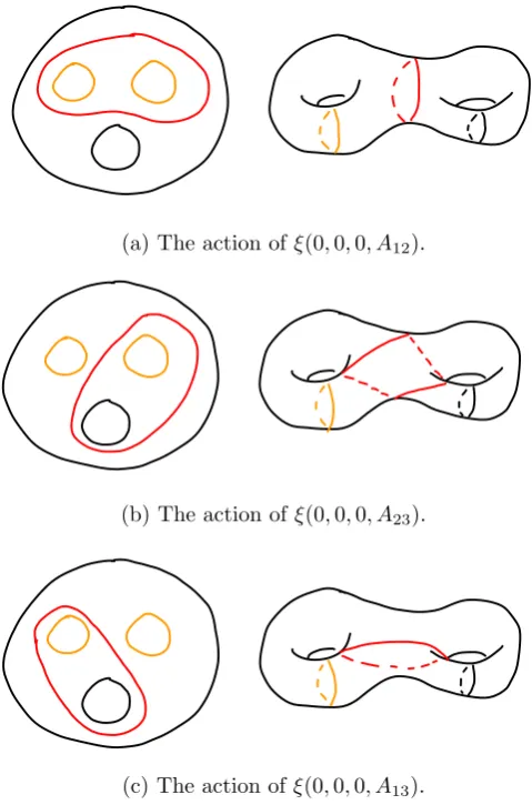
SL(2,R) is isomorphic toZ, and is generated by the loopg:S1→SL(2,R) sendingθto the matrix rotating the plane byθ. InB,ξ(1,0,0, e) then corresponds to a full rotation of the embedding of the first disk. Thusξ(1,0,0, e) is a Dehn twist about the boundary of first disk. Similarly,ξ(0,1,0, e) andξ(0,0,1, e) are Dehn twists about the boundaries of the second and third disks respectively. When we glue upD2−{D˚1,D˚2,D˚3}to make

the genus two surface, we get ξ(1,0,0, e) mapping to Tα1, ξ(0,1,0, e) mapping to T −1 α1 and ξ(0,0,1, e) mapping to Tα2. The Dehn twist about the boundary of the disk goes toT_α−₂1. See Figure 3.5 for some examples of how the disk glues up.

From the presentation of P3 in Proposition 2.18, P3 is generated by A12 = σ12,

A23=σ22, andA13=σ2σ21σ

−1

2 . The two relations are

A13A23A12=A23A12A13 and

A13A23A12=A12A13A23.

Consider the image of A12 under ξ. In configuration space, this loop is a rotation

of two points around each other. In π1(B), this is a rotation of the first and second

disks around each other, as illustrated. This is a Dehn twist about the circle separating the first and second disks from the third and the boundary. Now, ξ(0,0,0, A12) is a

Dehn twist about the loop illustrated in red on the right in Figure 3.5a. Similarly, ξ(0,0,0, A23) andξ(0,0,0, A13) are Dehn twists about the red loops in Figure 3.5b and

c.

Now, recall γ :π1(Diff({αi}))→π0(Diff+(Srel{αi})) sends (1,0) toP ush(α1) and

(0,1) to P ush(α2). Asα1 is a simple closed curve, P ush(α1) ist+t−−1, where t+ is the

Dehn twist aboutα1 pushed off to the right, and t− is the Dehn twist aboutα1 pushed

off to the left. When we cut alongα1 and α2,t+ is the Dehn twist aboutD1 and t− is

the Dehn twist about D2. Thus γ(1,0) is TD1T −1 D2 on D

2 _{with an embedding of three}

disjoint disks. Similarly, γ(0,1) is T_∂D2T_D−1

3. Thus in Z

3_×_P

3, γ(1,0) = (1,−1,0, e),

and γ(0,1) = (0,0,1, A−₂₃1A12) (sinceA−231A12 is the Dehn twist about∂D2).

We can take the quotient of the groups in Equation 3.6 by (1,0)∈π1(Diff({αi})) and

its image. This is only (1,−1,0, e)∈π0(Diff+(Srel{αi})), as by exactness (1,−1,0, e)7→

0 ∈H. ThenZ2/h(1,0)i ∼=Z and Z3×P3/h(1,−1,0, e) ∼=Z2×P3. Thus from

Equa-tion 3.6, we have the exact sequence

0→_Z−→γ _Z2×P3 φ

−→H−→ψ π0(Diff({αi}))→0 (3.7)

with the map γ :Z→Z2×P3 taking 17→(0,1, A−231A12).

As shown in Lemma 2.13, π0(Diff({αi})) ∼= ±Σ2, the group of symmetries of a

square. A presentation of this group is

(40)

(a) The action ofξ(0,0,0, A12).

(b) The action of ξ(0,0,0, A23).

[image:40.595.153.393.121.484.2]

(c) The action ofξ(0,0,0, A13).

Figure 3.5: The actions of the generators of the permutation group underξ. On the left is D2− {D₁, D2, D3}. The element ξ(0,0,0, Aij) is a Dehn twist about the red curve.

On the right, we show how this glues to make the genus two surface.

On the square, f is a flip and r a rotation by π/2. As elements of ±Sym₂, these act as f sending 1 7→ −1 and 2 7→ 2, and r sending 1 7→ 2 and 2 7→ −1. The map ψ:H →π0(Diff({αi})) is induced by restriction of S to{αi}.

From these results, we have the exact sequence

0→Z−→γ Z2×P3 φ

−→H−→ ±Symψ 2 →0 (3.8)

from Equation 3.7, as we expect from Equation 3.2.

(41)

We have generators

gTD₁, gTD₃, gA12, gA13, gA23, gf andgr

where the first five are the images of the generators of Z3×P3 under φ, and the last

two are some choice of elements ofH that get sent tof andr respectively byψ. From the relations in Z2×P3, we have relations

gA13gA23gA12g −1 A13g

−1 A12g

−1 A23 gA13gA23gA12g

−1 A23g

−1 A13g

−1 A12 [gTD₁, gA12] [gTD₁, gA23] [gTD1, gA13] [gTD3, gA12] [gTD₃, gA23] [gTD₃, gA13] [gTD₁, gTD₃].

We know the map γ :Z → Z2×P3 takes 1 7→ (0,1, A−231A12). Thus the image of

this map is generated by (0,1, A−₂₃1A12), so by exactness this gives us the relation

g−_T1 D₃g

−1

A23gA12 = id inH, that is, gTD₃ =g

−1

A23gA12. Thus we can discard gTD₃ as a generator. We are then reduced to the relations

−1 A12g

−1

A23 (3.9)

−1 A13g

−1 A12 [gTD1, gA12] [gTD1, gA23] [gTD₁, gA13] [g_A−1

12gA23, gA12] [g_A−₁₂1gA23, gA23] [g−_A1

12gA23, gA13].

Let the curves a,b, c and dbe as in Figure 3.6. Note that gTD1 isTa, and gTD3 is Tb. We choose gf and gr to be

gr=TdTb−1TaTd

(42)

Figure 3.6: The curves a (blue), b (green), c (pink) and d (green) on the genus two surface.

One can check that these act on α1 and α2 as we expect, withgr sendingα1 toα2 and

α2 toα−11, and gf reversing the orientation ofα1 and fixing α2.

From Lemma 3.5, each of

g_f2, gfgrgfgr, gfgTD₁g −1

f , gfgA12g −1

f , gfgA13g −1

f , gfgA23g −1 f ,

grgTD₁g −1

r , grgA12g −1

r , grgA13g −1

r andgrgA23g −1

r (3.10)

is equal to some words in the generators corresponding to generators ofZ2×P3, giving

us another ten relations. We will not compute these relations, as it is a tedious and uninsightful computation.

Wajnryb’s calculation [Waj99, Prop. 27] also gives an explicit set of relations for H, though with a slightly different set of generators. To give a sense of what our final ten relations would be, we express those of his relations that correspond to these ten words in our generators. They are the following:

g2_r =gA13gA23gA12(g −1 A12gA23)

−2_g−2 TD₁

g_f2 =gA23g −4 TD₁

gfgrgfgr =gA223g −4 TD1(g

−1 A12gA23)

4_(g

A13gA23gA12) −2

gfgTD₁g −1

f =gTD₁ gfgA12g

−1

f =gA13 gfgA13g

−1 f =g

2

A23gA12g −2 A23

gfgA23g −1

f =gA23g −3 TD1

grgTD₁g −1

r =gA−121 gA23 grgA12g

−1

r =gA12 grgA13g

−1

r =gA−121 g −1 A23g

−1 A13g

−1

A12gA13gA23gA12gA13 grgA23g

−1

r =grg−_A₁₂1 g_A−₁₃1g_A−₂₃1g−r1gA23gr(grg −1 A12g

−1 A13g

−1 A23)

(43)

3.3. CONSTRUCTING A PRESENTATION OF THE MAPPING CLASS GROUP

In summary, we have the mapping class group of the genus two surface generated by

gTD₁, gA12, gA13, gA23, gf and gr

with relations those listed in Equation 3.9 and the ten relations coming from Equa-tion 3.10.

3.3 Constructing a presentation of the mapping class group

We now discuss how to use these presentations of a designated subgroup of the mapping class group to construct a presentation for the whole group. Letσbe the mapping class that takesC toC0 from Definition 3.4.

Theorem 3.6(Theorem 2.2 [HT80]). Letφbe a mapping class. Thenφcan be written as a word in elements pi of H and σ, of the form φ=p1σ· · ·σpkσpk+1.

To prove this, we first show the mapping class group acts transitively on the com-plex.

Lemma 3.7. The mapping class group acts transitively on the vertices of the cut sys-tem, and H acts transitively on the edges incident to C.

Proof. The mapping class group acts transitively on the vertices of the cut systems. We can see this as follows. Cutting along the cut system gives a sphere with 2g holes. This is homeomorphic to any other such sphere, and we can pick how this homeomorphism acts on the boundary components.

Also,H is transitive on the edges incident to the vertexCin the complex. Letwbe a vertex at the end of an edge incident to C. So wis a cut system with all the curves in the cut system the same as those in C, except for one, β, which intersects αi ∈ C

once. Letz be another such vertex, which has a curveγ that intersectsαj ∈C once.

Cut the surfaceS open alongC∪ {β}. We get a sphere with 2g−1 holes. Eachαk

becomes the boundary of two holes, except for αi, where we get a hole with boundary

αiβα−i 1β−1. We get an analogous picture if we cut along C∪ {γ}. Then there is a

homeomorphism between the two spheres with boundary that takes the two boundary components corresponding toαk to each other, for allk6=i, j, and takes the boundary

αiβα−i 1β−1 toαjγα−j1γ−1. The remaining boundary components are those

correspond-ing to αj after we cut C∪ {β}, and those corresponding to αi after we cut C∪ {γ}.

Map these to each other.

This homeomorphism fixesC as a set, though it exchangesαi andαj. Thus it is in

(44)

Proof of theorem. We have fixed our standard cut system C. Recall thatσ(C) =C0. As the cut system complex is connected, there is an edge path (C=v0, v1, . . . , vn=

φ(C)) where the vi are pairwise-adjacent vertices. We build the word forφin elements

of H and σ as follows. First, as H is transitive on the edges incident to C, there is somep1∈H takingC0 tov1 and fixing C. Then p1σ takes C tov1 and C0 toC.

We have (p1σ)−1takingv2to somev10, which is connected by an edge to (p1σ)−1(v1) =

C. Then pick some p2 ∈ H taking C0 tov10, so p1σp2σ takes C to v2. We can repeat

this process to get some word p1σ· · ·pkσpk+1 such that p1σ· · ·pjσ takes C tovj.

Note that H(p1σ· · ·pkσpk+1)−1 fixes C, so is some element f of H. Thus H =

f p1σ· · ·pkσp−_k+11 with f p1∈H.

Thus, the mapping class group is finitely generated by the generators ofH andσ. It remains to find the relations betweenσ and the generators ofH. Hatcher and Thurston give explicit classes of relations between σ and the generators of H by analysing the five types of ways in which two of these words in H and σ may represent the same mapping class. These are as follows, where the square, triangle, and pentagon relations are as in Figure 3.1:

1. The two words are different words corresponding to the same path.

2. The two words correspond to paths that differ by an involution. For example, if one path of edges ise1e2e3, the other might bee1e2e4e−41e3.

3. The two words differ by a triangle relation.

4. The two words differ by a square relation.

5. The two words differ by a pentagon relation.

The corresponding five classes of relations are as follows.

Theorem 3.8(Theorem 2.2 [HT80]). All relations between words of the formp1σ· · ·pkσpk+1

as mapping classes follow from the following five classes of relations. These relations correspond to the five ways in which two of these words may represent the same mapping class.

1. The letter σ commutes with the subgroup of M od(S) that fix both C and C0 = σ(C), which one can show is finitely generated.

2. The elementσ2 is in H.

3. For a finite set of pγ in H, (pγσ)3∈H.

(45)

5. For a finite number of choices of p0, p1, . . . , p4, σp4σp3· · ·σp0 is inH.

(46)

(47)

Chapter 4

Marked Bordered Fatgraphs and

Their Duals

A marked bordered fatgraph (Definition 4.16) is an embedding of a certain class of graph in a surface such that its complement consists of one contractible piece for each boundary component. The dual graph to this is embedding is a quasi-triangulation. Quasi-triangulations consist of monogons (each of which contains one boundary compo-nent) and interior triangles. As in Chapter 3, we can consider the mapping class group action on a surface S decorated with one of these objects. In this case, the action is free (Proposition 4.26).

In this chapter, we will define a marked bordered fatgraph and prove some results on its dual. Principally, we will show that the mapping class group acts freely on marked bordered fatgraphs, and we will give an algorithm to associate a minimal generating set for the fundamental path groupoid to a marked bordered fatgraph. In Chapter 5, this will allow us to define a marked bordered fatgraph complex (Theorem 5.5) with a naturalM od(S)-action, giving us an infinite presentation of a mapping class groupoid in terms of moves on bordered fatgraphs.

We will use this presentation in Chapter 6 to give a finitely generated presentation of the same groupoid in terms of chord slides on chord diagrams whose chords are the minimal set of generators for the fatgraph. This will induce an infinite presentation of the mapping class group. Sections 4.1-2 follow [God07].

4.1 Defining

n

-bordered Fatgraphs

4.1.1 Fatgraphs

First, we establish a convention for formally describing graphs.

(48)

[image:48.595.206.351.124.270.2]

4.1. DEFININGN-BORDERED FATGRAPHS

Figure 4.1: An example of a fatgraph.

two maps, v : ξor(G) → V(G) and an involution i : ξor(G) → ξor(G) that fixes no

elements.

We interpret the setV(G) as the vertices of the graph, andξor(G) as the oriented

edges. Then v sends an oriented edge e to the vertex it points to, and i sends an oriented edge to the same edge pointing in the opposite direction. As shorthand, we use the notatione=i(e). To avoid ambiguity,ac, for instance, isi(a)i(c) (that is, the order does not reverse as it does with inverses).

We assume a basic knowledge of graph theory. For full definitions, see [Die00]. Our definition of a graph is equivalent to Diestel’s definition of a graph, by sending one of our edges eto the edge (v(e), v(e)). Our notation, however, allows us to easily refer to an edge with a particular orientation.

Definition 4.2. A morphism of combinatorial graphs, ψ : G → G, is a map of setse

ξor(G)∪V(G) → ξor(G)∪V(G) such that for any oriented edge e of G,e ψ−1(e) is a

single oriented edge of G, and for any vertexv of G,e ψ−1(v) is a tree.

Definition 4.3. Afatgraph Γ is a connected combinatorial graph with a permutation σ of the oriented edges ξor(Γ) that restricts to a cyclic ordering of the edges pointing

to each vertex.

Given an oriented edge e, we sayi◦σ(e) is the consecutive edge. This is the next edge in the ordering aroundv(e) but pointing away from the vertex rather than towards it.

Definition 4.4. A fatgraph morphism is a morphism of combinatorial graphs that respects the cyclic ordering on edges at a vertex.

(49)

[image:49.595.225.409.120.250.2]

Figure 4.2: A fatgraph with two boundary cycles, each coloured.

example, see Figure 4.1. When we draw fatgraphs, we will draw them such that this is their cyclic ordering.

Definition 4.5. A boundary cycle of a fatgraph Γ is a cycle of consecutive oriented edges, that is, a cycle of the permutationi◦σ.

For example, see Figure 4.2, which has boundary cycles outlined in blue and pink.

4.1.2 Bordered Fatgraphs

We wish to consider a subclass of fatgraphs that arises as the dual of quasi-triangulations.

Definition 4.6. A bordered fatgraph is a fatgraph with an ordering on the boundary cycles satisfying the following conditions.

• First, there is precisely one univalent vertex in each boundary cycle, called the tail vertex. The single edge incident to it is called the tail.

• All vertices that are not tail vertices are trivalent.

A bordered fatgraph is n-bordered if it hasn boundary cycles.

Figure 4.2 is an example of a twice-bordered fatgraph. In Theorem 5.5, we will show that it suffices to consider these n-bordered fatgraphs to get a presentation of M od(S). To prove this, we will need a generalisation of a bordered fatgraph, where some edges have been collapsed.

(50)

Definition 4.8. Let Γ be a collapsedn-bordered fatgraph. Supposeeis an (unoriented) edge of Γ. The preferred orientation ofeis the orientation in which we first traverse it in the following procedure.

Starting at the first tail vertex, follow the first boundary cycle around the graph until you return to this vertex. Then repeat this for the second throughnthtail vertices in order.

Lemma 4.9. There is at most one fatgraph isomorphism between any two collapsed bordered fatgraphs that preserves the ordering of the boundary cycles.

Proof. Note the inverse of such a fatgraph morphism also preserves the ordering of the boundary cycles.

First, we show that the only automorphism of a collapsed bordered fatgraph fixing the boundary cycle ordering is the identity. Such an automorphism must preserve the valency of the vertices (as every edge is sent to exactly one edge), so in particular sends the set of tail vertices to the set of tail vertices.

The ith boundary cycle is a cycle of i◦σ. The elements of this cycle are mapped bijectively to another cycle of i◦σ, which must be the same cycle by the preservation of the ordering on boundary cycles. Then once we find the image of one element in the cycle, we have determined the images of all the elements in the cycle (as the relationship of consecutive edges is preserved). Now, the unique tail vertex in this boundary cycle must be sent to a tail vertex, so in particular is sent to the tail vertex of this boundary cycle. Thus, the map is the identity on theithboundary cycle for alli, so is the identity on the entire fatgraph.

Now, suppose there were two isomorphisms fixing the boundary cycles,φ1 andφ2,

from Γ1 to Γ2. Then φ−1◦ψ: Γ1 →Γ1 is an automorphism that is not the identity, a

contradiction.

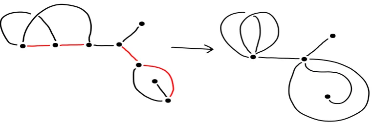
We now define a morphism of collapsed bordered fatgraphs as a forest collapse.

Definition 4.10. Let Γ be an n-bordered fatgraph. Let F ⊂ Γ be the union of a pairwise disjoint set of trees of the graph (a forest), such that F does not contain any of the tails. The forest collapse of F acts by collapsing each connected component of F to a vertex.

An example of a forest collapse is shown in Figure 4.3.

Definition 4.11. A morphism of collapsed bordered fatgraphs ψ : Γ1 → Γ2 is a

com-position of forest collapses and boundary cycle-preserving isomorphisms.

(51)

[image:51.595.121.502.117.243.2]

Figure 4.3: A morphism of collapsed twice-bordered fatgraphs, collapsing the forest in red.

Definition 4.12. We say ψ1 : Γ1 → Γe₁ is equivalent to ψ₂ : Γ₂ → Γe₂ if there exist

isomorphismsθ: Γ1 →Γ2 and θe:eΓ₁ →Γe₂ such that the following diagram commutes.

Γ1 Γe₁

Γ2 Γe₂

ψ1

ψ2

θ eθ

From here, all isomorphisms between collapsed bordered fatgraphs will be boundary cycle order-preserving isomorphisms. We will say a collapsed bordered fatgraph to mean an equivalence class of collapsed bordered fatgraphs, up to one of these isomorphisms.

Remark 4.13. We can more generally define a collapsed bordered fatgraph morphism as a fatgraph morphism preserving the boundary cycle ordering. On equivalence classes of these fatgraphs, this is equivalent to our definition of these fatgraph morphisms being forest collapses [God07, Lemma 3].

In the following lemma, we show we can compose (equivalence classes of) morphisms of collapsed bordered fatgraphs in a well-defined manner.

Let ψ : Γ1 → Γ2 and φ : Γ3 → Γ4 be collapsed bordered fatgraph morphisms,

with Γ2 and Γ3 in the same equivalence class. Then there is a (unique) isomorphism

θ between Γ2 and Γ3. We define the composition of the equivalence classes of these

morphisms, [φ]◦[ψ], to be the equivalence class of the composition

Γ1 ψ

−−−−→Γ2 θ

−−−−→Γ3 φ

−−−−→Γ4.

Lemma 4.14. This composition is well-defined.

Proof. We give the case of two equivalent morphisms Γ1→Γ2, as the case for Γ3→Γ4

is very similar. Let ψ : Γ1 → Γ2 and ψe : Γe₁ → Γe₂ be equivalent morphisms, with

(52)

4.2. MARKED BORDERED FATGRAPHS

Supposeψ: Γ3→Γ4 with Γ3 and Γ2 isomorphic so composition is well-defined. As

Γ2∼=Γe₂, there is a (unique) isomorphismθe:Γe₂ →Γ₃. Then we wish to show that the

following diagram commutes.

Γ1 Γ2 Γ3 Γ4

e

Γ1 eΓ₂ Γ3 Γ4

ψ _θ

∼

=

φ

e

ψ _θ_e

∼

=

φ

θ1 ∼= θ2 ∼= id id

The rightmost square commutes trivially, and the leftmost commutes as ψ and ψeare

equivalent morphisms. Then as θeis the unique isomorphism Γe₂ → Γ₃, we have θe=

θ◦θ−₂1 since this is also an isomorphism between these fatgraphs. Thus, the middle square commutes, soφ◦θ◦ψ and φ◦θe◦ψeare equivalent morphisms.

4.2 Marked bordered fatgraphs

Let Σg,n be the genus g orientable surface withn boundary components, with a fixed

ordering on the boundary components and a marked point on each boundary compo-nent. We will now view n-bordered fatgraphs as embedded in Σg,n for some g, and

use this to construct a category of these embedded fatgraphs, EF atg,n, with a natural

action of M od(Σg,n).

Suppose we embed ann-bordered fatgraph as a spine in a surface withnboundary components, which we will formally define in Definition 4.16. Let the number of vertices of Γ be V, and the number of edges be E. We can view the surface as a thickened version of the fatgraph, motivating a definition of the genus of the fatgraph. We can construct the surface as a neighbourhood of the fatgraph as follows. We thicken each edge of the fatgraph to a rectangle with four edges, two of which are on the boundary, and each vertex to a triangle with three edges and three vertices. We can then calculate

2−2g−n=χ(ΣΓ) = 3V −(3V + 2E) + (V +E) =V −E =χ(Γ).

This motivates the following definition.

Definition 4.15. The genus of an n-bordered fatgraph Γ is the numberg such that χ(Γ) = 2−2g−n.

We will restrict our attention to the set of (isomorphism classes of) collapsed n-bordered fatgraphs of genusg,F atg,n. Then these are precisely the collapsed bordered

fatgraphs that embed into Σg,n as a spine, that is so that the complement of the