Simulation and analysis of a digital scanning system

Rochester Institute of Technology

RIT Scholar Works

Theses

Thesis/Dissertation Collections

1990

Simulation and analysis of a digital scanning system

Eugene A. Rogalski

Follow this and additional works at:

http://scholarworks.rit.edu/theses

This Thesis is brought to you for free and open access by the Thesis/Dissertation Collections at RIT Scholar Works. It has been accepted for inclusion

Recommended Citation

Simulation and Analysis of a Digital Scanning System

by

Eugene A. Rogalski, Jr.

A Thesis Submitted

in Partial Fulfillment

of the

Requirements for the Degree of

MASTER OF SCIENCE

in Mechanical Engineering

Approved by:

Prof.

Joseph S. Torok

(Thesis advisor)

Prof.

Prof.

P Venkatar

Prof.

Wayne W. Walter

Mr.

Thaddeus Kciuk

Prof.

B.

Karlekar

(Department Head)

Department of Mechanical Engineering

College of Engineering

Rochester Institute of Technology

Rochester, New York

Simulation

and

Analysis

of

a

Digital

Scanning

System

I,

Eugene

A.

Rogalski,

Jr.

hereby

grantpermission

to the

Wallace

Memorial

Library,

of

the

Rochester Institute

of

Technology

to

reproduce

my

thesis

in

wholeorpart.

Any

reproduction willnot

be for

commercial use or profit.

Acknowledgment

This

work could not

have

been

possible without

the

supportandguidance of

several

individuals.

Its

success

is due

largely

to their

encouragementand

suggestions

and

I

extend

my

deepest

appreciation:

To Xerox

Corporation

for

the

useof

computing

facilities.

To

Dr. Wayne

Walter,

Dr.

P.

Venkataraman,

and

Dr.

Hany

Ghoneim for

taking

time

outof

their

busy

schedules

to

read and critique

my

work.

To Michael Boyack

who

designed

the

control system which was used

in

this

analysis

and who provided

the

controls

hardware

and software.

His

enthusiasm

for

the

design

and analysisof controlsystems wasan

inspiration.

To

Thaddeus

Kciuk

who providednumerous suggestions and guidance.

To Dr. Joseph

Torok,

Rochester

Institute

of

Technology,

Department

of

Mechanical

Engineering

for

his

very

functional

guidance andencouragement.

And

lastly,

though

notatall

last,

to

my

wife

Marlene

whosupplied

Abstract

The

analysis

and simulation of

the

motion of a

digitally-controlled digital

imaging

system

is

presented.

The

dynamic

system consists ofa

scanning

carriage,

power

transmission

elements,

a prime

mover,

andacontrol

subsystem.

The

prime mover

is

apermanent magnet

DC

motor

that

is

positioned

by

a

direct

digital

control system.

The

scan carriage motion

is

mathematically

modeledand simulated

using ACSL

and

DADS

simulation

software.

T

he

simulationresultsare compared

to

empirical

data.

It is

shown

that

the

dynamic

response of

the

actualscan system can

be

predicted quite

well

using

suchsimulations.

Furthermore,

these

simulations can aid

in

the

Table

of

Contents

Page

List

of

Tables

vi

List

of

Figures

vii

List

of

Symbols

ix

I

Introduction

1

II

Control System

Preliminaries

11

III

Description

of

the

Physical

System

24

IV

Mathematical

Modeling

28

V

Simulations

42

VI

Results

44

VII

Conclusions

55

VIII

References

58

List

of

Tables

Page

1.

Full Model

Step

Response

Comparison

47

2.

Physical Constants

69-70

List

of

Figures

Page

1.

Building

Blocksof

a

Digital

Scanning

Device

2

2.

Imaging

Definitions

3

3.

Contrast

Sensitivity

of

the

Human Eye

to

Square Wave Gratings

5

4.

Perceptibility

Threshold

of

Edge

Raggedness

6

5.

Motion Error

Detectability

-Threshold

Design Goal

8

6.

Velocity

Error Design Goal

9

7

Basic Components

of a

Closed

Loop

Control System

11

8.

Nonlinear

Element

12

9.

Linearity

Improvement

13

10.

Block Diagram

Transfer Function

15

11.

Block Diagram

Reduction

17

12.

Digital

Control

System

19

13.

Uniform

Sampler

19

14.

Sampler

with

Zero Order Hold

20

15.

Physical

System

24

16.

Control

System

/Mechanical

Block

Diagram

25

List

of

Figures

(continued)

Page

18.

Controls

Block Diagram

29

19.

Motor

Circuit

31

20.

Simple Mechanical

Model

Block Diagram

35

21.

Lumped Parameter

Mathematical Model (Translational

DOF)

38

22.

Linearized Lumped

Parameter Model

(all

DOF)

39

23.

Eigenvalues,

Eigenvectors

and

Mode

shapes

for

3 DOF

model

41

24.

Simple

Model Motor

Step

Response

ACSL Simulation

45

25.

Simple

Model Motor

Step

Response

DADS Simulation

45

26.

Full Model Motor

Step

Response

ACSL Simulation

46

27.

Motor

Step

Response

Experimental Result

46

28.

Motor/ Carriage

Ramp

Response

-ACSL

Simulation

48-49

29.

Motor/ Carriage

Ramp

Response

Experimental Result

50

30.

Motor

Ramp

Response Increased

Sampling

Period

52

-ACSL

Simulation

31.

Motor

Ramp

Response Increased

Sampling

Period

52

-

Experimental

Result

32.

Mechanical

Frequency

Response

53

List

of

Symbols

a;

Linear

acceleration, ith

element

B

Viscous

damping

coefficient

c

Command

position

Cj

Viscous

damping

coefficient

ek

discrete

error

kth

sample

f

Position

feedback

Ffj

Linear

friction

G

Plant Transfer Function

H

Feedback Transfer Function

ia

Armature

current

li

Inertia

lm

System

inertia

Kd

Derivative

gain constant

Ke

Generated

back

EMF

constant

K,

Spring

constant,

ith

element

Kp

Proportional

gain constant

Kj

Motor

torque

constant

La

Motor

armature

inductance

Mj

Mass,

ith

element

Nenc

Encoder

line

density

R

Result-Ouput

Ri

Radius

of

the

ith

element

Rc

Capstan

radius

Rm

Motor

armature resistance

s

Laplace Variable

Tfj

Torsional

friction

TmotorTorque

produced

by

motor

Tres

Resultant

Torque

Ts

Sampling

time

List

of

Symbols

(continued)

Va

Applied

motor voltage

vi

Linear velocity

Vb

Generated

back

EMF

voltage

Vm

Motor

armature

voltage

xj

Linear

position

z

Z Transform Variable

9i

Angular

position

ai

Angular

acceleration

8(t)

Unit Impulse Function

Qi

Angular

velocity

$

Magnetic

field

flux

I

INTRODUCTION

Digital

scanners

are

taking

on an ever

-increasing

role as

input

devices

to

computer-based

systems.

As

typical

optical

disk

storage

capacities

exceed

1

Gigabyte

and

desktop

publishing

equipment

rivals print

shop quality,

digital

scanners are

becoming

a popular

computing accessory for

data

storage,

and

image

manipulation

purposes.

Acting

as

a

link between

the

paper and

electronic

worlds, the

input

scanner

creates

an electronic

image

of

the

paper

original which

is

then

processed

according

to

the

user's requirements.

Downstream

processing

may include intelligent

character recognition

for

text

input

and subsequent

word

processing

applications,

enhancement

for image

input,

or

file

compression

for

archival storage purposes.

The

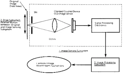
operation of

any digital scanning

device

requires

three

basic

building

blocks

as

shown

in

Figure

1

.

The

first

and

most

important block

contains

the

image

sensor and optical system.

Together

these

elements convert

the

light

and

dark

portionsof

the

original

image into

individual picture elementsor pixels.

Charged

coupled semiconductor

devices

(CCD's)

are

typically

used

as

image

sensors

in

many

scanners on

the

market

today.

The

second

building

block

assures

that

the image

sensor

physically

scans

the

input

to

create a

two

dimensional

map

of

the

original.

This

motion can

be

achieved

by

moving

the

image

sensoror

the

input document

relative

to the

other

using

a

variety

of

drive

transmission

schemes.

The

last step is

then to

process

the

two

dimensional

pixel

bitmap

into

useful

data.

Depending

upon

the

downstream

Original Image

(Side

View)"

2 Drive Subsystem Relative Motion between Original

andImage

Sensing

Subsystem

ChargedCoupled Device CCDimage sensor

Signal

Processing

Electronics

Optics

1 Image

Sensing

Subsystem

3 Image

Processing

[image:13.523.53.477.116.374.2]

Subsystem

FIGURE 1

:

Building

Blocks

of

a

Digital

Scanning

Device

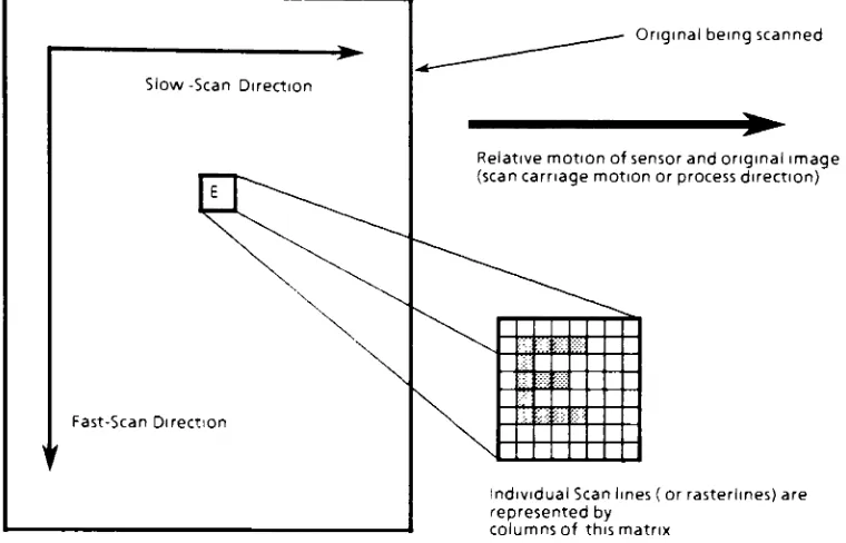
The

two

dimensional

map

of

pixels

formed

by

scanning

the

image

may

be

conveniently

thought

of

as

a

group

ofparallel

but

separate

scan

lines

each

containing

a

line

of pixels

imaged

at an

instant

in

time.

The

lines

oriented

parallel

to

a scan

line

are

said

to

lie

in

the

fast-scan

direction,

because

in this

direction

the

pixels

are

imaged

more

rapidly.

This is

the

direction

perpendicular

to

the

motion of

the

imaging

carriage

or paper process

direction.

The

slow-scan

direction is

defined

as

that

which

is

perpendicular

to

the

fast-scan direction

and

is

in the

direction

of motion of

the

carriage.

In

the

scanning

lines

of

a cathode

ray

tube.

The

above

definitions

are

illustrated

in

Figure

2

and are

further described

in

HI.

>?

Slow-Scan Direction

Fast-Scan Direction

Original

being

scanned

Relativemotion of sensor and original image scan carriage motion or process

direction)

!*"rrr. m

^

individualScan lines

(

orrasterlines)are represented

by

columnsof thismatrix

FIGURE

2:

Imaging

Definitions

Image distortion

can occurwhen either

the

fast

or slow-scan rates

are

not constant.

Perturbations

ofscan

rates

in

either

direction

cause pixels

to

be

imaged

incorrectly

and

as a result create

local

variations

in

the

reflectance

of

the image.

Random

fluctuations

in

one

direction

cause

one

dimensional

disturbances in

the

recorded

image. This

phenomenon

is

termed

"banding"

and

typically

refers

to

image

distortion

caused

by

disturbances

which occur

in

the

process

direction.

Banding

in

scanned

images

refers

to

the

fluctuations

[image:14.523.72.452.144.388.2]

output

image.

Thus,

to

faithfully

reproduce

an

input

and

keep

customer

perceptions

of

scanning devices

favorable,

vibrations

in

the

slow-scan

direction

must

be kept below

perceptible

limits

[2-3]

.

To

avoid such errors

in the

image,

the

main objective of scan mechanism

design

must

be

to

provide a

smooth, i.e.

constant,

slow-scan velocity.

However,

friction,

system

dynamics

and

other

disturbances

cause

velocity

fluctuations

and

vibrationswhich

must

be

attenuated

if

image distortions

are

to

be

minimized.

The

useof

feedback

to

control slow-scan motion

is

usually

a

necessity,

but

evenwith

the

added

robustnessofa control

system,

vibration

and

image

motion problems can still

be

present.

Additionally,

downstream

processing

and

image

output

devices

can either

magnify

or attenuate

these

errors and

like

consideration must

be

given

to these

additional

devices.

Thus

some

questions

remain, namely,

how

to

determine

the

perceptible

level

of

slow-scan motion error

and

what

is

an acceptable

level

of vibration?

Much

of

the

published work

relating to perceptibility

and motion

requirements

is

concerned with

printing

oroutput

devices,

specifically

xerographic

laser

printers

Ml.

However,

the

psycophysical experiments used

to

determine

human

vision

sensitivity to image

defects

are

still applicable

to

input

scanning devices.

Visual

perceptual phenomena

are

highly

dependent

upon a

variety

of

factors.

Variations

in

exposure

duration,

illumination,

viewing

distance,

image

significantly

shift

perceptibility

thresholds.

A

full

discussion

of

these

parameters,

the

eye's

structure,

and

the

psychology

of perception

is beyond

the

scope

of

this

work.

The

reader

is

directed

to the

appropriate references

[4-71

for

more

detailed information

on

these

subjects.

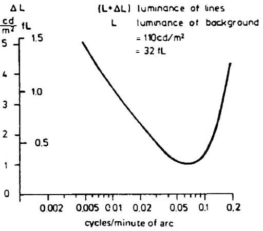
When

imaging

a

specific

pattern, if

groups

of

scanlines are

imaged

more

closely

together

or

farther

apart, the

average

reflectance of

that

region

increases

or

decreases,

respectively.

As

demonstrated

by

Hilzfs],

the

resulting

AL

cd

5

4

IL

r

1.5

(.

--

1.0

3

-2

-(L*ALl

luminance

of lines

L

luminance

of

background

- HOcd/m*

-

32

tL

0.5

I 1

|

'

'"I

_I r"

'

I ""I

1

0002

0.005 0 01

0.02

0.05

0.1

0.2

cycles/minuteofarc

FIGURE

3: Contrast

Sensitivity

of

the Human

Eye

to

Square Wave Gratings

8

periodicone-dimensional

brightness

fluctuations

and contrast

sensitivity

of

the

human

vision system related

to

local

frequency

is

depicted

in Figure

3.

Hilz's

work presents

the

eye as most sensitive

(with

respect

to

background

[image:16.523.130.386.276.501.2]

1

.2

cyc/mm

(assuming

a

300mm viewing

distance).

Bestenreiner

et

al

IU

reinforce

the

supposition

that the

detectability

of

line

lattice

interference

structures

in

recorded

images

relies

upon

the

contrast

of

the

lattice,

the

luminosity

of

the

background

and

the

spatial

frequency

of

the

lattice.

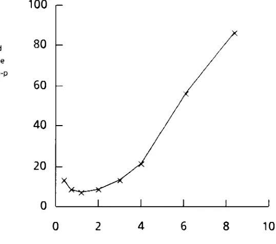
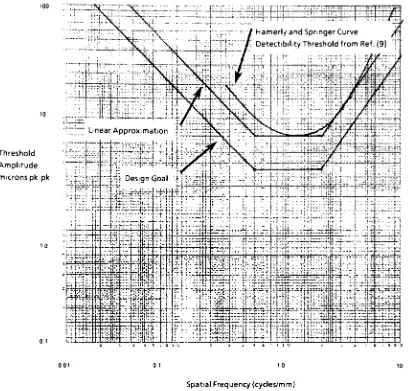
The

work of

Hamerly

and

SpringerOl

(see

Figure

4),

in

regards

to

edge

100

r-Threshold

Amplitude

microns_p-p

80

-60

-40

20

-0

8

10

Spatial

Freguency

(cycles/mm)

FIGURE

4:

Perceptibility

Threshold

of

Edge Raggedness

8

detection

and

degree

of

raggedness,

also

supports

the

presence

of

frequency

select channels

in

the

eye

which might

be

appropriate

for

describing

the

detectability

and

thresholds

of

edge

raggedness.

Figure

4

depicts

the

[image:17.523.120.389.215.453.2]

frequency

based

upon a

viewing distance

of

400mm. This

result

reinforces

Hilz'

findings

and

describes

the

eye as most sensitive

to

errors

ofspatial

frequencies

in

the

0.5

-

1

.2

cyc/mm

range.

The

previous

findingsM-9]

and

Figures

3

and

4

reinforce

the

inclination

to

develop

a

steady-state

motion specification

for input scanning

devices

with

the

spatial

or

temporal

frequency

of

the

motion

as

the

independent

variable

and

the threshold

amplitude

in

units of

displacement

as

the

dependent

variable.

Replotting

Figure

4

on a

log-log

scale

(see

Figure

5),

several

regions can

be

identified

and a

linear

approximation can

be

used

to

delineate

the

threshold

values of

perceptible

error.

Furthermore,

since

the

curve

indicates

threshold

values

(i.e.

errorswith

amplitudes above

the

curve

are

noticible

to

an

observer)

,

dividing

the threshold

by

a

safety factor

of

2

yieldsa

specification which

may

be

an

appropriate

design

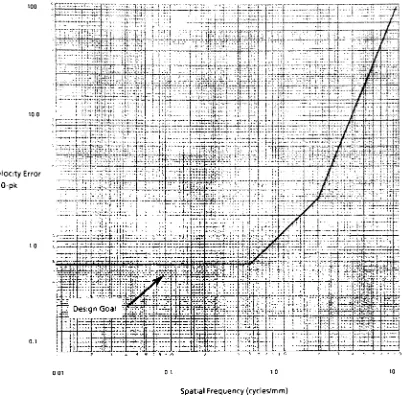
goal.

Realizing

that the

measurement

of motion

is

an

inevitable

task,

it

is

appropriate

to

express

the

perceptibility

threshold

in terms

of

velocity

error

(as

shown

in Figure

6)

to

account

for

different

sensor

types.

Refer

to

Appendix

A

for

the

conversion

from

a

displacement-based perceptibility

threshold

to

a velocity-based

perceptibility

threshold.

The

motion requirementsand

thresholds

for

many

commercial

scanning

devices

reflect

the

scanning

resolution

and

often

take

into

consideration

the

anticipated outputor

hardcopy

devices.

For example,

a

xerographic

laser

Threshold Amplitude microns pk-pk

^ 3 1

001 0.1

Spatial

Frequency

(cycles/mm)

FIGURE

5: Motion Error

Detectability

-Threshold

Design Goal

requirements

are

typically

very

stringent

to

allow

for

this

uncertainty.

It

should

be

noted

here

that

the

derivation

of

the

specification curves

is

[image:19.523.63.474.75.466.2]

100

Velocity

Error

%0-pk

y||I

Sfe

^^^^fM^^fg^

Jig

g|Mfi

,4lferfft|Ft

rHt:-'-nT3:-n^l1i:>r

;

r

Mist

*A~h:l\i\:

>!:

;. ;

Design Goal '-.!2^Ip.

-t

4t-&j*

w-i'it 2D" TTTT XXt

#tSE!;CI

13x1

CAiErfejtSitip

lit * Jtjt."

fci~ f'

;

"

-ty---rt.{.-jrtiS;'*.f;''* r.

Silt rH'~T

-i-r-n--'-tl-'"- t^^ffi^-rr-?

7* _::':^:::i ;:4...:_.:-..ai-;i4-;-. . --pif-p Si}:!a::::r r+f7'Trj '

0.1 10

Spatial

Frequency

(cycles/mm)

FIGURE

6:

Velocity

Error Design Goal

In

light

of

the

above

discussion,

the

characterization of

the

scanning

system

and measurementof motion

are

the

main

goals

in

an

analysis and

design

of

a

scanning

system.

The

motion goals

defined

in

Figures 5

and

6

are

the

specifications.

Mathematical

modeling

and simulation

tools

can

be

used

to

predict

the behavoirof

a

system

before

any

hardware

is

constructed.

These

[image:20.523.67.469.64.459.2]

analysis.

Experimental

verification

of

any

simulation

is

prudent

and

often

a

necessity.

The

goal of

this

work

then

is

to

discuss

the

basic

operation ofa

particular

scanning

system,

_perform

the

analysis and

simulations

to

predict

the

characteristics

of

that

system

and

finally,

to verify

these

predictions with

II

CONTROL

SYSTEM

PRELIMINARIES

It is

appropriate

to

engage

in

a general

discussion

of

the

mathematics

and

basic

principles

of

control systems

that

_will

be

_required

in the

_simulation

process.

Control

systems are

used

in

a wide

variety

of

applications

to

enable

a

desired

performance

of a

dynamic

system under

changing

conditions

and are

generally lumped

into

two

categories

-open and closed

loop

systems.

Open

loop

(nonfeedback)

systems are

less

robustand are

easily

affected

by

external

disturbances.

A

closed

loop

system,

on

the

other

hand,

uses

feedback

to

monitor

the

output and

is

able

to

compensate

for

external

disturbances.

Feedback

can also

be

used

to

improve

the

linearity

ofasystem and enables

it

to

be

more

robust

in

rejecting

external

disturbances.

Figure

7

shows

the

basic

componentsofa closed

loop

control system.

The

CONTnni sic;mai <;

PLANT

ACTUAL OUTPUT

COMPENSATION

UNIT

REQUIRED

'

'

OUTPUT

FEEDBACK

SENS ORS

Figure 7:Basic Components

of a

Closed

Loop

Control System

plant

defines

the

processor system which

is

to

be

controlled

and

may

contain

any

number ofcontrollable variables.

To

obtain optimal

performance

from

adjusted accordingly.

Feedback

is

provided

by

sensors

which monitor

the

variables

that

affect

the

performance

of

the

plant.

The

compensation unit

makes

a

comparison

between

the

required output and

feedback from

the

plant,

determines

if

the

error

between

them

is

within

acceptable

limits

and

then

adjusts

the

control signals

to

the

plant

to

achieve

the

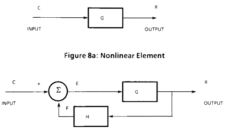
actual output.

To

examine

how

closed

loop

control

systems

can

improve

the

linearity

of a

systemtiO],

consider

the

configurations

shown in

Figure 8.

The input-output

c

G

R

NPUT OUTP

Figure

8a: Nonlinear Element

INPUT i

o

fc

G

J

' f

H

OUTPUT

Figure 8b: Nonlinear Element

with

Feedback

relationship

for

nonlinear element

G

in

Figure 8a

is

R

= C2

Figure

8b

shows

the

same nonlinear element with a

unity

gain

feedback

loop

element

H

(H

=

1).

The

equation

for

the

output

R,

in

terms

of

the

input

C

for

the

closed

loop

system of

Figure

8b

can

be developed

by

expressing

E

and

F

in

terms

of

C

[image:23.523.67.431.262.488.2]

E

=

C-F

E

=

R/G

F

=

HR

(2.1)

(2.2)

(2.3)

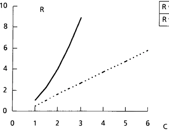
Substituting

2.2

and

2.3

for

E

and

F

in

equation

2.1

and

rearranging

yields:

R

=

CG

(2.4)

(1

+

GH)

Figure

9

plots

both

the

open

loop

and closed

loop

outputs verses

the

input

C.

The

output

R

of

the

closed

loop

case

is

more

linear

and

follows

the

input

C

more

closely

due

to

the

feedback

loop.

10

6

4

2

0

R

w/o

feedback

R

w/

feedback

Figure

9:Linearity

Improvement

Another

feature

of

using

closed

loop

control

is

that

if

designed

properly, the

system

may be

less

sensitive

to

plant variations.

If the term GH

in

the

denominator

of equation

2.4

is

made

to

be

such

that GH>

>1,

then the

[image:24.523.66.335.286.495.2]

R~

CG_

(2.5)

GH

and

further:

R

~

C_

(2.6)

H

If

GH>>1,then

variations

in

G

will

have

little

or no affect on

the

ability

of

the

control system

to

effectively

control

the

process

G

as shown

by

2.6.

The

Laplace

Transform

and

Transfer

Functions

Another

tool

that

is

used when

analyzing

and

modeling linear

control systems

is

the

Laplace

transform.

This

is the

main mathematical

tool

of

the

control

system

designer

because

it

simplifies

the

manipulation of

transfer

functions.

The Laplace

transform

relates a

function

of

time

f(t)

to

a

function

F(s)

where

the

variable,

s,

is

in

general a complex quantity.

The

transform

is

defined

by

the

definite

integral

F(s)

=

/.

{

f

(t)

>

= 0/-f(t)e-stdt

(2.7)

The

main

advantage

of

the

transform

is that

differentiation

and

integration

operations

are

changed

into

simple

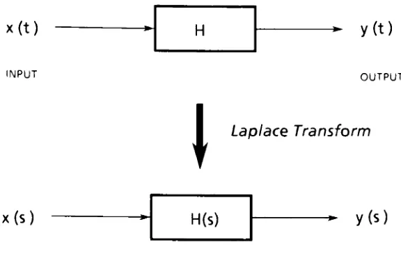
algebraic operations.

Consider

the

block

diagram

in

the

top

portion of

Figure

10.

The

generic

function

H

can represent

any

mathemathical

relationship

between

the

input

and

output.

The

function

H

could

be

a

constant value

indicating

a

linear

relationship,

a

first-order

pole or

a

complexnonlinear

function.

Applying

the Laplace

transform

to the

relations

depicted

by

this

block diagram

we

x(t)

H

y(t)

INPUT OUTPUT

\

Laplace Transform

x(s)

TRANSFORMED EXCITATION

H(s)

-

y(s)

SYSTEM TRANSFER FUNCTION rRANSFORMED RESPONSE

Figure

10: Block Diagram

-Transfer Function

y(s)

=

H(s)x(s)

(2.8)

Once

the

transfer

function

is

manipulated

to

the

proper

form

in

the

s

domain,

the

response

y(t)

of

the

system

to

an excitation

x(t)

may

be

recovered

by

the

inverse

Laplace Transformation

of

y(s)

represented

by:

y(t)

=

Z.-1

{y(s)}

=

M

{

H(s)

x(s)

}

(2.9)

Equation

2.9

can

be

used

to

derive

the

response

of

any linear

time-invariant

system subjected

to

an

arbitrary

excitation.

The Laplace

transform

of

the

unit

impulse, 8(t),

is

8(s)

=

J-8(t)e-stdt

=

e-st|t

=0

0/-8(t)dt=

1

(2.10)

[image:26.523.114.402.76.260.2]

where

the

mean-value

theorem

has been

_used.

Inserting

x(s)

=

8(s)

=1

and

y(t)

=

h(t)

into

2.10,

we obtain

h(t)

=

M

{H(s)}

(2.12)

Thus

the

impulse

response

function, h(t),

of a constant coefficient

linear

system

is

equal

to the

inverse

Laplace

transformation

of

the

transfer

function.

Furthermore,

the

unit

impulse

and

transfer

function

representa

Laplace

transform

pair.

Tables

of

transform

pairs,

applicable

fundamentals,

and

theorems

of

Laplace

transform

theory

can

be

found

in References 10-1 3

and

will

not

be

covered

here.

Block Diagram

Reduction

-CDH

G,G2"3

1 + G,G,H_2u3n2

Minor

Loop

reducedtosingleblock

Figure 11b: Block Diagram Reduction

Block

diagrams

are

very

useful when

modeling linear

systems,

however

the

analysis can getcumbersome

for

a

system with

many blocks.

The

reduction

of

a

large

system

is

accomplished

using

equation

2.4.

The

minor

feedback

loop

c +

a

-y~*

Gi

\^J^

G*

-*

G'

-i

1

H2

*

K

-1

H,

-* -

1

Figure

11a: Minor

Loop

Feedback

shown

in

Figure

11b.

Further

reduction

of

the

remaining

loop

in Figure 11b

is

represented

by:

R

=

Gi G2G3

1

+

G2G3H2

+

G1G2G3H1

(2.13)

Control Laws

The

control

logic

elements

incorporated into

the

compensation unit

are

designed

to

act upon

the

errorsignal

to

produce

the

control or

compensation

signal.

The

algorithm

that

carries out

the

production of

the

control signal

is

the

control

law

or compensation action.

The

main control

objectives are

to

minimize

steady

state

error,

minimize

settling

time

and

achieve

other

transient

specifications such as

minimizing

the

maximum

overshoot.

Two

control

laws

that

form

the

basis

of

many

control systems

are

two-position

and

proportional control.

As

the

name

implies,

two-position

control

is

either

fully

on or

fully

off,

depending

upon

the

magnitude of

the

error.

Proportional

control

implements

a

control signal proportional

to the

error

signal

to

correct

Other

control

law

features

are possible

by

further

mathematical manipulation

of

the

error signal.

By

using

the

derivative

and/or

integration

of

the

error

signal

in

conjunction

with

proportional

control,

many

other

types

of control

are possible.

The

transfer

function

X(s)

for

a

proportional-integral-derivative

(PID)

controller

is

given

by

X(s)

=

M(sl

=

KP

₊

Ki

₊

KDs

(2.14)

E(s)

s

where

Kp, K|,

and

Kq

are

the

proportional,integral,

and

derivative

constants

respectively.

The

constants

Kp,

K|,

and

KD

must

be

chosen

carefully

to

avoid

instability

and

to

yield an optimal response.

References

10

and

12

explain

the

advantages

of

using

various

types

of control

for

first

and

second order

systems.

DIGITAL

CONTROL SYSTEMS

Digital

control

systems are

fundamentally

different

from

continuous

systems

in

that

a

digital

computer

is

used

to

perform

the

control

logic

operations

that

are

required

to

act

upon

the

error signal.

Thus sampling

of a

continuous

variable

and

the

generation of

a

digital

compensation signal

represent a

fundamental

departure

from

the

continuous system

analysis

discussed

so

far.

The

respective

effects

upon system

dynamics

require

careful

attention.

The

sampling

period and

type

of control must

be

selected

properly

to

prevent

aliasing

of

the

variables

and

possible

instability.

The

control system

diagram

changes

slightly

with

the

introduction

of

the

change

may

take

place.

Consider

the

digital

control system shown

in Figure

Interface

Input +

Interface

<;

Output

^V

A/D Computer _D/A Plant

J^

>

Sensor

Figure

12: Digital Control System

12.

The interface

at

the

input

of

the

computer

is

an analog-to-digital

(A/D)

converter,

and

is

required

to

convert

the

continuous error signal

to

a

form

that

is

readable

by

the

computer.

At

the

output

end

is

a

digital-to-analog

(D/A)

converter

that

converts

the

digital

compensation signal

into

a

form

necessary

to

drive

the

plant.

The

main

difference

from

a continuous system

is

that

some

portion of

the

loop,

namely

the

control

logic,

is implemented

digitally.

Discrete

Time

Systems

Sampling

a continuoussignal can

be

represented

by

the

closing

and

opening

ofa switch

as

shown

in Figure 13. The

continuous signal

y

(t)

is

sampled

uniformly

every T

seconds

to

yield

the

discrete

time

representation y*(t).

The

sampled sequence

y*(t)

may

be

represented

by

a

train

of unit

impulse

functions

occuring

at

sampling

time

kT,

each

having

a

strength equal

to the

o

o^Y

o

o

Continuous

signal

y(t)

Discrete

signal y*(t)

Figure

13:

Uniform Sampler

with

Period T

y*(t)

=

y(0)8(t)

₊

y(T)8(t

T)

+

y(2T)8(t-2T)

+

=

E

y

(iT)

8(t

-iT)

fori

=

0,1,

.,

N

(2.15)

The

sampler represented

in

Figure

1

3

does

not

exist

in

real control

systems

because

the

impulse

funtion

exists

only for

a

brief instant

of

the

sampling

interval

T. For

the

remainderof

the

sampling

interval

the

value of

the

discrete

signal

y*(t)

is

equal

to

zero.

In

real

systems,

a

data

hold

is

used

to

make

an

O

^ CY

T

Zero-Order

Hold

Continuous

Discrete

signal_y*(t)

Digital

signal_y(t)

Representation

Y(t)

y(t)

I

y*(t)

f

Y(t)

|

.,

tin,

-"-t

0

T

2T

3T

0

T

2T

3T

Figure 14: Sampler

with

Zero

Order Hold

iT

<

t

<

(i

+

1)T.

A

zero-order

hold

is

the

most

common although

first

and

fractional-order

data holds

are also

used.

A

sampler

and

zero-order

hold

and

the

associated

outputs are shown

in

Figure

14.

The

Z

Transform

The Z

transform

is

used

in the

analysis

of

discrete

time

systems

for

the

analogous reasons

that

the

Laplace

transform

is

used

in linear

continuous

systems

-it

makes

the

analysis

easier.

By

taking

the

Lapace

transform

of

the

impulse

representation

of a

sampled

signal

as

given

by

equation

2.1

5

we

arrive

at:

Y*(s)

=

y(0)

₊ y(T)e-Ts ₊ y(2T)e-2Ts +

(2.16)

In

equation

2.16,

the

shifting property

of

the

Laplace

transform

has

been

used.

Using

the

definition

z = eTs

(2.17)

Y*(s)

may

be

rewritten as a

function

ofz:

Y*(z)

=

y(0)

+

y(T)

1

+

y(2T)

1

+. . .

(2.18)

z z2

and

Y*(z)

is

the Z

transform

of

the

function

y*(t).

As

shown

in

equation

2.18,

1/z

is

a

delay

operator

and

represents a

time

delay

of

T. Thus the

power

series

Y*(z)

=2 +3+

6

2

+7 +...

(2.19)

corresponds

to

sampled values

y(t)

=

2, 3, 6,

-2,

7.

. .

at

t

=

0,

T, 2T, 3T,

4T.

.

Tables

of

z

transform

pairs and

further discussion

of

this

discrete

transform

can

be found

in

references

10,13

and

14.

Difference

Equations

The

control algorithms

ofa

digital

control system are

implemented

by

discrete

time

approximations

of

their

continuous

counterparts.

This is

achieved

by

using

difference

equation

approximations

for

the

derivative

and

integral

parts

of

the

control

law.

First

difference

approximations are

often used

to

represent

the

slope

(derivative)

of

the

error signal

e(t)

at

t

=

kT:

forward

difference

backward

difference

(2.20)

central

difference

2T

Similarily

the

second

derivative

of

the

error signal

e(t)

may

be

approximated

by

using

second

difference

equations

(see

Reference 14).

To

approximate

the

integral

term

/e

dt,

the

last

approximation of

the integral

up to time

(k-1)T,

given as

vk-i

is

used.

The

approximation

vk

up to

some

time

kT

may

be

written as:

Vk

_

Vk

_} +

jek1

forward

rectangle rule

Vk

_

Vk

^

+

jek

backward

rectangle rule

(2.21)

vk

=

vu

+T(ek-i

+ ek)/2

trapezoidal

rule

ek

1

1

-ek

T

ek

ik-1

T

Any

difference

equation control algorithm

is essentially acting

as a

digital

filter.

It

is

quite

different

from

an

analog

filter,

since

it is

implemented using

a

set

of

digital

computer

instructions

rather

than

a

physical circuit.

As

an

example, the ouput,

Uk,

of

a

PD

(proportional-derivative)

digital filter

using

backward

difference

is

given

by

Uk

=

KPek

₊

Kn(ek

ek-i)

(2.22)

T

For

further

information

on control

systems

and

digital

control consult

Ill

DESCRIPTION

OF

THE PHYSICAL

SYSTEM

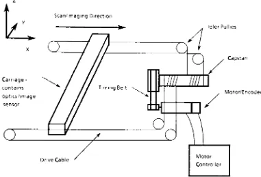
The

physical system under

investigation

is

shown

schematically

in

Figure

1

5.

An

original

is

placed

on

the

platen glass positioned at a

fixed height

in

the

z-direction

above

the

carriage.

The

carriage provides

the

relative

scanning

motion

in

the

xy

plane

between

the

_original

and

the

image

_sensor.

The

motion

is

achieved

by

a

single-capstan

dual-cable

system

(Figure

15).

The

Drive Cable

IdlerPulhes

Capstan

Motor/Encoder

FIGURE

15: Physical System

carriage

rides

on

two

precision-ground carbon steel

shafts

which

are

fixed

to

the

machine

base.

Five

bearing

surfaces support

the

carriage

on

the

shafts.

This

configuration prevents rotation of

the

carriage

about

the y

and

x

axes.

[image:35.523.74.455.214.473.2]

from

the

drive

motor

(4:

1

drive

ratio).

The

feedback device

is

a

1000

lines/rev

incremental encoder.

Two

encoder

outputs,

90

degrees

out

of

phase,

yield a

quadrature

output

of

position

and an effective resolution

of

4000

lines/rev.

A

4-pole

permanent-magnet

DC

motor

is

the

prime mover.

Specifications

for

the

drive

components

and

manufacturer's

literature

_on

the

motor/encoder

package are given

in Appendix

B.

Figure

16

shows a

block diagram

of

the

control and

mechanical

system

interactions.

The

control system produces

the

torque,

Tmot0r,

which

sets

the

mechanical system

in

motion.

The

dynamics

of

the

mechanical system affect

the

motor position

which

is

the

primary feedback

variable.

The

control

Microprocessor

Position Xcarriage

Vcarriage

Acarriage Position _Error

Command

^^-^ Digital

i _PWM

Filter/ i _amplifier/

DtoA

j

Motor Converter i

Circuit

'_motor

Motor/Capstan

Carriage Dynamics

+s

-. _ _ _ J

^motor

Sack EMF

Feedback

Position

^motor

Encoder

[image:36.523.66.475.345.581.2]

hardware

is

based

on

the

Intel

80286

microprocessor

which resides

in

a

personal

computer.

A

prototype expansion

board handles

decoding

of

the

encoder

output,

digital

to

analog

conversion,

control

loop

timing,

and

assigns

communication addresses.

Initialization

of

variables and

generation of

the

position and error commands are encoded

in

software

(C

language). Since

the

position and error commands reside

in software,

an

inherent

flexibility

in

customizing

and

optimizing

these

portions

of

the

control system

is

allowed.

An

external pulse-width modulated amplifier

circuit,

based

upon

the

L298

integrated

circuit,

amplifies

the

error

command

to the

motor.

Operationally,

the

motor

is

commanded

to

ramp up

as shown

in

Figure

17,

Velocity

(m/s)

Velocity

requiredfor 50% magnification

Nominal

Velocity

Velocity

requiredfor 200%magnification

Imagesensor

activated

[image:37.523.50.473.329.587.2]

Time

(seconds)

and must

then

settle

to

an

acceptable

constant

velocity

before

the

image

sensor

is

activated.

The

nominal

velocity

of

the

carriage

depends

upon

the

speed and resolution

of

the

imaging

sensor.

The

nominal

slow-scan

velocity

forthe

scanning

device

is 208

mm/s.

This

corresponds

to

a motor

velocity

of

51

rad/s.

To

provide

for 50

-200%

image

magnification, the

carriage must

be

able

to

scan

one-

half

and

twice

the

_nominal

velocity

(104

and

416

mm/s respectively).

The

motion requirements

during

the

steady-stateor

imaging

portion of

the

IV

MATHEMATICAL

MODELING

For

the

scanning

system

under

consideration, two

distinct

subsystemscan

be

identified.

The

mechanical

subsystem

includes

several elements - scan

carriage, cables,

drive belt

and motor.

The

dynamics

of

these

lumped

elements are

readily

described

by

the

usual

laws

of classical mechanicsand

the

subsequent system

of

differential

equations.

The

control subsystem

elements,

however,

are considered

individually

due

to the

nonlinear

behavior

of

some elements.

Each

function

of

the

control subsystem

is

represented

by

a

block.

By

using

the

appropriate

assumptions,

a

relationship

between

the

input

and

ouput variables of

that

block

can

be

determined.

The

reduction of

the

control system

to

a mathematical model

demands

that

each

element and

its

behaviour be

thoroughly

understood.

This

section

discusses

in

detail

how

the

control and mechanicalsubsytems are modelled.

Controls

Model

The

initial step in mathematically

modeling

the

control nucleus of

the

scanning

system

is

a

more specific

definition

of

its individual

control

elementsMO-14].

Figure 18

elaborates on

the

single-block representation of

the

control system

initially

given

in Figure 16.

Each

block

represents

a

mathematical

relationship

between input

and

outputvariables.

All

variables

depicted

are time-varying.

This

system

has direct digital

control of

the

motor

position,

01,

and provides

the

forcing

function

torque

necessary

for

input

to

the

system of

differential

equations

that

describe

the

dynamics

of

the

mechanical system.

In

turn,

the

dynamics

of

the

mechanical system

affect

the

the

secondary

loop

variable

_of

motor shaft

velocity,G)i

.

The

control system

PC

based

Microprocessor

1 Position 1 _Command ^ e

C>

i i i i up U PD Control Law

Kd

kp

v3

vm

Motor Circuit 1

. 1 ,

-h

DAC PWM

-(!)

+

\

*

'

Ts

1

+

"

vb

BackEMF

!

f Ka

CO,

|

Position ! Feedback Encoder ' _from motor

Ui6

s

4Nenc

e,

[image:40.523.52.475.108.350.2]

\

in

Figure 18:Controls

Block Diagram

consists of

a

digital

section and an

analog

section.

The

microprocessor

samples

the

motorencoder

every

Ts

seconds

(nominally

600psec)

to

obtain

the

position

feedback,

f,

and compares

it

to

a position

command,

c.

The

resulting

discrete

error,

e,

given

by

e =

f-c

(4.1)

isthen

digitally

filtered

using

a proportional

/derivative

(PD)

control

law.

The

discrete

corrected or compensated

error, up,

which

is

output

to the

Digital to

Analog

Converter,

(DAC),

can

be

expressed

using

the

present

value

The

result

is

expressed

as

up

=

Kpek

+_Kd_[ek-ek-i]

(4.2)

Ts

where

Kp

is

the

proportional

gain

constant and

Kd

is

the

derivative

gain

constant.

This

portion

of

the

control system

is

encoded

in

software, thus

the

derivative

and proportional

gain

constants

can

be

adjusted

to

optimize system

performance.

The

discrete

compensated

error,

up,

computed

by

the

microprocessor

every

Ts

seconds

is

then

converted

to

an

analog

signal, u,

by

the

D

to

A

converter,

DAC.

The

modelled

DAC

has

an

eight-bit

resolution

and

maximum output voltage

of

3.3

volts.

Since

it is

a

discrete

device,

the

DAC

can

only

recognize

a

limited

range of

digital input

values

beyond

which

its

output

becomes

saturated.

Thus

the

range of

discrete

compensated error enabled

by

the

DAC is

28/2

or

128

encoder counts.

A

value

above

128or

below-128

will

saturatethe

DAC

and

limit

the

output voltage

to

the

amplifier.

Since

the

D to A

converter

must calculate an

analog

voltage,

a

computational

delay

of

10

microseconds

was

also

included in

the

representation of

this

control element.

Amplification

of

the

analog

error

signal, u,

is

accomplished

by

a

Pulse Width

Modulated

amplifier

(PWM)

with

a

switching

frequency

of

20khz.

This

type

of

amplifier,

as

the

name

suggests,

modulates

the

width of

the

pulse sent

to

the

motor

depending

upon

the

level

of error

between

the

command and

the

feedback.

Appendix

C

explains

the

operation of

this

element

in

more

detail.

The

resulting

ouput,

Va,

is

the

amplified command signal

applied

to the

motor

The

modelling

of

the

permanent

magnet

DC

_motor

requires some

simplifying

assumptionsti

1.15-19];

1

.

Magnetic

fieldflux,cb,

created

by

the

permanent magnets

is

constant.

2.

The

torque

developed

is

proportional

to the

magnetic

field

flux,

cb,

and armature

current,

ia,

given

explicitly

as

Tmotor

=

Ky

dp

ia

(4.3)

3.

Nonlinear

affects,

such

as

torque

ripple

due

to

the

commutation

discrete

poles are

ignored.

4.

Induced

electromotive

force (Back

EMF)

is

proportional

to

motor

shaft

velocity,

an

:

+

a

j>

vm

o--\AAA

Motor

Figure

19: Motor

Circuit

Vb

=

KeG0i

(4.4)

The

voltagewhich acts on

the

motor

armature,

Vm,

is

equal

to the

amplified

command

voltage,

Va,

reduced

by

the

back EMF

voltage,

Vb,

generated

in

the

motor armature.

Thus

The

motor

armature

may be

modelled

as an

R-L

circuit as represented

in

Figure

19

with a

driving

voltage

of

Vm.

The instantaneous

potential

difference

across

the

inductor

is

La

dia

/dt

and

that

across

the

resistor

is

given

by

Rm

'a-

The

sum

of

these

potentials equals

the

applied

voltage

to the

circuit

indicated

by

Ladja

+

Rmia

=

Vm

(4.6)

dt

Assuming

initial

conditions equal

to zero, the

Laplace

transform

ofequation

4.6

results

in:

(LaS

+

Rm)ia(s)

=

Vm

(s)

(4.7)

or rearranging:

LsM.

=

1

(4.8)

Vm

(S)

(La

S +

Rm )

Thus

the

transfer

function

of

the

armature

circuit

is

described

by

a

first

order

pole and

can

be

written

as

ia(s)

=

1

(4.9)

Vm

(s)

Rm

(

xes +

1

)

where

xe

is

the

electrical

time

constant of

the

motor circuit.

Consequently,

the

motor

does

not

immediately

respond

to

an

input

voltage

due

to

armature

lag.

Multiplying

equation

4.9

by

the torque constant,

Kj

, we

arrive at

an

expression

for

the

generated

torque:

Tmntnr(s)

=

_J<I

(4.10)

Vm(s)

Rm(xes+

D

The

effective

motorvoltage

is

the

applied voltage

Va

less

the

voltage

Vm(s)

=

Va(s)

Vb(s)

(4.11)

where

the

back

EMF

voltage can

be

written

as

Vb(s)

=

KeCOi(s)

(4.12)

Thus

generated motor

torque, Tmotor,

in

terms

_of

the

_{applied voltage and}

rotational speed

of

the

motor

is

Tmotor(s)

=

(Va(s)-KpCOi(s))

Kt

(4.13)

Rm(xeS+

1)

Equation

4. 1 3

shows

the

dependence

of motor

torque,

Tmotor,

upon

the

input

voltage,

Va,

and rotational speed

of

the

motor,

coi,

as

well as a

lag

in

response

due

to

the

inductance

of

the

armature

windings.

The

driving

torque,

Tmotor,

is

used as

the

forcing

function

in

the

system of

differential

equations

that

describe

the

mechanical subsystem.

The

last

control

element

to

be discussed

is

the

encoder.

Although

this

element

discretizes

motor

position,

it

was

treated

as

a

constant

-gain amplifier

element.

At

steady

state, the

lowest

velocity

of

the

motor

is

~4rev/sec.

Th

is

corresponds

to

a

sample

rate of

the

motor position at

1

6.4

khz.

The

nominal

sampling

rate of

the

control system

is

1

.67

khz. This

10:1

ratio

is

high

enough

to

prevent

aliasing

of

the

motorposition.

The

physical constants

and

specifications of

the

scanning

system

are

given

in

Simple

Mechanical

Model

Assuming

sufficiently

high

belt

and cable stiffness and

neglecting

carriage

and capstan

dynamics,

the

mechanical

subsystem

may be

represented

by

a

lumped

inertia

at

the

motor shaftHBJ

.

Viscous

and coloumb

friction

_are

the

resistive

forces

present.

Denoting

lm,

B,Tf

and

Tmotor

respectively

as

the

system-reflected

inertia,

damping

coefficient,

frictional

torque

and generated

motor

torque,

the

differential

equation

_of

this

simple mechanical model

reduces

to

lmdco

= _-Bw

Tf

₊

Tmotor

(4.14)

dt

where

a)

is

the

rotational

velocity

of

the

motor.

Combining

the

frictional

and

driving

torque terms in

a

single

term,

TreS/

and

taking

the

Laplace

transform

yields

(lms

+

B)co(s)

=

Tres(s)

(4.15)

from

which

and as a result

co(s)

=

1/(lms

₊

B)

(4.16)

Tres(s)

H(s)

=

coisi

(4.17)

Tres(s)

Thus

the

transfer

function,

H

(s),

of

the

simple mechanical model

is

also

a

first

order

pole

and

can

be

modelled as such.

The

block diagram

of

Figure 20

shows

the

motor

and simple

mechanical

model.

Motor

position

can

be

obtained

by

simply

integrating

the

velocity

term.

This

simple model provides

MS>-

'Tiotor(s' V^(S)

CO,(s>

T(s)

Back EMF

K

CO,

Motor

Position

To Microprocessor

Mechanical

Model

The primary

concern

of

this

investigation

is

the

oscillatory

response

of

the

scanner

in

the

process

direction,

and as

such, the

following

degrees

of

freedom

which are

kinematically

responsible

for

this

_motion

are

taken

into

consideration:

1

.)

Translation

of

the

carriage

in the

_x

direction;

2.)

Rotation

of

the

motor about

the

x

axis;

3.)

Rotation

of

the

capstan about

the

x

axis;

4)Rotation

of

the

carriage about

the

zaxis.

idlerPulhes

Motor/Encoder

Drive Cable Motor

Controller

FIGURE

15: Physical

System

Rotation

of

the

carriage about

the

x or

y

axis and

linear

movement

in

the

z or

y directions is

prohibited

by

a

low-profile

carriage,

proper placement

of

the

[image:47.523.74.452.282.567.2]

to the

guide shafts.

Figure

1 5

is

reproduced

so

the

reader

may

visualize

these

degrees

of

freedom.

In the transition

from

the

physical mechanical

system

to the

mathematical

model,

several

simplifying

assumption are

made:

1.

Natural

frequencies

of

the

idler

pulleys are

high (>

500

hz).

Previous

work

including

these DOF

in

the

model verified

this

assumption.

2. Idler

pulley

masses

are

lumped

with other significant masses:

2

lumped

with capstan mass

/ 4

lumped

with carriage

mass

3.

Rigid

mountings

i.e.

pulley

supports/

brackets

no structural

deformation.

4.

Only

drive-side

springs are

included

5. Capstan /motor

is

constrained

to

rotate about

the

x axis.

6.

Cable

acts as

linear

spring,

regardless of

carriage

position

(

k

measured

at

3

locations

within

5%).

7 Rayleigh

proportional

damping

is

assumed

@

5%,

consistant

throughout the

model

(translational

DOF)

8. Friction

coefficientsare constant

9. The

system

is

a

lumped

parameter

model,

with

sufficient stiffness

in

the

carriage

to

avoid

finite

element analysis.

The lumped

parameter,

mathematical model

for

the

translational

DOF

Timing

Belt

Cable Motor

Carriage

Figure

21

:

Lumped Parameter Mathematical Model

(Translational

DOF)

From the

model

depicted

in Figure

21,

the

equations of motion

forthe

translational

DOF

can

readily

be

obtained[20-22]:

Motor:

MQi

=

Tmotor

-Ri[Ci(RiCO,-R2CO2)

+

Ki(Ri9i

R202 )

]

Tfi

(4.18)

Capstan:

l2d2

=

R2(Ci

(Rico,

R2a)2)

+

K1(Ri0i-R202)l

-Rc[C2(RcO)2-V3) +

K2(RC02-X3)]

Tf2

(4.19)

Carriage

Translation:

M3

a3

=

C2 (Rc"2

_-V3) +

K2

(Rc02

-X3 )

[image:49.523.70.478.93.328.2]

Capstan

Assembly M2

_{c 12}

Motor M

Carriage

Figure

22:

Linearized Lumped

Parameter Model

(all

DOF)

Figure

<