AN APPLICATION OF QUAIDS
Mark Decker
Submitted as part of the requirements for an honours degree in economics at the University of Tasmania.
material that has otherwise been submitted for assessment or publication by myself and
incorporates no copy or paraphrase of any material previously published by any person
I would first like to thank my supervisor, Dr. Ted MacDonald for the time and patience
he has spared me over the semester, and the guidance he has provided when I have
struggled for direction. My gratitude is also extended to Prof. Ranjan Ray, for the
expert assistance he has given me in the use of demand systems, Dr. Rebecca Valenzuela
for her input into the empirical approach the research followed and Ivan Ferko for
computing assistance. A very special thankyou is reserved for Geoff Lancaster, who
graciously assisted whenever asked with data and estimation problems.
To all of you, and the staff of the Economics Department, thankyou.
Finally, I would like to thank my parents, for making my education possible, and
A theoretical model is developed, which resolves the conflict between observed gaming
behaviour and Neoclassical rational agent theory. This model provides testable
hypotheses regarding the participation in various types of gaming activities and the
welfare effects of taxation on gaming.
The demographic and socio-economic determinants of demand for gaming in Australia
are measured using the parametric QUAIDS model. Based on the econometric results,
the regressivity of gaming taxes is calculated using income elasticities of the budget
share of gaming expenditures.
Results obtained provide strong support for the theoretical model, and provide evidence
to support the position that reliance upon gaming taxation receipts by Australian State
C H A P T E R looooooooooooooooooooooooooooooooooooooooooooooooooooooeoooeooooooeoooooooooooooooooooooooooooooooooooooeooo&ooo 1
1. 1 INTRODUCTION ... 1
1. 1. 1 Definition of Gambling and Statement of the Problem ... 1
1.1.2 The Rise of Gambling in Australia ... 2
1.2 RATIONALE FOR INVESTIGATION ... 4
1.3 THE DISTINCTION BETWEEN GAMBLING AND GAMING ... 7
1.4 PLAN OF DISSERTATION ... 9
CHAPTER 2., ... 10
2. 1 THE UTILITY OF GAMBLING ... 10
2.2 TRADITIONAL MODELS OF THE UTILITY OF GAMBLING ... 12
2.2.1 The Psychological Model ... 12
2.2.2 The Friedman-Savage Model.. ... 13
2.3 A REPETITIVE GAMBLING MODEL ... 16
2.4 AN INTRINSIC OR DIRECTLY CONFERRED UTILITY OF GAMBLING APPROACH ... 18
2.4.1 Definitions ... 19
2.4.2 Fair Bet Structure ... 20
2.5 THEFAIRPROSPECTMODEL ... 23
2. 5.1 Treatment of the 'Tiny Utility of Gambling Term' in the FPM ... 23
2.6 THE SMALL GAlv1BLE THEOREM ... 24
2. 7 EXTENSIONS OF THE SMALL GAMBLE THEOREM ... 27
2. 7.1 Multiple Prospects ... 27
2.7.2 Multiple Outcomes ... 27
2.7.3 The Lottery Theorem ... 28
2.7.4 The Unfair Prospect Model ... 28
IMPLICATIONS OF Tiffi SMALL GAMBLE THEOREM ... 29
CHAPTER 3 ... 31
3. 1 EMPIRICAL APPROACHES TO GAMBLING ... 31
3.2 DATA ... 32
3.3 VARIABLES ... 34
3.4 TriEMODEL ... 35
3.4.1 Derivation of the Model ... 35
3.5 EQUIVALENCE SCALES ... 37
3.5.1 Equivalence Scale Model. ... 38
3.6 ESTIMATION ISSUES ... 39
CHAPTER 4 ... 40
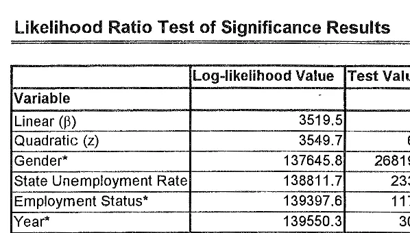
4.1 ESTIMATION ... 40
4.2 THE ECONOMETRIC MODEL ... 41
4.3 RESULTS OF THE DEMOGRAPHIC DEMAND SYSTEM ... 41
5. 1 SUMMARy OF RESULTS ... 48
5.2 LIMITATIONSANDFURTHERRESEARCH ... 48
5.3 CONCLUSION ... 50
APPENDIX leoo••••••••ooooooooooeoeooeoooeoooooeoooooooooooooooooooooooooooooeoeeeooooooooooooooooooooooooooeoooooeoooe 51 THE POPULARITY OF GAMING ACTIVITIES IN AUSTRALIA ... 51
COMPAI<.ISON OF RACING AND GAMING ACTIVITY IN AUSTI<.ALIA ... 51
APPENDIX 2oooooooooeoooooooooooooooooeoooooooooooooooooeoooooooooooooooooo•eooeooooooooooooooooooooee"ooooeoooooeooooo 53 DERIVATION OF TI-IE VARIANCE OF~ ... 53
EVIDENCE FROM PSYCHOLOGICAL TRIALS ... 53
PROOF OF THE SMALL GAMBLE THEOREM ... 54
PROOF OF THE LOTTERY THEOREM ... 57
PROOF OF THE UNFAIR PROSPECT MODEL ... 57
APPENDIX 3oooooooeoooooooooooooooooooooooooooooooooooooooooooooooooooooooooooooooooooooooooooooooeooooooooeeoooooooooo 59 DEPENDENT VARIABLES ... 59
INDEPENDENT VARIABLES ... 59
UNEMPLOYMENT ... 61
REAL PER CAPITA GAMING EXPENDITURE ... 61
APPENDIX 4.o···~~···.,··· 63
INCOME ELATICITIES OF THE BUDGET SHARE OF GAMING ... 63
1.1 Introduction
1.1.1 Definition of Gambling and Statement of the Problem
Gambling has been defined as " ... the wager of any type of item or possession of value
upon a game or event of uncertain outcome in which change, of variable degree,
determine such outcome1 ".
Economics has traditionally devoted little attention to issues involving gambling due to
the difficulty in reconciling the "rational economic agent" and "risk -averse behaviour"
used in expected utility analysis with the actual practice of gambling. The literature has
developed in two main directions in order to reconcile observed behaviour with
economic theory. The participant must either be risk-loving over some section of the
utility function or attain intrinsic utility from the activity.
A theoretical model is developed which illustrates that rational economic agents may
incorporate both gambling and risk-averse behaviour such as insuring, particularly over
some sections of the associated utility function. This theoretical model allows
inferences to be drawn with respect to what factors influence people to gamble, and, in
turn, where the implicit burden of taxation may lie. These inferences are tested
empirically, leading to the formation of the policy implications of gambling.
1.1.2 The Rise of Gambling in Australia
In 1996 Australia had the second highest per capita expenditure on gambling of any
nation, behind only the USA 2 This expansion of the domestic gambling industry has
allowed State governments in Australia to rely relatively more heavily on gambling
revenue when compared to governments in similar economies.3 The 1997 decision of
the High Court of Australia to disallow State governments to continue to levy excise
taxes on petroleum, tobacco and alcohol products implies that this reliance on gambling
revenue to fill State Treasury coffers will continue to grow.
The prevwus decade has seen a significant expansion in State supported gambling
activity in all States, with casinos openmg in Western Australia, South Australia,
Queensland, New South Wales, the Australian Capital Territory and Victoria, as well the
continuing expansion ofTasmania's Wrest Point which opened in 1973 and the Northern
Territory casino. In addition, there has been a notable increase in the number of poker
machines available. State governments, "sensing this relatively electorally painless way
of raising revenue"4, have increased collections of gambling-related revenues. An
example of the effect this has had on State revenues is that in 1996, the $400 billion
Crown Casino complex in Melbourne delivered $1.2 million daily to the State
government in gambling revenue alone. Gambling revenue in Victoria in 1995/96
contributed 12.5% of State own-source revenue, while in Queensland in the same period
the figure was 14.6%5
2 Sixty Minutes, 27/09/97. The real net per capita gaming expenditure for Australians in 1995-96 was
$581.21. 3
Worthington, 1997. 4
Kitchen and Powells, 1991. 5
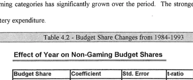
The growth of gambling activity in Australia can be illustrated with reference to annual
aggregate figures published by the Tasmanian Gaming Commission and the Centre for
Regional Economic Analysis (CREA) at the University of Tasmania. Figure 1 presents a
State by State comparison of gambling activitl which illustrates the 300.93% increase
in gambling turnover in the period.
Total Real Gambling Turnover
30000
25000
20000
E 15000
~
10000
5000
0
...-0) 0)
....- ..- .,-- ..- .,... .,... ...- ~
..--""""
Year
In addition it is worth noting that while gaming has remained a popular recreation
activity in Australia the number of persons participating in gaming activity has fallen
from 61.15% in 1984-85 to 55.97% in 1993-94.7 This indicates that the increase in
aggregate gaming turnover results largely from regular participants increasing their
expenditure on gaming rather than an increase in the number of new participants.
6 The period 1984-85 to 1993-94 was chosen to coincide with the period of the Household Expenditure
SutVcy data which will be used for estimation purposes. Figures arc in 1995-96 $A. More detail on this is given in Chapter 3 ..
7 From the HES data. Measured as a percentage of those with some form of gaming expenditure as
1.2 Rationale for Investigation
The expanded reliance on gambling revenues by State governments raises questions as
to the welfare implications of gambling taxes. This leads to two questions for
economists: firstly, what are the determinants of the demand for gambling, and second,
what is the incidence of the economic burden of the implicit gambling taxes. As early as
Pryor (1976), the issue of the regressivity of gambling taxes has been examined. Pryor
found a significant positive relationship between "classical gambling"8 in various
societies and the general socio-economic inequality in those societies.
The majority of gambling-related economic literature has been conducted in the United
States and Canada, and has focused on the regressivity of racing expenditure and State
lottery ticket sales. A notable study by Borg, Mason and Shapiro (1991 )9 is the only
major study to determine demographically the demand for casino games and assess the
incidence of casino taxes in Las Vegas and Atlantic City.10 Using a similar approach,
Scott and Garen (1994) analysed the determinants of demand and incidence of taxation
for the Kentucky State lottery.
Reliance on gambling revenue by State governments has been criticised in the United
States by Madhadhusan11, Suits12, Calmus13 and Stocker14 amongst others and in Canada
8
'Classical gambling' refers to traditional gambling activities such as wagering on horses, card games etc. This excludes lotto style gambling and such modern innovations as poker machines. Due to the increased accessibilty of gambling products to lower socio-economic groups, such a relationship may be negative for some products in Australia.
9
The Incidence of Taxes on Casino Gambling: Exploiting the Tired and Poor.
10
Regressivity in Australia may be more pronounced due to lower cost of access to casinos.
11
Madhadhusan, R., 1996.
12
Suits, D., 1977. 13
by Henriksson15. The focus of this criticism has been the influence of other economic
factors on gambling revenue as well as the potential regressivity of gambling taxes, (see
Suits 1977). This criticism does not appear to have dissuaded either Australian State
governments or US and Canadian governments from following the trend 16 of attempting
to establish a solid revenue base from gambling.
A point of contention in gambling theory is whether or not the sale of gambling products
should be considered as implicit taxation, because the purchase of gambling products is
voluntary. Kitchen and Powells (1991) argue that consumption of such products is "no
different from the consumption of alcohol, tobacco or any other taxed product. Indeed,
the implicit [gambling] tax is exactly analogous to an excise tax on any commodity". 17 A
welfare implication of the consumption of gambling products is that the implicit taxation
may be fundamentally regressive, "that is, the tax paid by households as a percentage of
income is higher for low income households than high income households". 18 Kitchen
and Powells (1991) are supported by Borg, Mason and Shapiro (1993):
" ... taxes on gambling are taxes even though gambling is a voluntary
activity. Specifically, they are excise taxes in the same wcry that
assessments on liquor and cigarettes (two other voluntary purchases) are
taxes. As a result, it is valid to consider whether the burden imposed by
taxes on gambling is distributed in an equitable manner." 19
14
Stocker, F., 1972 15
Henriksson, L., Hardly a Quick Fix, Canadian Public Policy, 22(2) June 1996, 166-28.
16
What Madhadhusan and Hcnriksson term "Casino Fever". 17 Clotfelter and Cook ( 1989), Ch.ll.
1
g Kitchen and Powells (1991), pg 1849. 19 p
This proposition is supported by empirical evidence that gambling is more prevalent in
lower socio-economic households20, thus making a tax on gambling regressive.
This evidence is more strongly supportive of the hypothesis that gaming as opposed to
other forms of gambling21 is regressive:
"On the basis of the sample who have given themselves access to casino
gambling, the tax is regressive; in fact it is extremely regressive in Las
Vegas. Therefore, in this time of easier access to casino gambling,
policy-makers should be aware that the taxes on casino gambling place a
proportionately heavier burden on low income groups. "22
The accessibility of gambling facilities is cited in Borg -et al (1993) as a major factor
influencing the difference in the comparative regressivity of gambling taxes in Las
Vegas, Nevada and Atlantic City, New Jersey. The results from this study show that the
incidence of taxation from the relatively more accessible gambling facilities of Atlantic
City23 is more regressive than the incidence of gambling taxes in Nevada. The
implication to be drawn from this study is that the implicit tax burden has the potential
to be more regressive as gambling facilities become more accessible. This is
particularly relevant in Australia, where the expansion of gambling facilities in all
major cities has made access to such activities easier than in any comparative economy
and at any other period. By supporting the expansion of gambling facilities, State
20
See, for example, Sixty Minutes, 27/09/97 and Bulletin Magazine, 30 July, 1996, and 19 December, 1995.
21
Section 1.3 defines this distinction. 22
Ibid, p 323. 23
governments may be creating a more regressive tax system, particularly with the
observed increases in gambling turnover in each State.
The aim of this paper is to extend the content and quality of the available economic
literature concerning gambling activity in Australian economic research, which at this
point is currently one study: Worthington 1997. The goal is to identify the determinants
of demand for gaming in Australia and measure the regressivity of gaming taxes.
1.3 The Distinction Between Gambling and Gaming
Gaming expenditure is defined as expenditure on "all legal forms of gambling other than
racing, such as lotteries, poker and gambling machines, casino gaming, football pools
and minor gaming (which is the collective name given to raffies, bingo, lucky envelopes
and the like"24. Gambling expenditure is defined as expenditure on gaming plus all
racing expenditure, which "comprises legal betting with bookmakers and totalisators,
both on and off-course (TAB). It is related to betting on the outcome of horse and
greyhound races, and, in recent times, on some other specified sporting events, such as
football matches". 25
24 Tasmanian Gaming Commission and CREA, Australian Gambling Statistics 1972-73 to 1995-96, pg. 2.
25
In this paper a clear distinction will be made between gambling and gaming, as defined
by the Australian Bureau of Statistics26, for two reasons. First, there is significant
anecdotal evidence27 to suggest that racing wagering is more the province of
'high-rollers'; that is, there is a notable socio-economic difference between participants in
racing wagering and gaming activity, with the racing industry enjoying support from
those in a more financially secure position. The second reason is that in all gaming
activities, the price of the game, the 'takeout', is fixed, as are the associated probabilities
of a successful outcome for any wager. Racing expenditure is also pari-mutuel in nature,
meaning that the relative expenditure on each prospect (eg. horse) in each trial (race)
determines the pay-off for a successful wager. Further the probability of being
successful on any wager is not constant, but is also a function of human knowledge and
expertise. That is, knowledge may improve the probability' of success.
Finally, it is worth noting an empirical justification for this distinction. Racing turnover
has been virtually static over the past decade 1984-85 to 1993-94, while garnmg
turnover has increased dramatically, as is illustrated by the tables in Appendix 1.
The focus of the analysis is on estimation of determinants of gaming expenditure within
a fully specified demand system. The aim is to identity the significant demographic
determinants of demand for gaming in Australia and to measure the potential regressivity
of gaming taxes.
26
Gaming is defined as "all legal forms of gambling other than racing, such as lotteries, poker and gambling machines, casino gaming, football pools and minor gmning (which is the collective name given to raffles, bingo, lucky envelopes and the like)".
27
1.4 Plan of Dissertation
Chapter 2 presents a revtew of the existing theoretical literature on the utility for
gambling with an emphasis on the directly conferred utility of gambling, establishing an
approach whereby the observed behaviour of economic agents who both gamble and
insure may be studied within the Neoclassical expected utility maximisation framework.
Chapter 3 discusses the relevant data and estimation issues. Results of the estimation
process and the measures of the regressivity of gaming taxes are presented in Chapter 4.
A summary of the results and policy implications of the estimation, and areas for further
2.1 The Utility of Gambling
There is a comparatively small amount of economic literature devoted to the analysis of
gambling, due in part, to the difficulty in reconciling the activity of gambling with
standard economic analysis. "It is hard to explain why individuals simultaneously pay to
decrease risk [insurance] and pay to increase risk [gambling]"1. The differing behaviour
evidenced by economic agents who both gamble and insure is a puzzle for economists
attempting to explain the incidence of gambling within the neoclassical framework of
expected utility maximisation of rational agents. The standard methodology is to treat
gamblers as having the sole motive of improving their wealth position, 2 the intrinsic
utility to be gained from gambling as a recreation activity "is well recognised, but almost
always resisted"3.
Samuelson (1952) commented that "a large fraction of the sociology of gambling and
risk-taking will never be significantly discernible in terms of money prizes alone, as
distinct from elements of suspense and gamesmanship"4. This view was again voiced by
Becker after the 1977 Survey of American Gambling Attitudes and Behaviour " ... the
activity of gambling rather than the implications for wealth, is the primary motive for
most forms of gambling; and gambling takes place despite substantially unfair odds"5.
1 Conlisk (1993).
2 Since, due to low probabilities of winning, all gamblers will be losers in the long run, this approach
would seem to be flawed, particularly if the neoclassical assumptions of perfect information and rationality apply.
3
Ibid(l993).
4 Samuelson 1962 p 677.
5
This is especially true for gaming, where in repeated plays, the gambler is certain to lose,
but less so for wagering, where through the use of knowledge, certain betting techniques
and human error there is scope to win in the long run.
It is somewhat surprising to find that in the interim period between Samuelson and the
present, economics has developed two fundamentally different models to explain
gambling behaviour, but neither includes any utility of gambling itself. The utility
functions are defined only in terms of the expected payoffs and the probabilities of
winning.
The following sections outline the two traditional models of gambling behaviour, and
then a new approach which incorporates an intrinsic, or directly conferred, utility of
gambling as suggested but not incorporated by Becker (1977), Arrow (1974),
Hirschleifer ( 1966) and Markowitz ( 19 52). The Conlisk ( 1993) model of intrinsic utility
provides a rationale for risk-averse and risk-loving behaviour to exist simultaneously
while maintaining the neoclassical expected utility framework.
This approach is supported by Daniel Suits, a leading US economist in this field, who
argues in favour of gambling directly conferring utility:
"Gambler's are perfectly aware that they will lose on the average, but they
view this expectation of loss as the price paid to engage in the game. For
most gamblers, in other words, the purpose of gambling is not to get rich, but
to 'have fun', to experience 'excitement', or to have 'something to look
others look on outlays for theatre tickets, vacation trips, or a night on the
town." 6
2.2 Traditional Models of the Utility of Gambling
2.2.1 The Psychological Model
The first of the two traditional models is the psychological model, where gambling is
viewed as an enjoyable pastime, participation in which embues the gambler with
personal and social gratification like other recreation activities, but the actual
participation is modelled on the gambler systematically misperceiving the probabilities
involved in risky prospects? Brunk (1981) cites, amongst others, psychological studies
by Preston and Booth (1948), Fellner (1965) and Yaaii (1965), and argues that the
" .. .long history of psychological research investigating individual behaviour under
conditions of risk [as explained above] should be a generally accepted psychological
law"8. Weitzman (1965) and Ali (1977) provide empirical support for the contention
that individuals systematically overestimate beneficial but low probability outcomes
(winning) and underestimate chance of detrimental outcome (losing) as investigated by
Brunk (1981).
6
Suits (1979). 7
The misperception of the odds is what stimulates the actual participation. According to the theory, even though the activity provides utility, rational agents will not participate due to the fact that in the long nm gamblers will worsen their wealth position. Only if the probability of success is favourably misperceived will a gamble be accepted.
2.2.2 The Friedman-Savage Model
The second model is the Friedman-Savage model, named from a seminal 1948 paper, in
which the authors described a utility function that has a shape allowing both risk-loving
and risk-averse behaviour. The model uses an expected utility of wealth function with a
concave central section allowing risk-loving behaviour to be consistent in that area, with
a standard convex shaped utility function across low and high wealth ranges. The
concave section of the expected utility of wealth function explains risk-loving behaviour
such as gambling even when the prospect is unfair, in the sense that the expected payoff
is less than the wager. Absolute wealth and relative wealth positions form the basis of
the utility functions in the majority of the economic literature on the utility of gambling.
Friedman-Savage model is based on a relative wealth structure across individuals, while
the willingness of each individual to gamble is based on the relative wealth position of
the individual.
Participation in the Friedman-Savage model is qualified by what the authors term the
'disaster zone'. A risky bet will not be accepted if, by losing, the gambler will enter an
area of their wealth function which leads to disaster; ie. if this leads to a situation where
financial commitments can no longer be honoured. Kwang's (1965) discontinuous
utility function assists in explaining theoretically why this may occur.9 For example, if L
in Figure 2.1 was below the weekly financial commitments of the gambler, then the bet
would not be taken.
9
U'
Utility
···-~:~··"N···,...
...
....
···
• • • • I
Wealth
This utility function assumes that an individual's expected utility from any given bet is
the probability ofwinning times the utility of his wealth if he wins, plus the probability of
losing times the utility of his wealth if he loses.
Assume initial wealth is Wn. Two bets are examined. The first offers wealth L if the
bettor loses and G if he wins. The weighted utility of these wealth positions lies on LG,
at P, given the assumed odds. Since P is below N, the point on the utility function
corresponding to the initial wealth, the individual will not accept the bet. The second bet
offers wealth L associated with a loss and wealth G' for a win. The weighted utility of
this bet, given the assumed odds, lies along LG', at P', which is above N, implying that
the individual will accept this gamble.
In general terms, the Friedman-Savage model contends that an individual will choose to
game is greater than the utility derived from the present wealth level. Formally
presented, an individual will gamble if and only if:
E(U) =PU(IJ) + ( 1-P )U(/2); where: U is the utility of income;
P is probability of a beneficial outcome;
!1 is income after a favourable outcome;
and; 12 is income after a negative outcome.
Brunk ( 1981) provides empirical support for this model. Based on survey answers to
the question "Are you satisfied with your present income?", results indicate that across
the seven categories of satisfaction, those that were most dissatisfied spent an average of
$56.21 more per year on lotteries than the most satisfied.10 Further work on the
Friedman-Savage model has been conducted by Markowitz (1952), Kwang (1965),
Tversky (1967) and Pryor (1976). Markowitz illustrated that the UU' curve in the
Friedman-Savage model gave a number of paradoxical results, and eliminated these by
slight adjustments to the UU' curve11. Kwang (1965) reinstated the traditional
decreasing marginal utility of wealth assumption by making the function UU'
discontinuous at the current wealth position. This was justified on the basis that this
modification by arguing that gambling behaviour is defined by the indivisibility of the
cost of purchasing a good.12 Beneficial outcomes allow the bettor an opportunity to
purchase goods that are otherwise outside the wealth range of the bettor, while a
non-beneficial outcome will not shift the wealth position of the gambler to such an extent
that the 'disaster zone' phenomena ofthe Friedman-Savage model operates.
10
This is a close proxy for the Friedman-Savage premise that dissatisfaction with income is the motivating factor behind people gaming.
11
2.3 A Repetitive Gambling Model
Lee (1969) extended the Markowitz model by incorporating the possibility of repetitive
playing. Gambling activity is undertaken due to the utility derived from a change in
wealth, but this is determined by the outcome of previous wagers as well as the present
result. The importance of this study is that it was the first to formally recognise that
gaming, such as craps, poker machines, blackjack and keno, is conducive to repetitive
play.
The repetitive gambling framework is based on the expected change in wealth per play:
PI L1 WI +
p2
L1w2
= L1w;
where: PI is probability of winning;P2 is probability of losing;
L1 WI is change in wealth if win;
L1
w2
is change in wealth if lose;From the Friedman-Savage model, an individual will take the prospect13 if the expected
utility of playing the game is greater than the expected utility if the game is not played,
ie. the utility of the present wealth level:
(2.1)
In a repeated game, the player will therefore take the prospect if his expected utility of
the change in wealth per play of the game is greater than zero. However, since the
expected change in wealth is known, should the prospect be taken, the expected utility
12
of the change in wealth associated with playing a repeated game once is dependent upon
the previous outcome. That is, the gain in wealth L1W1 or the loss L1W2, resulting from
the previous playing of the game, are directly related to the size of the gain or loss in the
subsequent outcome of the gamble. The variance of LiW resulting from playing the
game once is also directly related to the previous outcome, since individuals update
expected variance by the previous result.
Allowing
x;
to be a random variable representing LiW from the first trial;Var(XJ = E(X/ - E(X/
For a derivation of the variance see Appendix 2.
(2.2)
If the game is repeated n times, where each repeat 1s an independent trial with a
stationary mean and variance, LiW per play becomes:
1 n 1 2
var (-
Z:x;J
= -PrP2
[~fr;- A~]n i=l n
(2.3)
while the expected change in wealth remains:
E(X;)= ~W14 (2.4)
Substituting these values into the expected utility equation yields:
This inequality must be satisfied if the prospective gambler is to play the game.
13
In this chapter the terms "gamble" and "prospect" are used interchangeably. A technical distinction may be drawn between the two in that a gamble, by definition, involves a risk, whereas a prospect does not necessarily have such a characteristic. Hence a gamble may be called a "risky prospect."
14 E(_!_
fx;)
=
_!_nE(X;)=
E(x;)=
AWHowever, this model relies only on P and L1W in order to come to this conclusion. Since
Lee does not make an attempt to reject the psychological model the misperception of
odds may therefore influence the number of gamblers who will play the game and the
number of repetitions each gambler will undertake.
The criticism of the traditional models of the utility of gambling above and the
subsequent research is that "Economists have resisted the idea of a utility of gambling15"
in the sense of an intrinsic utility such as the "suspense and gamesmanship" of
Samuelson (1952). By developing a model that does allow for a directly conferred
utility of gambling to exist the apparent contradiction of a rational economic agent both
insuring and gambling may be explained.
2.4 An Intrinsic or Directly Conferred Utility of Gambling Approach
Conlisk (1993) presented the "Tiny Utility of Gambling Model" which reconciles both
risk-loving behaviour (gambling), and risk-averse behaviour (insuring) as observed to
exist in rational economic agents. The model uses standard expected utility analysis for
a risk-averse model but with a tiny utility of gambling term attached, that reflects the
intrinsic utility to be derived from gambling. This additional term influences choice
between two risky prospects, a risky prospect and a 'sure thing' and whether to take a
risky prospect or not. The term influences choice since it adds a positively signed term
to the usual expected return structure, making it more likely that a prospect will be
accepted.
15
The model predicts that a variety of small gambles will be accepted by risk-averse
economic agents but remains consistent with behaviour observed by individuals facing
large risks. In contrast to Friedman and Savage (1948), Markowitz (1952), Kahneman
and Tversky (1979, 1986, 1991) and Machina (1981,1987) the Small Gamble Theorem
developed by Conlisk allows for simultaneous gambling and insuring for any probability
of winning and associated gain or loss, that is, for any risk-return structure of a gamble,
providing an improvement upon the previous models which only allowed such a range of
behaviour over severely restricted pay-off structures. Conlisk also supports the
proposition of Markowitz (1952) and Lee (1961) that an individual's objective function
is concerned with the potential change in wealth rather than absolute wealth positions.
2.4.1 Definitions
A fair bet is any gamble for which the expected returnpG + (1-p)L = 0; a risky prospect
is any gamble where the probability of an unsuccessful outcome, (1-p), is greater than
zero. That is, there is a positive probability oflosing.
A fair prospect is any gamble which offers a fair bet structure as outlined above. Note: a
fair prospect may be risky, although, unlike a gamble, a prospect is not constrained such
2.4.2 Fair Bet Structure
Assume a fair bet where G is the gain from a successful outcome and L is the loss from
an unsuccessful outcome of a gamble16:
:. P(G) = p; and; P(L) (1-p).
A fair bet for a risky prospect is: pG- (1-p)L = 0
:.L = pG/(1-p) p = LI(L+G) or p
=
ll[l+(G/L)} (2.6)This can be interpreted as a monotonic function of the gain-loss ratio and is therefore a
measure of the skewness of the prospect, where G is the size of the prospect and p is the
skewness. If an individual accepts the fair prospect (G,p) above then the preference
value becomes an expected utility function modified to allow for the utility of gambling;
E(G,p,K) = pU[K+G} + (J-p)U[K-pG(J-pf1} + eV(G,p); (2.7)
where: K is initial wealth;
U(W) denotes a utility of wealth function which displays
the following characteristics;
U(O) = 0; U'(W)
>
0, U"(W) < 0;and; U(W) < Uw
<co;
Wealth= K +G with probability p;
=
K-L=
K-pG(J-p/1 with probability (1-p);and; sV(G,p) is the intrinsic utility of gambling17.
:. A risky prospect (even a fair bet) will be accepted if and only if:
E(G,p,K) > E(O, O,K) = U(K). (2.8)
16
For the purpose of the Fair Bet Structure it is irrelevant whether G and L are absolute values (as is usually the case with gambles) or arc relative to initial wealth.
17
V(G,p) is the utility gained from the excitement and suspense the individual feels in the
period between the acceptance of the prospect and the resolution of the uncertainty and
8 is the utility of gambling independent of the potential gain and the probability of a
successful outcome. Note that this is the utility derived from anticipating a successful
outcome and associated improvement in the wealth position of the gambler, and is
dependent on the risk-return structure of the prospect. 8 is determined solely by
individual tastes and it is the utility obtained directly from participation in the gambling
activity, and is therefore independent of the expected pay-off.
Pollatsek and Tversky (1970) derived the standard deviation of a fair prospect, a(G,p),
as representing the dispersion18 of the prospect. Conlisk (1993) extends this theory using
the tiny utility of gambling term, sV(G,p), by specifying V(G,p) to be a function of the
standard deviation:
V(G,p) 19
=
V'[a(G,p)]; (2.9)where a(G,p) is a measure of gambling excitement.20
Therefore, the standard deviation of a prospect may be written as:
a(G,p) = G[p/(1-p)/·5; (2.10)
and the expected absolute deviation may be written as;
a(G,p) = pG = GLI(G+L). 21 (2.11)
18
The dispersion of the prospect is the range of possible retnrns from the gamble around the expected pay-off.
19 For any O<p<l (ie. for a given GIL ratio) it is assumed that V(G,p) as a function of G passes through
the origin [V(G, 0) = 0}, is increasing in G [VJ(G,p) > OJ and is concave [V11(G,p) < 0]. If G > 0 then
V(G,p) increases from zero proportionately with p and :.V(G, 0) = 0 and V2(G, 0) > 0 \7 G > 0.
20 V'[a(G,p)] is a concave and bounded function which converts the excitement of gambling, in the sense of Samuelson's "suspense and gamesmanship' into a utility function.
21
See Pollatsek and Tversky (1970) for a full derivation of these. Note that G[p/(l-p)f5 and
GLI(G+L) are constant elasticities of substitution functions of G and L with 17 = 0.5 and 1 respectively.
This effectively allows Conlisk to avoid the misperception of odds criticism from this
model; the implication is that the odds are not misperceived, rather, the individual
receives greater pleasure per unit from anticipating the expected gain, pG, than
displeasure per unit from anticipating the expected loss, (1-p)L. Therefore utility is
discontinuous at the initial wealth point for each gamble, as in Kwang (1965).
Assigning arbitrary weights of (1 +A,) and -1 to the utility of anticipating winning and
losing respectively yields, where A,
>
0:(J+J,)pG- (1-p)L = J,pG; where A;pG is net pleasure. 22 (2.12)
The change from p to (1 + J,)p improves the gamble expectation of a fair prospect from
zero to J,pG/(1-p), which implies that a(G,p) = pG/(1-p). Since this is not a true belief,
the distortion of the gain probability will occur only in the V(G,p) component of the tiny
utility of gambling term in the utility function and not in the expected utility terms. This
may explain why apparently risk-averse economic agents gamble.
2.5 The Fair Prospect Model.
From the utility function defined in the previous section, the Fair Prospect Model (FPM)
can be derived:
E(G,p,K) =pU[K+G} + (J-p)UfK-pG(J-pf1} + cV(G,p); (2.13)
CJ(G,p) = GaL(l-aJ = (GLf5(G!L/a-o.s) = G[p/(1-p)f!·'l).
Therefore excitement may be increasing or decreasing in the skewness of the prospect, depending on the sign of (a-0.5). Luce (1980, 1981) dicusses four measures of risk. The favoured approach is:
CJ(G,p) = G0p0/A +B(l-p/'0/.
22
where: L = pG/(1-p) .SK (no negative wealth).
The functions in U and V are assumed to be differentiable and obey the following
conditions for any positive K, G and p:
for p < 1: 0 ~~ U(O)
<
U(K)<
Uw<co;
U'(K) > 0, U"(K) < 0.
0 = V(O,p) V(G,O) < V(G,p) < Vw <
co;
VI(G,p)
>
0, V11(G,p) < 0, V2(G,O)>
0.Hence, an individual will accept the risky prospect if and only if:
E(G,p,K) ~ U(K). (2.14)
2.5.1 Treatment of the 'Tiny Utility of Gambling Term' in the FPM
There are two approaches to the treatment of the tiny utility of gambling term for any
particular risky prospect. The first is to assume that the gambling term is present in
gambles, such as wagering on a card game, but not present in non-gambles, such as
purchasing insurance. The weakness of this approach is that classification of prospects
as gambles or non-gambles may be arbitrary.
The second approach is to assume the gambling term is always present, but its effect
may be overborne by the risk-averse expected utility terms.23 Studies provide evidence
that the size of the prospect determines the level of risk-aversion exhibited by
23
individuals24, and the utility of gambling term dominates for relatively small prospects
(no risk of negative wealth if the outcome is negative) but is overwhelmed by the
expected utility terms when the stakes are large. The main advantage of this model is
that the theorems provide testable implications without the need to categorise a prospect
as either a gamble or non-gamble.
2.6 The Small Gamble Theorem
For any fair and risky prospect to be accepted under the FPM, the utility of gambling
motive must be greater than the risk -aversion motive, otherwise risk -aversion implies
rejection of any risky prospect.25 Theory therefore requires the weights on the utility of
gambling term to reach some threshold size26 before any risky prospect would be
accepted.
In contrast, the SGT states that any &
>
0 will be enough to make some prospects, asfunctions of (G,p) acceptable, dependent on the risk-return structure.27 The justification
of the SGT and 'tiny' utility of gambling term is that an individual's utility of wealth
function is approximately linear over a small region. This 'local risk neutrality' makes
the risk-aversion motive second-order small, whereas the utility of gambling is
first-order small. 28
24
See Appendix 2 for this evidence. 25
That is c:V(G,p) > pU[K+G} + (1-p)U[K+G(J-pfj
26
The threshold size is theoretically be determined by the risk-return stmcture (G,p) of the gamble. The size of the gamble, or potential loss, would be the cmcial factor, due to the Friedman-Savage
'disaster zone'. 27
E(G,p,K) = pU[K +G] + (1-p)UfK +G(l-pfj + sV(G,p) is always positive under the SGT for small
prospects. This implies that c:V(G,p) > pU[K+G] + (l-p)U[K+G(l-p)"1] and hence the gamble will be accepted.
28
Formally, the net benefit, b(G), from accepting a fair but risky prospect may be
represented as:
b(G)
==
E(G,p,K) - U(K); where p is fixed. (2.15)=>
b(O) = 0;=>
b '(0) c:VJ(O,p);=>
b "(0) = p(l-pl U"(K) + sVu(O,p);=>
b "(G) = pU"(K +G) + p2(1-pl1 U"[K-pG(l-p/1} + c:Vn(G,p). (2.16)All three right hand side terms of b ''(G) are negative and hence b(G) is concave due to
the concavity of both the utility of wealth function, U(W), and the utility of gambling
function, V(G,p)?9
The SGT is concerned only with risky prospects of small size, ie. G is small. As G
increases, the concavity effect will dominate. From (2.16):
b "(G)< 0 \fG; (2.17)
b(G)
m(K)'
8large
8 small
c(K)'
G
29 The SGT rejects the usual association of concavity and risk rejection due to the weight of the utility
and we expect b(G) to rise into the first quadrant as in Figure 2.2, reach a maximum {at
m(K)} and then cross into the fourth quadrant {at c(K)}, if E is not too large. The
subjective weighting E determines the maximum point and the point of intersection
between b(G) and the horizontal axis. The more utility an individual derives from
gambling, the higher will be the maximum, and the further along the G axis will the point
of intersection. 30 This also implies that an individual with a higher subjective weight E
will accept 'less fair' prospects, ie. a prosp~ct where the probability, p, is smaller for the
same return, G.
For values of G greater than c(K) the prospect is unacceptable; to the right of m(K) the
condition of concavity imposed by the expected utility terms in the FGT begins to
dominate. This implies consistency between risk-averse behaviour for large prospects
and gambling.
2. 7 Extensions of the Small Gamble Theorem.
2.7.1 Multiple Prospects
The SGT can be extended to hold for multiple prospects. The individual simply selects
the option with the largest expected utility, E(G,p,K), or will remain at the status quo,
U(K). This analysis is valid for repeated gambling behaviour.
30
2.7.2 Multiple Outcomes
The SGT also holds for prospects with multiple outcomes such as a fair multiple
outcome lottery, which can be represented by a vector of pay-offs, and associated
probabilities:
X=[X};
such that;
and; P = [pJ;
IipX = 0; and; E(p,X,K) = EipiU(K+XJ + sV(X,p). (2.18)
If the ratios among the pay-offs,
X,
are fixed and the probabilities, pi, are fixed then theprospect will be accepted for small
X;
following the SGT. This equation is outside thestandard class of expected utility models because it is non-linear in Pi· 31
2. 7.3 The Lottery Theorem
Another extension is the Lottery Theorem (L T). A lottery offers a large potential gain,
G, but since the probability of winning, p, is very small, the expected pay-off, pG, and
hence the price of a lottery ticket is small relative to other forms of gambling. This
smallness in the expected return suggests that the SGT applies to lotteries. Therefore, a
negative shift in the bettor's wealth position will remain within the locally risk -neutral
section of the individual's utility function. This suggests that the L T is plausible because
it intuitively follows from the mathematical derivation that there exists a range of
for skewness, an extreme lottery will not only be preferred to no gamble, but will be
preferred to other gambles with smaller G-values. 32
2. 7.4 The Unfair Prospect Model
Since all games with a set takeout rate are 'unfair' in that the expected return is less than
the size of the gamble the extension that is the most relevant to gaming, is the Unfair
Prospect Model (UPM). The UPM is essentially the same as the FPM but the
acceptance function now becomes:
E(G,p,K) - U(K)
>
0. (2.19)As long as the takeout rate is sufficiently small, or the weight a on the gambling term in
the expected utility function is large enough, the function will hold. Since the size of s is
determined entirely by individual preferences, there is no extension to the model which
will be consistent across all individuals, but a simple extension is presented in Appendix
2.
2.8 Implications of the Small Gamble Theorem
By defining two different sources of directly conferred utility from the activity of
gambling, one dependent upon the risk-return structure and so related to the excitement
of anticipating a change in wealth, and the second defined solely by individual
preferences, the SGT remains within standard neoclassical expected utility theory.
31
Sec Machina (1982, 1987) for a derivation of the condition and an explanation of non-linear framework. Machina defines a 'local utility function' whose second derivative defines acceptance or rejection. This restores the usual association of concavity and risk rejection.
Unlike previous theories, the SGT manages to reconcile the observed occurrence in
rational economic agents of both risk-averse practices, such as insuring, and risk-loving
behaviour such as gambling. By allowing the size of the gamble as well as the
probability of success to influence the utility function V[G,p
1
inferences may be drawn as to the characteristics of participants in various gambling activities.The implication from the intrinsic utility of gambling function structure is that different
combinations of p and G, which give the same expected return, will influence the
subjective utility derived from a gamble, as well as the individual degree of risk-aversion.
Hence the composition of the risk-return structure will have a causal influence on which
gamblers play which game, even if the prospective bettor is in the locally risk-neutral
section of the utility function. If the expected return is held constant, inferentially one
could expect gamblers with a lower initial wealth position to be attracted to gambles
composed of smaller probability of success, but which offer large gains. In contrast,
wealthier gamblers could be expected to participate to a large extent in games which
offer a higher probability of success, but with smaller gains to be made.
Intuitively this is logical: more wealthy gamblers would appear to have a relatively
higher subjective weight, c:, while those with less initial wealth are influenced to gamble
more by the anticipation of a significant positive shift in their wealth position and hence
the majority of the intrinsic utility of gambling for these bettor's is derived from the
VfG,p
1
function. This postulate is the motivation for the empirical aspect of this paper.It is an a priori expectation that income will influence the type of gaming activity
This implication is supported by the figures in Table 2.1 below, which clearly shows the
fall in lottery expenditure as income rises suggesting lotteries to be an inferior good.
Hansen (1995) found a similar result for the Colorado state lottery in the United States.
Gaming Type
Gaming as income Lotteries Pokies Casino-type Equivalent income
share
Lower Quintile 0.012679 0.001305 0.00367 163.8935
Second Quintile 0.008224 0.00154 0.002923 316.2901
Central Quintile 0.006631 0.001288 0.001027 470.2021
Fourth Quintile 0.004998 0.000953 0.001343 739.9138
Upper Quintile 0.002489 0.000803 -0.00038 1447.336
Casino type games and poker machines do not have such a clearly defined income
pattern, although the general trend for electronic gaming machines is similar to lotteries,
3.1 Empirical Approaches to Gambling
The bulk of the existing empirical studies of gambling activity has been concerned with
greyhound and horse racing. Literature focusing on gaming has generally studied lottery
sales 1, although Worthington (1997) analyses all forms of legal gambling in Queensland
and Borg et al ( 1991) study the incidence of casino-related gaming taxes. The approach
often adopted in modeling the demand for gaming is to estimate either linear2 or
log-linear3 single equation OLS or Tobit demand functions.4 Single equation models of
demand are not able to exploit the restrictions economic theory provide5, and in
particular are unable to investigate the substitution between individual commodity
demands. This paper is the first in Australia to use a systems approach in order to
measure these effects in relation to gaming.
Since the 234.74% growth in real gaming expenditure in Australia over the period
1984-8 5 to 1993-94 has far outstripped growth in national income, it is important to
determine which goods consumers are substituting away from in order to inject a higher
share of their budget into gaming. This approach may also provide some insight into the
relative regressivity of gaming taxes, by comparing the levels of taxes on the goods
substituted on which consumers now spend less and gaming taxes.
1 Eg. Hansen (1995), Scott and Garen (1994), Theil (1991), Kitchen and Powell (1991), Clotfelter and
Cook (1989), Borg and Mason (1988) and Spiro (1981).
2 Eg., Hansen (1995).
3
Borg, Mason and Shapiro (1991).
4
3.2 Data
The data used is pooled Household Expenditure Survey (HES) data from 1984 and
1993. This allows changes in consumption patterns over the period to be analysed. 6 The
1984 survey consists of 4492 households, while the 1993 survey is based on 8389
households, in two levels of records. The first level describes demographic, expenditure
and income information pertaining to each household. The second level details weekly
expenditure on individual commodities. While the 1993 HES survey offers unit record
data, household information is used in order to maintain consistency with 1984. The
reference person for demographic information such as gender, employment status and
country of birth is the household head.
The differing methods of categorising demographic variables in the two surveys posed
some difficulties for consistency, 7 but only marital status and occupation of the
household head were so cross-categorised as to be unusable. 8 Aggregating categories
would not have been effective due to the inclusion of similar groups of workers in
different categories in 1993 when compared with 1984. Gaming data is disaggregated
into six net expenditure categories in the HES.9 Two categories have been aggregated
in order to align the HES data with the minor gaming category defined by the Tasmanian
Gaming Commission and CREA aggregate statistics. The demand system used for
estimation includes three gaming budget shares as dependent variables. These
5 These restrictions are: (1) adding up ie.
I:wi = 1; (2) homogeneity; (3) symmetry and; (4) negativity. These restrictions are further discussed in Chapter 4.
6 1988 is not used due to the lack of a State identifier.
7 The definitions of all variables in the demand system are given in Appendix 3. 8
groupmgs were determined by the risk-return structure of the types of gaming, as
argued theoretically in Chapter 2 and the six HES categories were aggregated to three in
line with the risk-return structure argument. The three categories are: (i) ga which
includes games with a low price, very low probability of winning and a large potential
gain; (ii) gb which is poker machines, offering an intermediate risk-return structure and
are arguably the gaming type most suited to repetitive play; and (iii) gc which includes
casino-type games and such games as keno and bingo which have a higher probability of
success but with smaller potential gains, for the same price as ga.
The two main problems presented by the use of gaming data in estimation procedures is
the presence of negative consumption expenditures (the presence of net winners10) and
the presence of a large number of zero expenditures. 11
The large number of zero expenditures suggests that one possible approach is Tobit
estimation. This process allows the grouping of the sample into non-participants (those
with zero expenditure) and participants (those with non-zero, usually positive,
expenditure). This approach assumes all zeros to be non-participants. This is justified in
part by the extremely small probability of 'breaking even' when gaming, particularly in
any sample week. Use of Tobit estimation accounts for both the influence of various
explanatory variables on the decision, firstly, whether or not to purchase gaming
products, and if the decision is to participate, then secondly, the subsequent decision
regarding how much to spend.
10
The three categories had different percentages of net winners: ga = 2.958%, gb = 1.133% and gc =
1.087<%.
11 The zeros cannot be distinguished into those that had no expenditure and those that 'broke even'.
Although the likelihood of zero expenditure on gaming indicating breaking even rather
than non-participation is very small, the lack of an identifier suggests the approach
followed in this paper, which is to remove the negative values as outliers and treat the
zeros as actual zero expenditure rather than non-participation. Since participation in
gaming is defined by a utility function which is in part determined by the anticipated
utility of success, 12 it is sufficient that participants are aware that some gamblers will
win, because the stake is placed ex ante rather than ex post.
3.3 Variables
A demand system motivated by the theoretical structure developed in Chapter 2 is tested
using a number of socioeconomic and demographic variab1es that have been identified as
significant in previous studies, or that the theoretical structure indicates may have a
significant influence on gaming behaviour.13 Due to the exploratory nature of this paper,
there is no unequivocal a priori rationale for predicting the direction and statistical
significance of many of the regressors. Inclusion of these is justified on the grounds that
results of the impact of household characteristics on gaming expenditure may be useful
for policy makers and other interest groups.
Definitions of all the variables are available from the HES survey material. An
explanation of how the variables have been structured in order to be used in the
estimation procedure is contained in Appendix 3.
12 See Section 2.4.1 for the definition of directly conferred gaming utility.
13 The influence of demographic variables may impact through the arbitrary s term, the level of
3.4 The Model
A parametric demand system for gaming products and other household expenditures is
developed. Existing studies in applied demand analysis commonly use the PIGLOG
model or the Almost Ideal Demand System (AIDS) developed by Deaton and
Muellbauer (1980). These models are rank 2, having budget share equations which are
linear functions of the logarithm of income. Lewbel (1991) shows that US and UK
household consumption data appears to be rank 3, meaning linear Engel curves derived
from the rank 2 models lack sufficient flexibility to model the variety of shapes that
Engel curves derived from household expenditure data, such as that used in this study,
may encompass. 14 Banks, Blundell and Lewbel ( 1993) derived a class of quadratic
logarithmic preferences that provide integrable demand· systems and which are data
coherent. The rank 3 Quadratic Almost Ideal Demand System (QUAIDS) is a simple
generalisation of the AIDS model, but which allows the flexibility of non-linear Engel
curves while retaining integrability.
3.4.1 Derivation of the Model
Defining functions a(p), b(p) and A,(p) as specific functional forms of the first derivatives
of a PIGLOG expenditure function with p being price of the good: 15
a(p)
=
a0 +Las logp,+
L LYsr logps logp, I 2; (3 .1)14
Deaton and Muellbauer (1980) do note that cross-section data often has non-linear Engel curves (at pg. 317) but do not develop a rank 3 model in order to take account of this.
15 The PIGLOG expenditure function is derived from a specific class of preferences which permit exact
(3.2)
log/L(p)
=
LIL)ogp •. (3.3)8
for some constants ao, as, f3s, Yrs and lvs, \:.1 r and s. 16
This implies the QUAIDS model has the indirect utility function for a utility maximising
consumer:
logl(p, x)
= { [
b(p]
}-I;
where xis total expenditure. (3.4)log )la(p) -IL(p)
By Roy's Identity we can obtain the demand for each good, which take the form of
quadratic budget shares:
where: w. =
Y.PYx;
which is the budget share of goods, wherey is income; andb(p)=
IlPA.
(3.6)In order to maintain consistency with economic theory, the parameters should satisfy the
restrictions for:
(a) homogeneity: LYsr
=
0 \:.1 r; (3.7)(b) adding-up: (3.8)
(c) symmetry: Ysr
=
Y rs \:.1 r,s. (3.9)16
In practice, the adding-up restrictions are imposed by dropping a budget share equation
from the demand system when estimating.
Since prices (the takeout rate) of the gaming products has been approximately constant
over the two pooled samples, or present in only one sample, there is no intertemporal
change, and so prices are assumed to be constant and equal to 1. Therefore, we write
the QUAIDS model as:
(3 .1 0)
3.5 Equivalence Scales
Data on household expenditure is "widely acknowledged to provide superior quality
data and a rich source of information on household behaviour and welfare"17
. However,
when using household level data rather than personal unit record data, the impact on the
behaviour of the household composition must be taken into account. This is particularly
relevant when the heterogeneity of family and household structures in Australia is
considered. The differing needs of adults and children influence the expenditure of the
household, and this influence is captured in estimation by the use of an equivalence
scale.
Equivalence scales offer a means to assess what expenditure different household
compositions must have in order to achieve the same level of welfare as the reference
household. The Engel and Rothbarth models are not derived directly from utility theory
17
and rely on stringent assumptions regarding the link between adult welfare and
behaviour. The Engel (1895) model is derived from the theory that the welfare of
households is inversely related to the household budget share of food. The Rothbarth
(1943) scale is derived from the ratio of aggregate expenditures of demographically
different households that maintain constant expenditure on defined 'adult goods'.
Barten (1964) introduced estimation of equivalence scales from systems of demand
functions that satisfy the 'adding up' constraint. Blacklow ( 1997) 18 estimated
equivalence scales using the QUAIDS model for the data which is used in this analysis.
Hence the Blacklow (1997) estimates of equivalence scales for Australian household
expenditure data are used in the estimation, although an average across categories of the
different age and sex categories of dependents in the household is used.
3.5.1 Equivalence Scale Model
The functional form of the model is the QUAIDS model with constant prices can be
expanded to incorporate equivalence scales as follows:
(3.11)
where: m0 = (1
+
KK +¢A)/zAP ; K =number of children in the household; (3.12)and; A
=
number of adults in the household.18 University of Tasmania Ph. D. dissertation, yet to be released. In contrast to the Engel and
Following the Engel method, the scale is normalised at unity for a reference household,
which is assumed to be a childless couple in this paper.
3.6 Estimation Issues
Demand systems are estimated using Maximum Likelihood Estimation (MLE). The
adding up property of demand systems ensures that the sum of the disturbance terms
over each equation within the system will equal zero for each time period. Denoting the
vector of disturbance terms for each time period as Vt, it follows that the matrix of
disturbance terms:
(3.13)
Omitting the final element of Vt, and denoting the resulting sub-vector as v /, and
assummg v t n to be identically and independently distributed, permits the likelihood
function to be written as:
(3 .14)
Heteroskedasticity is tested for and corrected within ShazamE by usmg the HET
command, which uses an information inverse matrix.