Systematic review of the impact of emissions from aviation on current and future climate

Systematic review of the impact

of emissions from aviation on

current and future climate

A technical report by the University of Southampton

Greener

Systematic review of the impact of emissions

from aviation on current and future climate

Authors *Takeda, K; †Takeda, A.L; †Bryant, J; †Clegg, AC

Produced by *School of Engineering Sciences, University of Southampton; †_{Southampton Health Technology Assessments Centre,}

University of Southampton

Correspondence to Dr Kenji Takeda

School of Engineering Sciences Tizard Building

University of Southampton University Road

Southampton SO17 1BJ

Tel: 023 8059 4467 Fax: 023 8059 3058 email: ktakeda@soton.ac.uk

Date completed September 2007

Report reference School of Engineering Sciences Aerospace Engineering AFM Technical Reports, AFM 07/08

Contributions of authors

Development of protocol K Takeda, A Takeda, J Bryant, A Clegg

Background K Takeda

Literature searching IRC, A Takeda, K Takeda

Inclusion screening K Takeda, A Takeda, J Bryant, A Clegg

Data extraction / critical appraisal K Takeda, A Takeda

Drafting of report K Takeda, A Takeda

IRC = information resources centre, Wessex Institute for Health Research and Development

Conflicts of interest None declared.

Source of funding

This report was partly funded by the Royal Aeronautical Society.

Acknowledgements

We are grateful to staff of the Greener By Design team for assistance with the initial stages of this project, and to Karen Welch at the Wessex Institute for Health Research and Development for assistance with the searches. We would also like to thank Dr John Green and Professor Hugh Sommerville for helping to develop the protocol.

This report should be cited as follows:

EXECUTIVE SUMMARY

Aviation emissions have an impact on the global climate, and this is consequently an active area of research worldwide. By adapting replicable and transparent systematic review methods from the field of evidence-based medicine, we aim to synthesise available data on the effects of aviation emissions on climate. From these data, we aim to calculate lower and upper bounds for estimates of the effect of aviation on climate in an objective manner.

For the systematic review an appropriate protocol was developed and applied by two independent reviewers, to identify research that met the inclusion criteria. These included all aviation types, original research studies, climate models with aviation as a specific component, with outcomes for emissions, radiative forcing, global warming potential and/or surface temperature changes. These studies were prioritised and data extracted using a standard process. The 35 studies reviewed here reported radiative forcing, global warming potential and/or temperature changes as outcomes, allowing direct comparisons to be made.

Tabulated results and a narrative commentary were provided for overall effects on climate, and the individual effects of carbon dioxide, water, contrails, cirrus clouds, ozone, nitrogen oxides, methane, soot and sulphur oxides. Lower and upper bounds for these effects, and their relative contributions compared to overall radiative forcing and surface temperature changes, have been described.

This review shows that the most recent estimates for the contribution of aviation to global climate are highly dependent on the level of scientific understanding and modelling, and predicted scenarios for social and economic growth. Estimates for the future contribution of aviation to global radiative forcing in 2015 range from 5.31% to 8.04%. For 2050 the estimates have a wider spread, from 2.12% to 17.33%, the latter being for the most extreme technology and growth scenario. These global estimates should be considered within the context of uncertainties in accounting for the direct and indirect effects of different contributions. Variations between lower and upper bounds for estimates of radiative forcing are relatively low for carbon dioxide, around 131%, to 800% for cirrus clouds effects, and 1044% for soot. Advances in climate research, particularly in the area of contrail and cloud effects, has led to some revision of the 1999 IPCC estimates1, and demonstrates that the research community is actively working to further understand the underlying science.

Percentage variation of radiative forcing results (high versus low bound)

Effect Percentage variation of radiative forcing results (high versus low bound)

1990 2000 2015 2050

CO2 131% 116% 121% 112%

Water - - 375% 420%

Contrails - 340% 588% 676%

Cirrus - - 800% -

Ozone - 132% 135% 1071%

NOx 186% - 195% -

Methane - 173% 133% 1044%

Soot - 160% 150% 150%

SOx - 114% - -

Overall - 149% 142% 551%

Aviation’s contribution to global emissions

Effect Percentage of global radiative forcing

1990 2000 2015 2050

Low High Low High Low High Low High

% global RF, A1F1 1 4.66% - 3.59% 5.34% 5.34%† 7.56%† 2.12% 11.68%

% global RF, B11 4.66% - 3.59% 5.34% 5.31%† 7.67%† 3.10% 17.09%

% global RF, IS92a 1 4.66% - 3.65% 5.42% 5.67%† 8.04%† 3.15% 17.35%

†

Based on linearly interpolated value for global radiative forcing between 2010 and 2020 from Penner et al

TABLE OF CONTENTS

NOMENCLATURE ... 6

1

AIM OF THE REVIEW ... 8

2

INTRODUCTION ... 8

2.1

Aircraft emissions ... 8

2.2

Current situation ... 9

2.3

Systematic review – a novel approach in this field ... 9

3

METHODOLOGY ... 11

3.1

Search strategy ... 11

3.2

Inclusion and exclusion criteria... 11

3.2.1

Aviation type ... 11

3.2.2

Outcomes ... 11

3.2.3

Types of studies ... 12

3.2.4

Data extraction strategy ... 12

3.3

Quality assessment strategy ... 13

3.4

Methods of analysis/synthesis ... 13

4

RESULTS ... 14

4.1

Quantity and quality of literature ... 14

4.2

Assessment of effects of aviation emissions ... 24

4.2.1

Overall effect of aviation on RF, GWP and temperature... 24

4.2.2

Effects of carbon dioxide on RF, GWP and temperature ... 25

4.2.3

Effects of water, contrails and cirrus clouds on RF, GWP and

temperature ... 26

4.2.4

Effects of ozone, NO

and aerosols from aviation on RF, GWP and

temperature ... 28

4.2.5

Summary of effects of aviation emissions ... 59

5

DISCUSSION ... 66

6

CONCLUSIONS ... 69

REFERENCES ... 70

Appendix 1 - search strategy ... 74

Appendix 2 – Data extraction form ... 76

Appendix 3 – Excluded studies... 77

LIST OF TABLES

Table 1. Priorities for data extraction ... 15

Table 2 Characteristics of included studies ... 17

Table 3 Quality assessment of included studies ranked by quality assessment score . 21

Table 4 Overall effect of aviation on RF, GWP and temperature ... 31

Table 5 Effect of aviation’s CO

on RF, GWP and temperature ... 35

Table 6 Effect of aviation’s H

O

on RF, GWP and temperature ... 38

Table 7 Effect of contrails on RF, GWP and temperature ... 43

Table 8 Effect of aviation-induced cirrus clouds’ effect on RF, GWP and temperature

... 49

Table 9 Effects of ozone, NO

and aerosols on RF, GWP and temperature ... 51

Table 10. Lower and upper bounds for radiative forcing results ... 62

Table 11. Percentage variation of radiative forcing results (high versus low bound) . 63

Table 12. Aviation’s contribution to global emissions ... 64

Table 13. Lower and upper bounds for surface temperature results ... 65

LIST OF FIGURES

Figure 1. Systematic review methodology ... 10

Figure 2. Number of studies identified at each stage of the review ... 14

Figure 3. Quality assessment summary ... 24

NOMENCLATURE

1D, 2D, 3D One dimensional, two dimensional, three dimensional

A1F1 IPCC scenario

AGWP Absolute global warming potential

AMIP Atmospheric model intercomparison project

ARPEGE/Climat Météo France climate model

B1 IPCC scenario

BC Black carbon

C carbon

CAB Commonwealth Agricultural Bureaux

CCI Cirrus cloud insertion

CO2 Carbon dioxide

CTM Chemical transport model

cryo cryoplane

cryo1-cryo3 Model scenarios (cryoplanes)

DfT Department for Transport (UK)

DLR Deutsche Zentrum für Luft- und Raumfahrt

Dyn. dynamical

EDF Environmental defence fund

Edh IPCC scenario

GCM General circulation model or global climate model

GCMAM Global climate middle atmosphere model

GISS Goddard Institute for Space Studies

GWP Global warming potential

Eab IPCC scenario

ECHAM European Centre Hamburg Model

ECMWF European Centre for Medium range Weather Forecasting

EU European Union

Fa1 IPCC scenario

Fa2 IPCC scenario

FA1H IPCC scenario

FAST Aviation forecast model

Fc1 IPCC scenario

Fe1 IPCC scenario

FESG Forecasting and economic support group

g grams

HadAM3-STOCHEM Hadley Centre climate model

HCC High cloud cover

hPa Hectopascal (1 millibar)

HSCT High speed civil transport

ICAO International Civil Aviation Organization

IEA International Energy Agency

IPCC Intergovernmental Panel on Climate Change

IS92a IPCC scenario

K Kelvin

ke kerosene

Ker Model scenario (kerosene aircraft)

Kft 1000 feet

Kg kilogram

km kilometre

KNMI Koninklijk Nederlands Meteorologisch Instituut (Royal Dutch Meteorological Institute)

LMDz-INCA le Modèle de Circulation Générale du LMD chemistry model

MLO Mixed layer ocean (model)

MOGUNTIA Model of the Global Universal Tracer transport In the Atmosphere

mg milligrams

mK milliKelvin (10-3 Kelvin)

N nitrogen

NA Not applicable

NASA National Aeronautics and Space Administration NCEP National Centers for Environmental Prediction

NO Nitric oxide

NO2 Nitrogen dioxide

NOx Nitrogen oxides

n/s Not (statistically) significant

ppbv Parts per billion volume

ppmv Parts per million volume

R Model scenario

RCM Radiative convective model

REPROBUS le Modèle de Circulation Générale du LMD 3D chemistry transport model

RF Radiative forcing

RFI Radiative forcing index

RIVM National Institute for Public Health and the Environment (Dutch)

RTM Radiative transfer model

S Scaling factor

SD Standard deviation

SO4 sulphate

SOx Sulphur oxides

SRES IPCC scenario

SUNNYA-CCM3 Global climate model

Tg Teragram (1012g)

TOMCAT Chemistry Transport Model

TRADEOFF EU Fifth Framework project. ”Aircraft emissions: contribution of different climate components to changes in radiative forcing - TRADEOFF to reduce atmospheric impact”

ULAQ University of L’Aquila chemistry transport model

Yr or y year

1 AIM OF THE REVIEW

Aviation emissions have an impact on the global climate, and this is consequently an active area of research worldwide. By adapting replicable and transparent systematic review methods from the field of evidence-based medicine, we aim to synthesise available data on the effects of aviation emissions on climate. From these data, we aim to calculate lower and upper bounds for estimates of the effect of aviation on climate in an objective manner.

2 INTRODUCTION

The global climate is sensitive to greenhouse gases, and indirect effects of other compounds. This is of concern for future evolution of the climate, with global temperature increases being predicted to have a significant effect on the planet. The ecosystem is complex, and both natural and anthropogenic effects can be significant, with coupling of the atmosphere, ocean and landmass behaviour all contributing to the overall climate response. Computer simulation models can be used to investigate future scenarios, and show how different contributions to the overall climate behave. This information is useful to help guide policymakers to make decisions about how best to mitigate climate change.2 There are, however, different levels of uncertainty regarding the underlying science that must be taken into account in any discussion. It is only by looking at the full range of research that meaningful conclusions can be drawn. The aim of this systematic review is to provide an objective account of the current state-of-the-art research on the effects of aviation on the global environment. It is hoped that this will help to provide a more solid foundation for discussions on this topic.

2.1

Aircraft emissions

Aircraft, like other forms of transport, produce emissions that can have an impact on the global climate. Carbon dioxide (CO2) and water vapour are the main emissions from aircraft, with nitric oxide, nitrogen dioxide (collectively termed NOx), sulphur oxides (SOx) and soot also contributing.1 Gases and particles from aircraft are emitted directly into the upper troposphere and lower stratosphere. Here, they alter concentrations of carbon dioxide, ozone (O3) and methane (CH4). Other climatic effects include the formation of condensation trails (contrails), and possible increases in cirrus cloudiness.1

Radiative forcing, measured in Wm-2, is a calculation of impact on the energy balance of the Earth-atmosphere system. A positive value implies a global warming effect, and a negative value indicates cooling.1 CO2 remains in the atmosphere for around 100 years, and so CO2 from aircraft emissions becomes mixed with CO2 from other sources, having a global warming effect. However, water vapour, NOX and other emissions have shorter residence times, and they remain concentrated around flight routes. This leads to more localized increases in radiative forcing.1

Residence times of ozone are a few months. The effect of ozone in this region of the atmosphere is to enhance the radiative forcing. The effect of reducing methane levels has a negative radiative forcing effect, although the residence time of methane is of the order of a decade.

Evaluation of the effects of aviation emissions on climate provides a range of uncertainties, based on current climate research. This ranges from relatively confident assessments of CO2 effects, to poor confidence in the effect of contrails and cirrus clouds. The relative importance of different contributors means that overall levels of uncertainty on the combined effect on climate are substantial, and a major focus of current efforts is to improve fundamental understanding of atmospheric processes, to help reduce these uncertainties.

Climate models provide a way of predicting future climate behaviour, and allow different scenarios to be investigated. Such simulations rely on representative input data and accurate mathematical modelling of physical processes. Both of these factors are sources of uncertainty that cannot be eliminated.

2.2

Current situation

The Intergovernmental Panel on Climate Change (IPCC) produced a report on aviation and the global atmosphere in 1999.1 Since then, numerous reports, review articles and newspaper columns have debated the link between aviation and global warming. There is often a lack of clarity surrounding the underlying data used in reviews, particularly with regard to the large error margins and variety of scenarios which are often assumed with climate models. High quality scientific research in the area of aviation and the environment is being carried out worldwide, and it is apparent that the level of scientific understanding on this subject is variable. The prediction of future scenarios as the basis for policymaking is an area in which levels of uncertainty should be well defined and understood. This is particularly true where changes in aircraft operational and design goals are put forward based on the climate science. Continuous progress through research programmes, particularly in Europe and the USA, means that the science is improving.

2.3

Systematic review – a novel approach in this field

The aim of this study is to provide an objective, quantitative survey of recent research into the effects of aviation on climate. Formal systematic review methodology is well established in the field of evidence-based medicine,3;4 but has not yet been widely adopted in engineering and climate sciences. Systematic reviews aim to minimise bias by using well-documented, reproducible methodology to synthesise available data on a particular research question. There are four key stages to a review (development of a protocol, identification of studies, quality assessment, data extraction and synthesis of data), as shown in Figure 1.

Figure 1. Systematic review methodology

Step 3

Quality assessment Step 2

Identifying literature Step 1

Framing question & protocol

Step 4

3 METHODOLOGY

The study aims to perform a systematic review of the effects of aviation emissions on the global environment for current and future scenarios. The first stage of the systematic review process was to develop a research protocol, outlining the review’s proposed search strategy and methodology. The protocol was circulated to experts in the field, and amended in light of their comments. A key part of the protocol was the development of criteria for deciding which studies to include in the review.

3.1

Search strategy

An experienced information officer developed and tested a search strategy, designed to identify studies reporting aviation emissions and their effect on climate and climate models. This was then applied to key databases and sources of information to retrieve a list of titles and abstracts of relevance to the systematic review. The search strategy for Web of Science is included in Appendix 1. A number of electronic databases were searched, including: Web of Science; Engineering Village; Scopus; CAB Abstracts; DfT Research Database. Other web-based resources included the Tyndall Centre; the Environmental Change Institute and the United Nations Framework Convention on Climate Change.

3.2

Inclusion and exclusion criteria

References retrieved during the searches were stored in a database using the Reference Manager software package. Two reviewers independently scanned through the titles and abstracts to discard any articles which clearly did not meet the inclusion criteria pre-defined in the protocol, and outlined in Sections 3.2.1-3.2.3. References which were likely to be suitable for the review were retrieved as full papers for closer inspection. The retrieved full papers were then screened by two independent reviewers checking against the inclusion criteria. By scanning the database independently, the risk of selection bias in study selection was minimised. In cases where reviewers disagreed on whether to include/exclude on the basis of the abstract, the issue was resolved through discussion.

3.2.1

Aviation type

 Commercial passenger aircraft

 Freight

 General, unspecified aviation

 Military aviation, where data are available

All types of aviation were included, although not all papers necessarily refer to all types of aviation.

3.2.2

Outcomes

 Carbon dioxide (CO2)

 nitric oxide (NO) and nitrogen dioxide (NO2), collectively known as nitrogen oxides (NOX)

 Water vapour, including clouds and contrails

 Particulates, including sulphur oxides (SOX) and soot

 Radiative forcing (RF)

 Global warming potential (GWP)

 Effect of emissions on global climate models

However, as will be discussed in Section 4.1, it became necessary to amend the protocol and prioritise the retrieved studies so that only those reporting radiative forcing, global warming potential or temperature effects were included in this stage of the review. This prioritisation was done after the screening stage, and hence did not influence study identification. This is discussed further in Section 4.

3.2.3

Types of studies

The following types of study were included:

 Climate models with aviation as a specific component

 Only original research articles were included, whether these presented original data or were review papers presenting an interpretation of existing model data. Editorials and newspaper articles reporting the results of other reviews were not included.

 Conference abstracts from the last two years were screened, and were considered for inclusion where sufficient data were presented.

It was initially intended to include studies reporting emissions from aircraft, but the sheer volume of references made this impractical for the present study. The protocol’s inclusion criteria were therefore amended to exclude studies which reported emissions estimates but did not include a climate model. Although these studies were excluded from the present review, they were marked in the database for any future work in this area.

It was not possible to include non-English language studies in the present review, due to the extra resources that would be required for translation. The potential for publication bias is discussed in Section 5.

3.2.4 Data extraction strategy

3.3

Quality assessment strategy

Quality assessment is an important part of the systematic review methodology. By assessing the studies’ quality against standard criteria, the results of the studies contributing to the review can be assessed in the context of any limitations of the underlying model structure. Unlike systematic reviews in medicine, no standard quality assessment criteria exist for this area. Review-specific criteria were therefore developed for this review, using an adaptation of the Drummond Checklist5 for evaluating models of cost-effectiveness in the field of healthcare. The original checklist developed for this review was circulated to experts for comment and revision before being used in the review. Quality assessment criteria were applied by one reviewer and checked by a second, with any differences of opinion being resolved through discussion. The criteria developed for this review are shown below:

 Did the study use a validated climate model?

 Was the study reporting an original model/ novel analysis?

 Did the study involve a comparison of alternatives?

 Was the potential bias of input data established?

 Did the study investigate/ report variability around emissions?

 Did the study report variability around the climate model’s physical inputs and assumptions?

 Were all the important and relevant parameters for each alternative scenario identified?

 Were the results compared with those of others who have investigated the same question?

3.4

Methods of analysis/synthesis

Evidence from the systematic review was synthesised through tabulation of results and a narrative review. Standard methodology and softwarea exist for performing meta-analysis of clinical trials of pharmaceutical drugs.3;6 However, heterogeneity in study design, model type, parameters and time horizons meant that meta-analysis of key outcomes would have been inappropriate here. Section 3 contains the narrative review and tabulated results, with a general discussion of the results, limitations and assumptions given in Section 4.

4 RESULTS

4.1

Quantity and quality of literature

Scoping searches for this project identified over 2000 references. Inclusion criteria were therefore made more restrictive to include a requirement that the study mentioned results of models/simulations (see search strategy for Web of Science, Appendix 1). Searches of the scientific literature and of relevant government reports/websites identified 579 such references. The number of references identified at each stage of the review is shown in Figure 2. References which were retrieved as full papers for further inspection but which did not meet the inclusion criteria are listed in Appendix 3, with reasons for exclusion.

Figure 2. Number of studies identified at each stage of the review

After screening, papers were prioritised into categories shown in Table 1, due to the large number of references and limited resources available to the project. Due to these constraints, only results for the priority A papers are included in this study. This included papers that specifically reported temperature, radiative forcing and/or global warming potential as outcomes.

Full copies retrieved n = 155 Titles and abstracts

inspected Identified on searching

(after duplicates removed)

n = 579

Papers inspected

Included studies n = 73 A list n = 35 C list n = 21 B list n = 8 D list n = 9

Excluded n = 424 (of which, n=94 flagged as emissions)

Table 1. Priorities for data extraction

Priority Description

A Climate model with RF/GWP/temperature as outcome

B Modelled CO2, black carbon, sulphur, contrails etc. but no specific RF/GWP/temperature output

C Modelled NOx or ozone but no RF/temperature output (e.g. chemistry transport models)

D HSCT/cryoplanes with no current technology scenarios

Systematic reviews of clinical trials are more straight forward, as trial design and reporting of outcomes is usually more standardised. In the case of aviation and climate research, researchers present different metrics for their research output, making it difficult, if not impossible, to make direct comparisons. The priority A papers do, at least, provide common outcome metrics, even though the input data and model design may differ. Section 3.2 attempts to group the results so that direct comparisons can be made, where possible. It is hoped that this shows that the systematic review concept is valid in this domain, even if the review methodology is less straightforward to implement than in more established fields in which this approach is used. Data extraction, analysis and commentary for the priority B-D papers are areas for future investigation, although the more disparate nature of the research outcomes will make this a challenging task.

Given the high number of studies meeting the inclusion criteria, we prioritised them using the criteria in Table 1. The present review covers priority A papers, with papers classified as priorities B, C and D listed in Appendix 4.

The present review covers priority A papers, with papers classified as priorities B, C and D listed in Appendix 4. The characteristics of the 35 priority ‘A’ studies which met the inclusion criteria are shown in Table 2. The quality assessment results for the priority A papers are shown in Table 3, with papers ranked by how many quality criteria were met. The data is summarised in Figure 3.

The quality of input data, methodology and reporting was generally of a high standard when compared against the assessment criteria developed for this study’s protocol, with over 28% meeting all quality criteria, and 40% of the papers meeting three-quarters of the quality criteria. All of the papers included original models or novel data analysis, which was part of the inclusion criteria. 74% reported some comparison of alternative modes or scenarios. These studies were sensitive to the input data, and the assumed future growth scenarios. In 74% of the papers any potential bias of the input results was established, with 46% reporting the variability around emissions. 63% of the papers reported relevant parameters that were used for any alternative scenarios that were investigated. 89% included some comparison with other studies looking at the same research question.

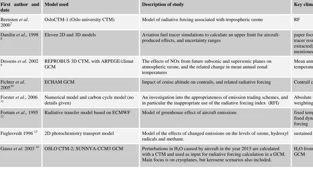
Table 2 Characteristics of included studies

First author and date

Model used Description of study Key climate output(s)

Bernsten et al. 20007

OsloCTM-1 (Oslo university CTM) Model of radiative forcing associated with tropospheric ozone RF

Danilin et al., 1998

8

Eleven 2D and 3D models Aviation fuel tracer simulations to calculate an upper limit for

aircraft-produced effects, and uncertainty ranges

paper focussed on fuel tracer results (not data extracted) but RF also mentioned.

Dessens et al. 2002

9

REPROBUS 3D CTM, with ARPEGE/climat GCM

The effects of NOx from future subsonic and supersonic planes on atmospheric ozone, and the related change in mean annual zonal temperatures

Mean annual zonal temperatures

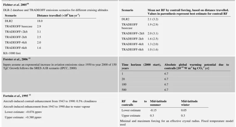
Fichter et al. 200510

ECHAM GCM Impact of cruise altitude on contrails, and related radiative forcing Contrail coverage; RF

Forster et al., 2006

11

Numerical model and carbon cycle model (no details given)

An investigation into the appropriateness of emission trading schemes, and in particular the inappropriate use of the radiative forcing index (RFI)

Absolute GWP; emissions weighting factor

Fortuin et al., 1995

12

Radiative transfer model based on ECMWF Model of greenhouse effect of aircraft emissions fixed temperature forcing;

fixed dynamical heating forcing

Fuglesvedt 1996 13 2D photochemistry transport model Model of the effects of changed emissions on the levels of ozone, hydroxyl

radicals and methane.

sustained GWP

Gauss et al. 2003 14 OSLO CTM-2; SUNNYA-CCM3 GCM Perturbations in H2O caused by aircraft in the year 2015 are calculated

with a CTM and used as input for radiative forcing calculation in a GCM. Main focus is on cryoplanes, but kerosene scenarios also included.

H2O from CTM; RF from

First author and date

Model used Description of study Key climate output(s)

Isaksen et al., 2001

15

OSLO CTM Model of the impact of aircraft emissions on atmospheric ozone and

methane lifetime. Calculated changes in the global distribution of ozone and methane then used to calculate RF of current and future (2015 and 2050) fleets of subsonic aircraft.

RF

Johnson et al., 1996 16

2D CTM Model of transport of trace gases and calculation of their radiative

impact/global warming potential.

GWP; RF

Marquart et al., 2001 17

Calculations of RF, methods vary depending on emission type. Some based on ECHAM climate model.

Model of kerosene vs. hydrogen planes, future scenarios RF, overall and due to:

CO2, O3, CH4, H2O,

contrails, sulphates, soot

Marquart et al., 2003 18

Calculations added to ECHAM GCM Development of a contrail parameterization for the ECHAM GCM contrail cover; RF

Marquart et al., 2005 19

GCM with contrail parameterisation [ECHAM4.L39 (DLR)]

An updated estimate of the radiative forcing of a hypothetical fleet of cryoplanes compared with a conventional aircraft fleet (update of Marquart et al 2001).

RF

Meerkötter et al. 1999 20

Radiative transfer model Parametric study of the instantaneous radiative impact of contrails RF

Minnis et al., 1999

21

Radiative transfer model Model of radiative forcing by persistent linear contrails RF

Morris et al., 2003

22

Trajectory model Model of the effect of aircraft exhaust on water vapour in the lower

stratosphere, and calculations of radiative forcing.

water vapour; RF

Myhre et al., 2001

23

Multistream model Global calculations of radiative forcing due to contrails from aircraft.

Contrail distribution was computed based on aviation fuel consumption and radiative transfer models for solar and thermal infrared radiation.

RF

Penner et al. 1999 1 3D chemical transport models (online & offline)

IPCC intercomparison of models RF, greenhouse gas

First author and date

Model used Description of study Key climate output(s)

concentrations

Pitari et al 2002 24 3D CTM (ULAQ model) Modelling the effect of sulphate particles on RF RF

Ponater et al., 1996

25

ECHAM 3D GCM Model of the global atmospheric response to aircraft water vapour

emissions and contrails

solar radiation; thermal radiation; net radiation

Ponater et al., 1999

26

Atmospheric GCM (ECHAM4) coupled to a mixed layer ocean model (MLO) CTMs used for ozone data - MOGUNTIA used as basis for some of the scenarios

Modelled effect on the climate of ozone changes caused by present and future air traffic.

climate response; surface air temperature; RF

Ponater et al., 2002

27

Novel parameterization of contrails added to ECHAM4

Parameterization of contrails for use in global climate models, and resulting modelled radiative forcing of contrails.

RF

Ponater et al., 2005

28

ECHAM4 GCM with amendments for contrails and with a mixed layer ocean model

Model of climate sensitivity parameter to contrail cirrus climate sensitivity

parameter; mean surface temperature

Ponater et al., 2006

29

ECHAM4 GCM Model of the potential reduction in climate impact by switching from

kerosene to liquid hydrogen fuelled planes

RF; surface temperature

Rind et al., 1995 30 Goddard Institute for Space Studies

climate/middle atmosphere model (GISS/GCMAM).

Modelled experiments of ozone and water vapour perturbations. One scenario includes an aircraft component.

sea surface temperature, air temperature

Rind et al., 1996 31 Goddard Institute for Space Studies (GISS)

global climate middle atmosphere model

Model of the climatic effect of water vapour release surface air temperature

Rind et al., 2000 32 Goddard Institute for Space Studies (GISS)

global climate middle-atmosphere model (GCMAM).

Model of the climatic impact of cirrus cloud increases along aircraft flight paths

surface air temperature; RF

First author and date

Model used Description of study Key climate output(s)

33 _climate

Sausen et al., 2000

34

Combination of linear response models Model of climate response to emissions scenarios CO2 concentration, global

mean sea surface temperatures, sea level changes

Sausen et al., 2005

35

Five CTMs and Climate Chemistry Models: TOMCAT, CTM-2, ECHAM4.L39, LMDz-INCA, ULAQ

New estimates of RF from number of climate models, to update IPCC (1999) estimates for 2000.

RF, with and without cirrus cloud forcing

Stevenson et al., 2004 36

HadAM3-STOCHEM climate-chemistry model.

Model of radiative forcings generated by aircraft NOx emissions through changes in ozone and methane.

RF

Stordal et al., 2005

37

Regression analysis between trends in cirrus cloud and aircraft traffic density; cirrus cloud cover then multiplied by RF of cirrus to get overall RF from aviation. Based on FAST

An investigation of trends in cirrus cloud cover due to aircraft traffic, and calculations of RF from this.

RF

Strauss et al., 1997

38

1D radiative convective model (RCM) Model investigating the impact of contrail-induced cirrus clouds on

regional climate (southern Germany).

solar and ice cloud radiative properties

Valks et al., 1999

39

CTM – RIVM version of MOGUNTIA Model of the effect of present and future NOx emissions from aircraft on

the atmosphere, and the corresponding RF

RF

Williams et al.,

2002 40

Numerical model (no further details) Model of the effect of cruising altitude on the climate change impacts of

aviation. The rationale for restricting cruising altitude is to reduce contrail formation.

% change in fuel burn; altered flight times;

RF estimated, but not really an output of model calculations.

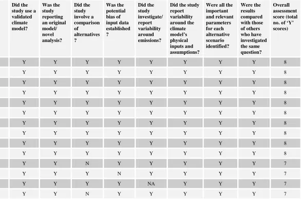
Table 3 Quality assessment of included studies ranked by quality assessment score

Did the

study use a validated climate model? Was the study reporting an original model/ novel analysis? Did the study involve a comparison of alternatives ? Was the potential bias of input data established ? Did the study investigate/ report variability around emissions?

Did the study report variability around the climate model’s physical inputs and assumptions?

Were all the important and relevant parameters for each alternative scenario identified? Were the results compared with those of others who have investigated the same question? Overall assessment score (total no. of ‘Y’ scores)

Fichter et al. 200510 Y Y Y Y Y Y Y Y 8

Gauss et al. 2003 14 Y Y Y Y Y Y Y Y 8

Marquart et al., 2003 18 Y Y Y Y Y Y Y Y 8

Minnis et al., 1999 21 Y Y Y Y Y Y Y Y 8

Penner et al. 1999 1 Y Y Y Y Y Y Y Y 8

Ponater et al., 1996 25 Y Y Y Y Y Y Y Y 8

Ponater et al., 2002 27 Y Y Y Y Y Y Y Y 8

Ponater et al., 2006 29 Y Y Y Y Y Y Y Y 8

Sausen et al., 2000 34 Y Y Y Y Y Y Y Y 8

Strauss et al., 1997 38 Y Y Y Y Y Y Y Y 8

Bernsten et al. 2000 7 Y Y N Y Y Y Y Y 7

Pitari et al 2002 24 Y Y Y N Y Y Y Y 7

Rind et al., 1996 31 Y Y Y Y NA Y Y Y 7

Did the study use a validated climate model? Was the study reporting an original model/ novel analysis? Did the study involve a comparison of alternatives ? Was the potential bias of input data established ? Did the study investigate/ report variability around emissions?

Did the study report variability around the climate model’s physical inputs and assumptions?

Were all the important and relevant parameters for each alternative scenario identified? Were the results compared with those of others who have investigated the same question? Overall assessment score (total no. of ‘Y’ scores)

Dessens et al. 2002 9 Y Y Y ? ? Y Y Y 6

Marquart et al., 2005 19 Y Y Y Y ? ? Y Y 6

Ponater et al., 1999 26 Y Y Y Y ? ? Y Y 6

Ponater et al., 2005 28 Y Y N Y Y Y ? Y 6

Rind et al., 2000 32 Y Y Y Y NA Y ? Y 6

Valks et al., 1999 39 Y Y Y ? N Y Y Y 6

Fuglesvedt 1996 13 Y Y N ? Y Y N Y 5

Morris et al., 2003 22 N Y Y ? N Y Y Y 5

Myhre et al., 2001 23 N Y Y ? N Y Y Y 5

Rind et al., 1995 30 Y Y Y Y N Y ? ? 5

Stevenson et al., 2004 36 Y Y Y Y N ? ? Y 5

Stordal et al., 2005 37 N Y N Y Y ? Y Y 5

Isaksen et al., 2001 15 Y Y Y N N N N Y 4

Marquart et al., 2001 17 Y Y Y N ? ? Y N 4

Did the study use a validated climate model? Was the study reporting an original model/ novel analysis? Did the study involve a comparison of alternatives ? Was the potential bias of input data established ? Did the study investigate/ report variability around emissions?

Did the study report variability around the climate model’s physical inputs and assumptions?

Were all the important and relevant parameters for each alternative scenario identified? Were the results compared with those of others who have investigated the same question? Overall assessment score (total no. of ‘Y’ scores)

Danilin et al., 1998 8 Y Y N N N N N Y 3

Forster et al., 2006 11 N Y Y N N N ? Y 3

Fortuin et al., 1995 12 N Y N N N N ? Y 2

Johnson et al., 1996 16 Y Y N ? N N N N 2

Meerkötter et al. 1999 20 N Y N ? N N ? Y 2

Figure 3. Quality assessment summary

4.2

Assessment of effects of aviation emissions

Results of the included studies are presented in this section. These 35 papers covered a range of original research studies that modelled the effect of aviation on the atmosphere, with outcomes measured in terms of RF, GWP or temperature changes. A range of scenarios was used, in terms of aircraft traffic, model types and parameters. The inputs and major outcomes are summarised in Table 4 - Table 9. The review aims to synthesise the results of these studies in a coherent manner, so that the reader is able to gain an understanding of the current state of the science. This section is sub-divided to separately describe papers presenting results of aviation’s overall effect on RF, GWP and temperature, and that due to carbon dioxide; water, contrails and cirrus clouds; and ozone and aerosols. Where papers are relevant to more than one sub-section they are discussed in turn. While the issue of hydrogen fuelled cryoplanes was not the focus of this review, results from studies which presented data for both cryoplanes and kerosene-fuelled fleets are included, and discussed as a matter of interest for the reader. An overall summary of the results is given in section 3.2.5.

4.2.1 Overall effect of aviation on RF, GWP and temperature

The overall effect of aircraft emissions on the atmosphere, in terms of RF, GWP or temperature variations, is modelled in the five papers reviewed here. The key inputs and outcomes are presented in Table 4.

Penner et al1. This is discussed in more detail, and the context of other similar research, in section 3.2.2. The IPCC Fa1 reference scenario developed by the ICAO Forecasting and Economic Support Group (FESG) using a mid-range growth forecast (3.1% per year) and assuming technology for improved fuel efficiency and NOx reduction, resulted in RF of 0.114 Wm-2 for 2015, and 0.193 Wm-2 for 2050.

In addition to the baseline case, a number of other scenarios were presented by Penner et al1. These included the effect of different air traffic growth rates, introduction of a supersonic fleet of airliners (scenario Fa1H), and focussing on certain emission reduction technologies above others. The lower bound was for scenario Fc1, representing a low-growth rate of 2.2% per year with a subsonic-only airliner fleet, resulting in an RF of 0.129 Wm-2 for 2050. The upper bound was for scenario Edh, representing a high growth rate (4.7% per year) and focussed on low NOx technology, giving an RF of 0.564 Wm

-2

in 2050.

Marquart et al17 focussed on assessing the impact of the introduction of a fleet of hydrogen-powered cryoplanes in 2015, but also reported kerosene fuelled aircraft as a baseline: 0.111 Wm-2 for 2015; 0.132 Wm-2 for 2050; and 0.137 Wm-2 for 2100. In this study, aviation growth was assumed to stop in 2015, accounting for the difference in RF figures for 2050 and 2100 between this study and that by Penner et al1. In a similar study, Ponater et al29 also investigated cryoplanes, and produced a baseline RF prediction for a pure kerosene fleet of 0.128 Wm-2. The predictions for the introduction of cryoplanes in 2015 reduced the RF in 2050 to 0.109-0.115 Wm-2 from Marquart et al17, or 0.0904 to 0.1074 Wm-2 from Ponater et al29.

A surface temperature increase of 0.052K was predicted for 2050 by the IPCC Fa1 reference scenario. Sausen et al34 used a combination of linear response models to assess temperature changes since 1950, predicting an increase of 0.025K in 2050, leading to 0.047K in 2100. Ponater et al29 estimated temperature increase of 0.041K in 2050 for a kerosene aircraft scenario.

The papers reviewed here represent the key studies for global effects of major aviation emissions on the environment using a range of different growth and technology scenarios. The effects of component emissions and their chemistry on the environment are discussed in more detail in sections 3.2.2 to 3.2.4.

4.2.2 Effects of carbon dioxide on RF, GWP and temperature

Papers specifically investigating the effect of carbon dioxide on RF, GWP and temperature are discussed in this section. The key inputs and outcomes are shown in Table 5.

The IPCC paper of Penner et al1 provided a breakdown of the component contributions to its global predictions. Results for 1992 indicated RF of 0.018 Wm-2 due to CO2. Sausen et al

35

scaled the IPCC results to 2000 (0.025 Wm-2) to compare them with their own updated results from the TRADEOFF project of 0.0253 Wm-2. An RF due to CO2 of 0.074 Wm

-2

in 2050 was predicted by Penner et al1 for the mid-range Fa1 scenario. This compares well with the results of Ponater et al29, which predicted 0.0729 Wm-2 in 2050. Marquart

et al

in 2050 due to CO2 of 0.025 Wm -2

(Marquart et el17) and between 0.0196 and 0.020 Wm-2 (Ponater et al29).

Fortuin et al12 investigated the effect of RF due to CO2 from 1943 to 1990, using fixed temperature and fixed dynamical heating assumptions, and reported results for mid-latitude summer and winter. The RF was 0.023 to 0.029 Wm-2 for the mid-latitude summer case and 0.018 to 0.023 Wm-2 for mid-latitude winter. The study also investigated contributions from water vapour, contrails and aerosols, which are discussed in sections 3.2.3 and 3.2.4.

Forster et al11 discussed the use of a radiative forcing index (RFI) as a metric for assessing the impact of non-CO2 emissions on the environment. Emissions from 1950 to 2000 were modelled using an exponential growth model, and emissions were then held constant over a 500 year timescale. The Absolute Global Warming Potential (AGWP) was then calculated for 1, 20, 100 and 500 years, and the effect of CO2 and non-CO2 effects on the AGWP highlighted. From this the RFI was shown to change significantly with time, highlighting the danger in using RFI to account for non-CO2 effects in any assessment of aviation emissions.

The results of Sausen et al34 used the IPCC Fa1 scenario and predicted a temperature increase due to CO2 of 0.024K by 2050, and 0.047K by 2100. This compares well to an increase of 0.026K by 2050 predicted by Ponater et al29.

4.2.3

Effects of

A significant amount of recent research has focussed on the science of water, contrails and cirrus cloud formation from aircraft at altitude. This is a major source of uncertainty in assessing the impact of aircraft emissions on the global environment, as highlighted by Penner et al1. In this section 20 papers are reviewed that present original research, with the key inputs and outcomes of each shown in Table 6 - Table 8.

The effect of water vapour on RF in 2000 was studied by Sausen et al35, and was calculated to be 0.002 Wm-2, which is the same as that reported in the IPCC report by Penner et al1. The radiative transfer model (RTM) study by Fortuin et al12 used simulations up to 1990 and reported RF for mid-latitude regions of between 0.006 and 0.023 Wm-2 in summer, and 0.028 and 0.131Wm-2 in mid winter using a fixed dynamical heating assumption. Ponater et al25 performed a detailed study of the effect of water vapour, using factors of 10, 100, 1000 and 10000, along with sensitivity studies of cloud cover increase by 0.10, 0.05 and 0.02. The study noted that the effect of clouds was much more than that of the water vapour itself, which produced no detectable large-scale climate signal. It was noted that the experiment used was highly artificial and a much stronger enhancement than would ever occur in reality. Rind et al31 performed a parametric study of water vapour effects on RF using a global climate middle atmosphere model. Experiments using water vapour 0.35, 1.5, 35 and 700 times the 1990 aircraft release values showed a measurable effect in the latter two cases only. The cases of 0.35 and 1.5 times 1990 release amounts showed no consistent trend, and the paper therefore concluded that the effect of water vapour does not have a global impact.

and 2100. Ponater et al29 reported RF of 0.0019Wm-2 for kerosene fuelled aircraft in 2050, compared with between 0.0018 and 0.0107Wm-2 for three cryoplane scenarios. Gauss et al14 investigated water vapour effects of cryoplanes for 2015 using a variety of scenarios. Their baseline study for kerosene aircraft resulted in an RF of 0.0026Wm-2, compared with a baseline cryoplane case of 0.0065 Wm-2 and a worst case RF of 0.0625Wm-2 when cryoplane cruising altitude was increased by 3km. The major source of uncertainty was the estimated tropospheric lifetime of aircraft emitted water. The CTM model used here was found to be very sensitive to variations of this parameter. This study only considered water vapour, and not contrail effects.

The overall IPCC assessment of Penner et al1 calculated the RF due to contrails to be 0.100 Wm-2 in 2050, and RF due to water to be 0.004 Wm-2. The level of uncertainty associated with the effect of cirrus clouds caused it to be excluded from the reported results. Sausen et al

35

used a number of climate models in the TRADEOFF project to update the results of Penner et al1 due to contrails, scaled for 2000 (0.039 Wm-2), to 0.010 Wm-2. The effect of cirrus clouds was estimated to be 0.030Wm-2, but with an upper bound of 0.080Wm-2, which was reported in more detail by Stordal et al37. Rind et al32 investigated increases in cirrus cloud coverage along aircraft flight paths using a global climate model. For increases in high-level cloud cover from 0.5% to 5%, RF changed from 0.00 to 2.4 Wm-2. Ponater et al28 used artificially elevated traffic levels (20 x Fa1 inventory) to highlight the effect of cirrus clouds; 3.2% contrail coverage produced an RF of 0.29 Wm-2.

Fichter et al10 calculated the mean net RF due to contrails as part of the TRADEOFF project, and the effect of changing cruise altitude on this for 1992 air traffic data. The baseline case showed an RF, corrected for long wave radiation effects, of 0.0029Wm-2. Increasing cruising altitude by 2000 feet increased RF to 0.0031Wm-2. Reducing altitude reduced RF, with a 6000 feet lower cruising altitude resulting in an RF of 0.0016 Wm-2. Fortuin et al12 used a radiative transfer model to investigate a range of emission effects for 1990. They calculated a local RF due to contrails at mid-latitudes of between -0.15 and 0.30 Wm-2 in summer, and 0.05 and 0.30 Wm-2 in winter.

Future projections of the effect of contrails were included in the cryoplane studies of Marquart et al17 and Ponater et al29. Marquart et al17 predicted kerosene fuelled aircraft to contribute an RF of 0.052 Wm-2 in 2015 and 2050, compared with between 0.0191 and 0.0929 Wm-2 in 2050, calculated by Ponater et al29. These studies highlight the increased effect of contrails due to the introduction of cryoplanes, with Marquart et al17 estimating RF of 0.081Wm-2 in 2015 and 2050, compared with between 0.0156 and 0.0783 Wm-2 for the three different cryoplane scenarios reported by Ponater et al29.

showed that varying the optical depth of the contrails from 0.2 to 0.5 gave an RF of between 0.01 and 0.03 Wm-2 for a 0.1% global mean contrail cover case. A key conclusion of the paper was that the uncertainty of the effect of contrail forcing is a factor of five, due to lack of knowledge of contrail cover and optical depth values.

Myhre et al23 investigated the short wave and long wave contributions to contrail RF using an artificially high 1% contrail cover experiment, and a more realistic 0.09% cover scenario. They highlighted that while short wave radiation provided a negative RF, on balance the net RF was positive, resulting in net RF of 0.12 for both the cloudy and clear condition cases with 1% contrail cover. For the realistic cirrus cloud cover case of 0.09%, the effect of including the diurnal cycle was studied. The net RF dropped from 0.011 Wm-2 to 0.009 Wm-2 when the diurnal cycle was included. Marquart et al18 performed a similar study, showing RF due to contrails rising from 0.0023 Wm-2 in 1992 to 0.0148 Wm-2 in 2050.

Ponater et al27 developed a parameterised model for including contrails within the ECHAM4 GCM, relating the contrail coverage and optical properties to the state of the atmosphere at any given time. It also allowed feedback of the contrails on the net climate effect. This paper was one of the first attempts to include such a detailed contrail model in a GCM.

As discussed in Section 3.2.2, Forster et al11 investigated the use of RFI as a metric for climate change. They calculated an AGWP due to contrails, showing that it remains constant with time due to their short-lived nature and hence non-cumulative effect.

Rind et al32 investigated increases in cirrus cloud coverage along aircraft flight paths using a global climate model. The global temperature response was shown to be linear for increases in high-level cloud cover from 0.5% to 5%, with global surface temperature changing by between 0.1ºC and 2.2ºC respectively. Ponater et al28 used artificially elevated traffic levels (20 x Fa1 inventory) and reported that a 3.2% contrail coverage produced a surface temperature increase of 0.082K.

Strauss et al38 developed a 1D radiative convective model and studied the effect of increased cloud cover over Southern Germany, varying the ice particle size from 2µm to 2000µm. A 10% increase in cloud cover was reported to lead to a surface temperature increase of 1.1 to 1.2K in July, and from 0.8 to 0.9K in October. Their model of current contrail cloud cover over Europe, near 0.5%, results in a surface temperature increase of 0.05K.

4.2.4 Effects of ozone, NOx and aerosols from aviation on RF, GWP and temperature

The direct and indirect effect of aerosols, NOx and ozone on the atmosphere are studied in the 18 papers included in this section. Nitrogen oxides enhance ozone production and reduce methane concentrations. Soot and sulphur dioxide also affect the climate response, both directly and indirectly. The effect of water vapour is discussed in section 3.2.3. The key input and outcomes are presented in Table 9.

The IPCC report of Penner et al1 provides a breakdown of RF due to ozone, methane, sulphate aerosol and soot aerosol for the period 1990 to 2050. The values for the Fa1 scenario for ozone and methane for 2015, from NOx, are 0.040 Wm

-2

ozone of between 0.019 and 0.037 Wm-2 in January and July 2015. Isaksen et al15 predicted RF in 2015 due to ozone to be 0.047 Wm-2 , and that due to methane as -0.032 Wm-2. Ponater et al29 computed a global RF of between 0.0175 and 0.182 Wm-2 for ozone and between -0.0082 and -0.0856 Wm-2 for methane in 2050, indicating the significant level of variability in the simulations. These resulted in a global temperature change of between 0.0114 and 0.0764K due to ozone, and between -0.0046 and -0.039K for methane. Sausen et al34 predicted a temperature change of between 0.010 and 0.097K for 2015 due to ozone using different scaling factors. The study of Rind et al30 showed decreases in stratospheric ozone and increases in tropospheric ozone in 2005. Desssens et al9 also looked at ozone effects using five different scenarios, with mixtures of subsonic and supersonic fleets. For the subsonic only case the ozone decrease was shown to cool the lower stratosphere by -1.6K at 22km over the North Pole. Bernsten et al7 investigated tropospheric ozone and RF from 1900 to 1990, giving a global mean RF of 0.34 Wm-2 in 1990.

Fortuin et al12 performed a global simulation up to 1990 using a radiative transfer model and showed an RF due to NO2 of 0.003 Wm

-2

in summer and -0.001 Wm-2 in winter. The RF due to ozone was between 0.034 and 0.135 Wm-2 in summer and 0.012 to 0.046 Wm-2 in winter, using a fixed temperature model assumption. Sausen et al35 provided an updated estimate for 2000. Compared with IPCC results scaled to 2000, an RF due to ozone was 0.0129 Wm-2, compared with 0.0289 Wm-2 using IPCC data. The methane RF also differed, the new results showed -0.0104 Wm-2 versus -0.0185 Wm-2 from scaled IPCC figures.

Forster et al11 explored the suitability of using RFI as a metric for non-CO2 effects of aviation. Their simulations for 1 to 500 years, with no growth in aviation, showed that the net GWP due to ozone and methane changes from 2.0 to -0.009×10-14 Wm-2kgCO2

-1

yr. Fuglesvedt et al13 showed sustained GWP due to NOx to reduce from 1576 over 20 years, to 148 over 500 years. Johnson et al16 investigated climate sensitivity to a step change of 1 Tg yr-1 in NOx emissions. They reported an increase in RF due to ozone of 0.019594 Wm-2 in 10 years, and an overall step change in GWP of 456.0 after 100 years.

Pitari et al24 investigated the effect of excluding or including sulphur emissions in a climate model, showing a difference of RF due to SO4 from 0.00 to -0.007 Wm

-2

. This induced changes in RF due to ozone from 0.027 to 0.015 Wm-2, although no change in RF due to methane was seen (-0.008 Wm-2 in both cases). The effect of sulphate aerosol on RF was included in the predictions of Penner et al1, giving -0.006 Wm-2 for 2015. This compares well to the results of Marquart et al17 of -0.006 Wm-2 for 2015. The TRADEOFF estimates for sulphate aerosol RF effects in 2000 from Sausen et al35 showed a slight reduction from those of IPCC (Penner et al1 scaled to 2000, from -0.004 to -0.0035 Wm-2. Danilin et al8 performed aviation tracer fuel simulations for 1992 using 11 different global atmosphere models and concluded that the upper limit for RF due to sulphates is -0.013Wm-2. The simulations of Fortuin et al12 from 1943 to 1990 revealed an RF due to sulphate aerosol of between -0.182 and -0.550 Wm-2 for mid-latitude summer, and between -0.141 and -0.421 Wm-2 for mid-latitude winter, using a fixed temperature model assumption.

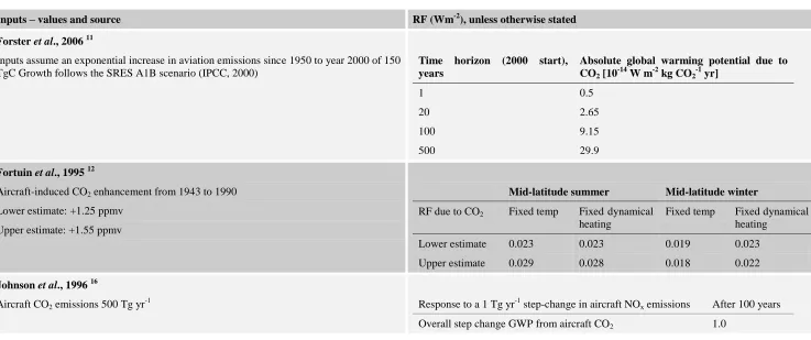
Table 4 Overall effect of aviation on RF, GWP and temperature

Inputs – values and source RF (Wm-2), unless otherwise stated

Marquart et al., 2001 17

Model inputs Kerosene LH2 (cryoplane)

Mass of equal energy 1kg 0.357kg

Emission index H2O 1.26kg (H2O)/kg(ke) 3.21kg ((H2O)/kg(ke)

Emission index NOx 12.6g (NO2)/kg(ke) 1.1 to 5.0g (NO2)/kg(ke)

Global fuel consumption 270.1 Tg(kerosene)

yr-1

96.4 Tg(H2O) yr-1

Global H2O emissions 340.4 Tg(H2O) yr

-1

868.0 Tg(H2O) yr

-1

Global NOx emissions 1.04 Tg(N) yr-1 0.088 to 0.411 Tg(N) yr-1

Emission properties above are for 2015 scenario

2015 2050 2100

Kerosene 0.111 0.132 0.137

Cryo 0.125 to 0.131 0.109 to 0.115 0.098 to 0.104

Morris et al., 2003 22

Emissions for predicted 2015 subsonic fleet in 2015 come from Baughcum et al.

(1988) emissions inventory.41

Emissions for projected fleet of 500 supersonic aircraft come from IPCC.1

Latitude RF Winter RF Summer

Subsonic aviation

54°N standard 0.002 -0.001

54°N extreme 0.008 0.002

82°N standard 0.004 -0.006

82°N extreme 0.012 -0.007

Standard case=monthly mean water vapour perturbation profile

Inputs – values and source RF (Wm-2), unless otherwise stated

Penner et al. 1999 1

Scenario Description

Fa1 Reference scenario developed by ICAO Forecasting and Economic

Support Group (FESG); midrange economic growth from IPCC (1992); technology for both improved fuel efficiency and NOx reduction

Fa2 Fa1 traffic scenario; technology with greater emphasis on NOx

reduction, but slightly smaller fuel efficiency improvement

Fc1 FESG low-growth scenario; technology as for Fa1 scenario

Fe1 FESG high-growth scenario; technology as for Fa1 scenario

Eab Traffic-growth scenario based on IS92a developed by

Environmental Defence Fund (EDF); technology for very low NOx assumed

Edh High traffic-growth EDF scenario; technology for very low NOx

assumed

Total RF 1990 2000 2015 2025 2050

Fa1 0.048 0.071 0.114 0.137 0.193

Fa2 0.048 0.071 0.114 0.136 0.192

Fc1 0.048 0.071 0.114 0.118 0.129

Fe1 0.048 0.071 0.114 0.161 0.280

Eab 0.048 0.068 0.103 0.184 0.385

Edh 0.048 0.083 0.146 0.265 0.564

Global mean surface temp increase (K)

1990 2000 2015 2025 2050

Fa1 0.000 0.004 0.015 0.024 0.052

Fc1 0.000 0.004 0.015 0.023 0.039

Fe1 0.000 0.004 0.015 0.026 0.070

Eab 0.000 0.004 0.014 0.026 0.090

Edh 0.000 0.005 0.019 0.038 0.133

Pitari et al. 2002 24

Scenario 1 includes NOx, H2O and hydrocarbon emissions from aircraft

Scenario 2 includes NOx, H2O, hydrocarbon and sulphur emissions from aircraft

No input values given

Scenario Net RF

1 0.018

Inputs – values and source RF (Wm-2), unless otherwise stated

Ponater et al., 2006 29

Ker – standard, purely kerosene aviation, calculated using IPCC inventories for 1940 to 2050;

cryo1 – technology transition begins in 2015, with EU taking the lead followed by North America in 2020 and S. America, Asia and Middle East in 2025. cryoplanes introduction starts with smallest planes, with long-range aircraft following about 10 years later;

cryo2 – assumes fast transition, starting with gradual world-wide transition of small and medium-sized aircraft in 2015 and of large aircraft in 2025. Scenario results in complete switch to hydrogen fuel by 2050;

cryo3 – starts with world-wide transition later (2020), but proceeds as fast as cryo2 towards the end of the period.

Global RF [W m-2] for 2050

Kerosene (min, max)

Cryo1 Cryo2 Cryo3

Sum of global RF 0.128 (0.1023,

0.1570)

102.2 (83.2, 184.5)

90.4 (74.9,

143.4)

107.4 (87.3, 198.3)

Global temp change (mK) for 2050

kerosene Cryo1 Cryo2 Cryo3

Sum of global temp change 0.0410

(0.0309, 0.0829)

0.0383 (0.0290, 0.0731)

0.0371 (0.0283, 0.0422)

Inputs – values and source RF (Wm-2), unless otherwise stated

Sausen et al., 2000 34 Scenario Description

R Reference case: historical CO2 concentration until 1995, IS92a

thereafter (all natural and anthropogenic sources including aircraft emissions).

Fa1 Standard aircraft emissions scenario: historic data (IEA) until 1995,

NASA for 2015, FESGa (tech option 1) for 2050, 1% annual growth thereafter.

Fa2 As FA1, but for tech option 2

Fe1 Aircraft emissions scenario: historic data (IEA) until 1995, NASA

for 2015, FESGe (tech option 1) for 2050*

Fc1 Aircraft emissions scenario: historic data (IEA) until 1995, NASA

for 2015, FESGc (tech option 1) for 2050*

Eab Aircraft emissions scenario: historic data (IEA) until 1995,

EDFa-base thereafter

Eah Aircraft emissions scenario: historic data (IEA) until 1995,

EDFa-high thereafter

Cτ As Fa1, but aircraft emissions constant for t ≥ τ.

N2015 As Fa1, but no aircraft emissions after 2015

* These two scenarios only run until 2050; others were run until 2100

Temperature change (K)

Year R Fc1 Fa1 Fe1 Eab Eah C1995 C2015 C2050 N2015

1950 0.232 0.000 0.000 0.000 0.000 0.000 0.000 0.000 0.000 0.000

1970 0.305 0.001 0.001 0.001 0.001 0.001 0.001 0.001 0.001 0.001

1990 0.437 0.003 0.003 0.003 0.003 0.003 0.003 0.003 0.003 0.003

1992 0.455 0.004 0.004 0.004 0.004 0.004 0.004 0.004 0.004 0.004

1995 0.483 0.004 0.004 0.004 0.004 0.004 0.004 0.004 0.004 0.004

2000 0.532 0.006 0.006 0.006 0.006 0.006 0.006 0.006 0.006 0.006

2015 0.702 0.010 0.010 0.010 0.010 0.011 0.010 0.010 0.010 0.010

2050 1.230 0.023 0.025 0.028 0.033 0.050 0.018 0.024 0.025 0.015

2100 2.159 0.047 0.086 0.146 0.025 0.036 0.043 0.011

Sausen et al., 2005 35

New estimates of FR from a number of climate models, to update IPCC 1999 estimates for 2000. Scenarios: 1992 data scaled to 2000; IPCC 1999 data scaled to 2000; 2000 (TRADEOFF).

1992

(IPCC, 1999)

2000

(IPCC, scaled to 2000)

2000 TRADEOFF

Total RF (Wm-2)

w/o cirrus

Table 5 Effect of aviation’s CO2 on RF, GWP and temperature

Inputs – values and source RF (Wm-2), unless otherwise stated

Forster et al., 2006 11

Inputs assume an exponential increase in aviation emissions since 1950 to year 2000 of 150 TgC Growth follows the SRES A1B scenario (IPCC, 2000)

Time horizon (2000 start), years

Absolute global warming potential due to CO2 [10-14 W m-2 kg CO2-1 yr]

1 0.5

20 2.65

100 9.15

500 29.9

Fortuin et al., 1995 12

Aircraft-induced CO2 enhancement from 1943 to 1990

Lower estimate: +1.25 ppmv

Upper estimate: +1.55 ppmv

Mid-latitude summer Mid-latitude winter

RF due to CO2 Fixed temp Fixed dynamical

heating

Fixed temp Fixed dynamical

heating

Lower estimate 0.023 0.023 0.019 0.023

Upper estimate 0.029 0.028 0.018 0.022

Johnson et al., 1996 16

Aircraft CO2 emissions 500 Tg yr-1 Response to a 1 Tg yr-1 step-change in aircraft NOx emissions After 100 years