by
WILLIAM JOHN SKIRVING B.Sc.(Hons)
Submitted in fulfilment
of the requirements for the degree of Master of Science
UNNERSITY OF TASMANIA HOBART
any other higher degree or diploma in any tertiary institution, and to the best of my knowledge and belief, this thesis contains no material previously published or written by another person, accept when due reference is made in the text of the thesis.
a leisurely sail. However, his efforts were thwarted by a very smelly
obstacle ... mud! Even if he could have forded the mud between himself and his
yacht, he still had to contend with the fact that there was no water under the yacht
on which to sail! What could he do? Naturally, he went and told his local member
of parliament about his predicament, and so began the Government's concern over
TABLE OF CONTENTS
PAGE
ABSTRACT iii
ACKNOWLEDGEMENTS iv
LIST OF FIGURES vi
LIST OF PLATES
x
LIST OF TABLES xi
LIST OF SYMBOLS AND UNITS xii
CHAPTER 1:
CHAPTER 2:
CHAPTER 3:
CHAPTER 4:
INTRODUCTION 1
A. Sediment Transport 1
B. Measurements of Suspended Sediment Loads 5
C. Aims 14
METHODOLOGY 18
A. Measuring Suspended Sediment Concentrations 18 B. Estimating Suspended Sediment Transport 29 C. Sediment Transport Characteristics
D. Techniques Applied in this Study a. Hand Samples
b. Turbidity Measurements
THE STUDY AREA A. Geology and Soils B. Climate
C. Vegetation and Land Use
ESTIMATES OF SUSPENDED SEDIMENT TRANSPORT
A. Sediment Transport at Ballroom B. Sediment Transport at Corra Linn
CHAPTER 5:
CHAPTER 6:
CHAPTER 7:
BIBLIOGRAPHY APPENDICES:
SEDIMENT PROVENANCE A. Soil Erosion
B. Factors Affecting Suspended Sediment Concentration
93
94100 C. Case Studies of Sediment Provenance 103 a. A Case Study of Three Flood Events 103
b. A Logging Episode 115
DISCUSSION
CONCLUSION
1. Filtration Method
2. Underestimates of Suspended Sediment
119
128
132 150
Transportation 153
3. Turbidity Meter Electronics - A Description 15 5 4. Estimates of Sediment Transport - Effects
ABSTRACT
This thesis investigated the suspended sediment transportation of the North Esk River, Tasmania. The investigation was divided into two sections, the origins and the quantity of sediment transported. With respect to the origins, it was found that the main contributors to the suspended sediment load were recently denuded areas, i.e. recently logged areas and ploughed farmland. For example, 7 6 lt of sediment was estimated to have come from a 50ha logging coupe in only 320hours.
A single beam turbidity meter, based on light attenuation, was designed and constructed to monitor the sediment concentrations of the river. The results from.this turbidity meter were used in conjunction with discharge data to derive a sediment rating curve. This curve was applied to daily discharge records to derive long term estimates of sediment transport.
ACKNOWLEDGEMENTS
I am indebted to my supervisors,
Mi
Albert Goede and Dr Manuel Nunez, for their continued support and time given without reservation during the development and conduct of this study. Their guidance in the drafting of this thesis is also appreciated.I would like to thank the Water Research Laboratory for providing the funding for the first year of this project.
I am in debt to Paul Waller and Kelvin Michael for their ever-ready assistance throughout the course of the study. Without their help, parts of this study would not have been possible.
I am eternally grateful to my parents for their continued support.
During the field work for this study, I was rarely without company for support and safety. Three people stand out in this respect, Lauren and Alexandria Steele, and my mother; thanks for the many hours you spent in the field with me, this project would not have been as thorough without you. Other people who deserve a vote of thanks for helping in the field are: Julie Shepherd, David Gibson, John Cover, David and Kim Hood, Merrie Michael, Steve Levis, Alison Jones, Fiona Melling, Sally Shepherd, Gary and Ellen Hennessy, and anyone who I may have missed.
Thanks to Douglas Steane and the Rivers and Water Supply Commission for their help with discharge data. Thanks also to Andrew Livingstone and the Hydrology section at the H.E.C.
For their assistance during the project, thanks to the staff of the Central Science Laboratory and the Geography Department at the University of Tasmania. Also, thanks to the Geography Department at James Cook University for their advice and support during the writing of this thesis.
Thanks also to Dr Bruce Brown, Mark Mabin, Lance Bode and Eddy Rowe for their assistance.
LIST OF FIGURES FIGURE 1: FIGURE2: FIGURE3: FIGURE4: FIGURE5: FIGURE6: FIGURE7:
FIGURE SA:
FIGURE SB:
FIGURE9:
FIGURE 10:
FIGURE 11:
FIGURE 12:
FIGURE 13:
FIGURE 14:
PAGE
The Tamar River drainage basin.
U.S. single stage suspended-sediment sampler.
Delft Bottle; schematic diagram showing flow pattern.
2
20
22
Schematic diagram of a nephelometer. 25
Schematic diagram of a transmissometer. 27
Cross sections of suspended sediment concentration for the North Esk River at Ballroom. 36
The North Esk River drainage basin. 3 7
Cross sections of suspended sediment concentration from various points within the North Esk River basin.
Cross sections of suspended sediment concentration 39
from various points within the North Esk basin. 40
Circuit diagram of the turbidity meters electronics. 43
Turbidity meter section. 44
Turbidity meter mounting. 48
Turbidity meter calibration. 50
Relief of the North Esk River basin. 52
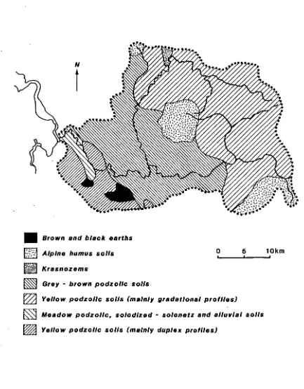
FIGURE 15: Soils of the North Esk River basin. 54
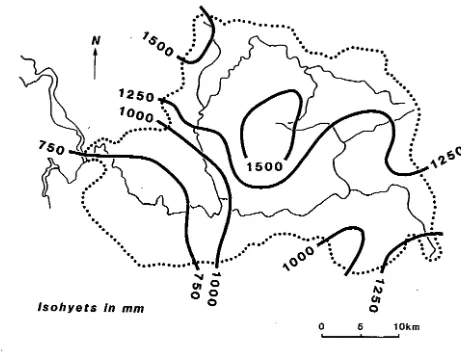
FIGURE 16: Average annual rainfall for the North Esk River
basin. 58
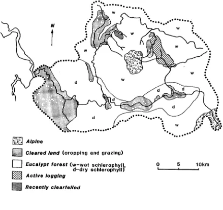
FIGURE 17: Vegetation and landuse within the North Esk River
basin. 61
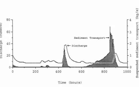
FIGURE 18: Discharge and suspended sediment transport data for the North Esk River at Ballroom (5pm, 7th September, 1986 to 9pm, l 7th October, 1986). 70
FIGURE 19: Discharge and suspended sediment transport for the North Esk River at Ballroom (The first 540 points of
Figure 18). 71
FIGURE20: Suspended sediment transport vs discharge for the North EskRiver at Ballroom (7th to 30th September,
1986). 72
FIGURE21: Log-log plot of suspended sediment transport vs discharge for the North Esk River at Ballroom (7th
to 30th September, 1986). 73
FIGURE22: Suspended sediment transport vs the rising stage of discharge for the North Esk River at Ballroom ( 7th
to 30th September, 1986). 75
FIGURE23: Sediment rating curve for the North Esk River at
Ballroom. 76
FIGURE24: Daily average discharge for the North Esk River at
Ballroom during 1967. 80
FIGURE25: Total suspended sediment transport estimates of
FIGURE26: FIGURE27: FIGURE28: FIGURE29: FIGURE30: FIGURE 31: FIGURE32: FIGURE33: FIGURE34: FIGURE35: FIGURE36:
Total suspended sediment transport estimates of the North Esk River at Ballroom for 196 7.
Histogram of estimates of annual suspended sediment transport for the NOrth Esk River at Ballroom.
Stage-discharge rating curve for the North Esk River at Corra Linn.
Suspended sediment rating curve for the North Esk River at Corra Linn.
LoWl.og plot of daily average discharge for the North 82
85
86
87
Esk River at Corra Linn against the discharge at Ballroom for 1961-63 and 17 days during 1985-86. 90
Histogram of estimates of annual suspended sediment transport for the North Esk River at Corra Linn.
Areas affected by gully erosion within the North Esk River basin.
Areas affected by rill erosion within the North Esk River basin.
92
96
97
Areas affected by mass movement within the North Esk
River basin. 101
Vegetation and landuse, including the water sampling sites, within the North Esk River basin. 104
North Esk River hydrographs from Ballroom for floods
FIGURE37: Predicted and measured suspended sediment transport rates for the North Esk River at Ballroom (lst to l 7th
LIST OF PLATES PLATE 1: PLATE2: PLATE3: PLATE4: PLATES: PLATE6: PLATE 7: PLATE8: PLATE9:
PLATE 10:
PLATE 11:
PLATE 12:
PLATE 13:
PLATE 14:
PLATE 15:
PAGE
Campbell CR21 Micrologger with cassette tape for
data storage. 45
Prototype turbidity meter, mounted in a small stream. 49
Eucalypt forest, upper North Esk River. 60
Grazing Pasture with eucalypt forest in the background,
North Esk River at Ballroom. 60
Active logging, upper St Patricks River. 62
Cropping on the river flats (barley) with grazing in the foreground, North Esk River at Ballroom. 64
Ploughing on the river flats, lower St Patricks River. 64
The North Esk River at Corra Linn Gorge. 66
Hydrographic recorder, North Esk River at Ballroom. 67
Hydrographic recording site for the North Esk River at Ballroom.
Bank erosion, North Esk River downstream from the Ford River junction.
Logging coupe in the upper North Esk River.
Electronic drying oven with desiccators.
Electronic scale and Whatman GF/C Microfibre Filterpaper.
Millipore suction filtration equipment.
LIST OF TABLES
TABLE 1:
TABLE2:
TABLE3:
TABLE4:
TABLES:
TABLE6:
Selected river suspended sediment yield data from Strakhov (1967), Holman (1968) and Milliman and Meade (1983) for several continents.
PAGE
7
Summary of some published data on soil erosion losses from agricultural and forested plots and catchments in eastern Australia. Compiled by Olive and Walker
{1982) and the author. 11
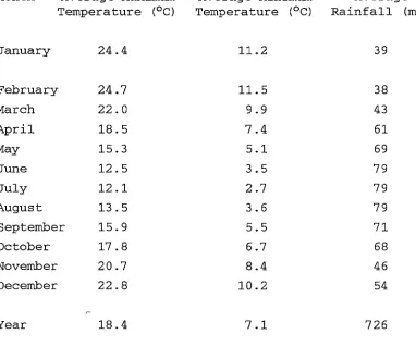
Launceston climatological data; Averages over the
period 1908 to 1987
55
Average monthly rainfall data for eight stations within the North Esk River catchment area. 57
Peak suspended sediment concentration for 22 .sites within the North Esk River basin during three separate floods.
Rainfall for floods A, B and C.
105
LIST OF SYMBOLS AND UNITS
SYMBOLS
*
shear velocity uWO fall velocity of a particle
d particle size
D depth of flow
c
sediment concentrationt'o ratio of grain shear stress
toe critical shear stress
La sediment transport
Q
dischargeT total sampling time dt sampling interval
0 scattering angle
PVC polyvinyl chloride LDR light dependent resistor
UNITS
nm nanometre
µm micrometre
mm millimetre
m metre
km kilometre ha hectare
t tonne
v volt
pF picofarad
.a
ohmkO. kilo-ohm mg milligram
g gram
1 litre
min. minute
s second
oc
degree CelsiusCHAPTER 1: INTRODUCTION
In June 1984, Unisearch Ltd and the Water Research Laboratory of the University of New South Wales, were commissioned to undertake a two year investigation into the causes of siltation within the Tamar River, in particular its upper reaches near Launceston. The study was directed by Professor D. N. Foster and was supervised by the Tamar River Improvement Committee, established by the Government of Tasmania to examine and report on problems related to the development and beautification of the Tamar River.
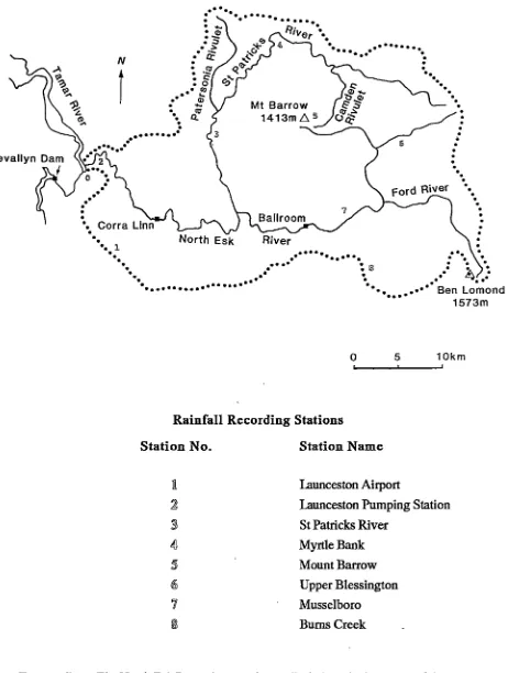
As part of this study, the University o~ Tasmania was contracted by the Water Research Laboratory to investigate the quantities and origins of suspended sediment entering the Tamar River from its tributaries. Consequently, a project was set up to investigate the suspended sediment load of the North Esk River (Figure 1), considered to be representative of the whole Tamar Basin. The main aim of this project was to estimate the annual suspended sediment load of the North Esk River, with a view to extrapolating the findings to the entire Tamar catchment. A lesser aim of the project was to investigate suspended sediment provenance within the North Esk Basin.
The Tamar River is a large estuary located in North Eastern Tasmania (Figure 1). It extends for 69.5 km from Bass Strait at Low Head to Launceston where it terminates at the confluence of the North and South Esk Rivers. Tidal effects extend one kilometre up the South Esk River and two kilometres up the North Esk River. Its drainage basin is one of the largest in the state, approximately
11,000 km2• Eighty-seven percent of the Tamar catchment is drained by only two of its tributaries; the North Esk River which has a catchment area of 1067 km21 and the South Esk River which has a catchment area of 24,680 km2.
0
0 I
Figure 1:
50 km I
••• Tamar River catchment boundary
1 St Patrich River
2 North Esk River
3 South Esk River 4 Macquarie River
5 Llffey River
6 Meander River
7 Tamar River
8 Great Lake
period sea level rose by approximately 60 m to about its present level, resulting in the flooding of the Tamar River and the formation of the drowned river valley which is now the Tamar Estuary. Since the sea level reached its present level, the estuary has been gradually filled in with sediments brought down by its tributaries, particularly the North and South Esk Rivers which drain approximately one seventh of the total area of Tasmania. This infilling has been largely restricted to the upper half of the estuary. The lower reaches still retain many of the characteristics of a drowned valley. (Foster, et al., 1986)
The Tamar River has three distinct periods of usage. The first period was between 1804 and 1890, when the river retained much of its natural state. Water depths were sufficient to meet the needs for the type and size of ships using the river. During this period, port works were primarily concerned with navigational aids and tugs to assist the movement of ships. (Foster, et al., 1986)
The second period (1890 to 1965) was a period in which continuous and increased dredging was needed to meet the requirements of larger and larger ships using the Port of Launceston. This dredging increased the channel depth in the upper reaches of the estuary by redistributing the silt from the upper to the lower half. Also during this period, the advent of steam powered vessels meant that the need for tugs was disappearing. (Foster, et al., 1986)
The third period began in 1965 and has continued to the present. At the beginning of this period, the major port facilities were shifted down river to meet the requirements for larger ships. As a result of this shift, the need for dredging was reduced. (Foster, et al., 1986)
from two sources. The tidal flow is bringing sediment from the lower half of the estuary, and the tributaries are providing 'new' sediment from the upstream catchment." This thesis provides information about the tributaries' contribution to the suspended sediment within the Tamar Estuary.
A. SEDIMENT TRANSPORT
Whether or not a river has the competence to move the materials that it encounters depends on its speed and turbulence (Cooke and Doomkamp, 1974). A river may carry material as bed load, saltation load, suspended load, or as solution load. Bed load is composed of material too large to be carried upwards in turbulent eddies, but in times of high discharge it may be moved along the river bed by sliding, rolling or saltation. Saltation load is the part of the bed load which may in periods of very high-energy conditions in the river, be bounced along the channel floor. The material is never able to stay in suspension for long.
Some authors prefer to include the saltation load within the bed load (Einstein et al., 1940; Chorley, 1969; Hall, 1984; and Rodda, 1985), since the saltating particles from time to time supplement the bed load. Suspended load is carried in the body of the current. The degree of coarseness of suspended particles varies with velocity, and especially with the degree of turbulence. (Chorley, 1969 and Vanoni, 1975)
Solution loads and bed loads were not considered in this study. From the outset it was assumed that, in causing siltation of the Tamar River, solution loads would have a minor effect in comparison with suspended sediment (Rivers and Water Supply Commission, 1983). Also, this variable was already being monitored by the Water Research Laboratory.
The bed loads do not reach the Tamar River, since there is at least one dam or weir on each of the lower reaches of the main tributaries, which prevents movement ofbed load. There are no records to indicate pre-weir (pre 1950s) bed load transport rates, however visual observations made by'the author show little or no build-up of bed material behind these weirs, hence it may be assumed that bed load transported by the tributaries, to the Tamar River, prior to the construction of the weir, was negligible. If the bed loads remain in the system, they would be continually broken down, by chemical and physical processes, into particles which are small enough to be eventually flushed out as suspended sediments. (Foster et al., 1986)
B. MEASUREMENTS OF SUSPENDED SEDIMENT LOADS
ecosystems. Recently concern has grown over the concentration and absorption of radionuclides, pesticides, herbicides and many organic materials by sediments; data on sediment movement and particle characteristics are needed to determine the extent and cause of this potential danger to health. (Gower, 1980; Walling and Webb, 198lb; Rodda, 1985; and Pigram, 1986)
Table 1 is a comparison of average annual suspended sediment transport rates of rivers in each of the continents (except Antarctica), taken from three separate studies, Strakhov (1967), Holman (1968) and Milliman and Meade (1983). Each study exhibits similar trends, with Australia and Africa having the lowest average sediment yield, and Asia the largest. On a global scale, Holman (1968) demonstrated that approximately 19x109 t of sediment reach the ocean per year, a quantity equivalent to a denudation rate of 75 mm per 1,000 years. However, Milliman and Meade (1983) suggest a global figure of 13.5x10⁹ t of sediment per year reaches the ocean.
World data of sediment loads of rivers show that generally, the denudation rates of catchments range between 1and10,000 tlkm2/year. However, if the data are restricted to catchments less than 10,000 km2 with an annual rainfall between 1,200 and 1,500 mm (i.e. similar rainfall to the North Esk basin, see Chapter 3) the world average denudation rate is 600 tlkm2/year. (Walling and Kleo, 1979)
"Disturbance of surface soil for agriculture, mining and urbanization is a major contributor towards increased sediment loads in rivers world-wide ... " (Loughran, 1984). How the activities of man affect the natural amounts and distribution of erosion and sediment transport must be determined if future changes in land use are to be carried out in such a way as to minimize increases in erosion rates. Accelerated erosion of fertile soil due to mismanagement is common, and changes in the sediment pattern resulting from man's activities can have far-reaching social and economic repercussions (Pigram, 1986).
CONTINENT AREA SEDIMENT YIELD (km2x106) ( t/km2 /year)
Strakov Holman Milliman & Meade
Europe 9.7 43 35 50
Asia 44.9 166 600 380
Africa 29.8 47 27 35
North &
Central 20.4 73 96 84
America South
America 18.0 93 63 97
Australia 8.0 32 45 28
erosion control practices, by the construction of structures in the river and by channel modification schemes. (Detwyler, 1971; Gower, 1980; Rodda, 1985; and Stott, et al., 1986) However, quantifying the effects of man's activities on suspended sediment load in rivers is difficult. Finlayson and Wong (1982) found that relationships obtained in small catchment studies cannot be easily extrapolated to other areas. Regardless of this, most suspended sediment studies are still conducted on small catchments, due to their manageability, e.g. Imeson and Vis (1984).
Sheet and rill erosion are much reduced by increasing the density of vegetation, as demonstrated by Wischmeier and Smith (1965) who found a 250% decrease in soil loss after planting a high quality grass cover on fallow land. Conversely the removal of forest can greatly increase erosion. Brown and Krygier (1971), O'Loughlin (1974), O'Loughlin et. al. (1978), Nolan and Janda (1981) and Cassells et al. (1982) all report an increase in sediment yield following deforestation. Management practices during logging can also greatly affect suspended sediment loads in rivers, Megahan (1972), Pearce and Griffiths (1980), Burgess et al. (1981), Reid et. al. (1981), and Megahan et. al. (1986). In the Eden area, N.S.W., the impact of clear-fell logging in a dry sclerophyll catchment has been examined by Rieger, et al. (1979) and Burgess et al. (1981). Increases of up to 150% in sediment loads following the construction of roads and the start of logging were reported. The suspended sediment loads apparently returned to close to pre-logging levels after twelve months. Most of the increase in sediment load was explained by poorly sited and constructed roads, and sediment loads tended to decrease as logging continued. _
levels in approximately twelve months. A further episode of increased sediment transport accompanied the logging, with a trend towards pre-logging loads after two years. Langford et al. (1982) whilst working in the same catchment, found that after logging of the Blue Jacket Creek there was no return to pre-logging suspended sediment concentrations. The difference between these findings and those of Kriek and O'Shaughnessy (1975) was interpreted as being due to differences in road drainage, with Blue Jacket Creek having longer and steeper sections of road draining towards the stream.
While studying 11 small drainage basins in the Keuper region of central Luxembourg, Imeson and Vis (1984) found that at any given specific discharge, the maximum suspended sediment concentration for cultivated catchments was at least twice that from the forested catchments.
Ketcheson et. al. (1973) identify two ways in which agricultural practices can effect the generation of stream sediment; (1) erosion of soil from the land surface, and (2) erosion of soil from streambank areas. Agriculture may contribute passively to the processes affecting stage 2. In stage 1, agriculture is instrumental in determining the kind of soil cover available to protect the soil surface. This protection may be vegetative as determined by the crops and cropping practices used, or non-vegetative as determined by tillage practices and surface roughness. For instance, direction of ploughing is important, as on short low-angle slopes, contour ploughing produces some 50% less sediment than ploughing uphill and downhill (Piest and Spomer, 1968). In stage 2, agriculture may be instrumental in providing more or less vegetation cover, and controlling the extent of farm animal activity on the banks of streams passing through agricultural land.
agricultural activities to river sedimentation. While studying suspended sediment movement patterns of Midwestern streams, U.S.A., Wilkin and Hebel (1982) found that cropped floodplains are the most severely eroded lands in the watershed, followed by cropped lands bordering the floodplains. They concluded that the majority of cropped uplands may not be nearly as important in determining suspended sediment levels in streams as is generally thought.
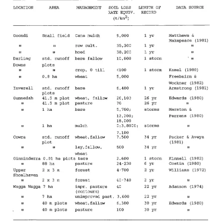
Table 2 is a summary of published data on soil erosion losses from hill slope plots and small catchments in eastern Australia, compiled by Olive and Walker (1982). It contains 24 examples, two from forested plots, and the rest from agricultural land (e.g. bare, fallow, pasture and cropped areas). In general, Table 2 suggests that soil losses per unit area from small plots are greater than from large plots, and these are greater than the few values available from small catchments. This undoubtedly reflects the fact that the larger the system studied, the greater the opportunities of redeposition of eroded material within it (Finlayson and Wong, 1982).
The maximum reported soil losses (38,200
tlkm
2) occurred from deeply rilled cane fields in northern Queensland during one year of observation (Matthews and Makepeace, 1981), see Table 2. Even under cane mulch, erosion losses were 9,000tlkm
2• A single storm event experienced in the Darling Downs, southern Queensland (Kamel, 1980), removed soil at the rate of 10,000tlkm
2• These values are far in excess of the soil loss tolerance levels of 500-1,200tlkm.2/yearwhich have been developed for conservative management of agricultural
soils in the U.S. (Olive and Walker, 1982). Adamson (1974) and Edwards (1980),
'
.whilst studying erosion rates of pasture, found that the bulk of soil erosion losses over a long period could be attributed to a few storm events.
LOCATION AREA MANAGEMENT SOIL LOSS LENGTH OF DATA SOURCE RATE EQUIV. RECORD
(t/km2 )
Goon di Small field Cane mulch 9,000 1 yr Matthews &
Makepeace (1981)
II II row cult. 35,300 1 yr II
II II hoed 38,200 1 yr II
Darling std. runoff bare fallow 10,000 1 storm II
Downs plots
II II crop, 0 till <100 1 storm Kamel (1980)
II 0.8 ha wheat 5,000 Freebairn &
Wockner (1982)
Inverell std. runoff bare 6,400 1 yr Armstrong (1981)
plots
Gunned ah 41.5 m plot wheat, fallow 20,100 26 yr Edwards (1980)
II 41.5 m plot pasture 70 26 yr II
II 1 ha bare 5,700; storms Marston &
12,200; Perrens (1980)
18,000
II 1 ha mulch 0;3,8000; storms II
7,100
Cowra std. runoff wheat, fallow 7,500 34 yr Packer & Aveya
plot (1981)
II II ley,fallow, 800 34 yr II
wheat
Ginninderra 0.01 ha plots bare 2,600 1 storm Kinnell (1982)
II 88 ha pasture 24-230 6 yr Costin (1980)
Upper 2 x 3 m forest 4-700 2 yr Williams (1972)
Shoalhaven
II 2 x 3 m forest 40-740 2 yr II
Wagga Wagga 7 ha impr. pasture 40 22 yr Adamson (1974)
(contours)
II 7 ha unimproved past. 3,600 22 yr II
II 40 m plots wheat, fallow 6,300 30 yr Edwards (1980)
II 40 m plots pasture 100 30 yr II
[image:27.567.49.472.141.586.2]Reservoir construction can create many problems as demonstrated by the silting of the San-Men reservoir on the Yellow River (Hathout, 1979). McManus and Duck (1985) found similar problems with the Glenfarg and Glenquey reservoirs in Scotland. Paskett (1982) suggests that proper land
I
management techniques would decrease reservoir sediment accumulation. Problems can also occur downstream of a dam. Pemberton (1981) found that clearing of the reservoir area before closure of the Stateline dam, on the Smith's Fork River, U.S.A., exposed sediments that were flushed through the dam and deposited in the gravel spawning reach of the river for a distance of about 9 km
downstream from the dam. Urban development is the most dramatic change of land use and the accompanying construction can greatly increase sediment yield. Walling and Gregory (1970) demonstrated that the annual sediment yield of some 200 V'J.an2 from a small agricultural catchment was increased by a factor of four after urbanization. Wolman (1967) compared sediment yields from four landuse types. He found that undisturbed forests provided the least sediment to rivers, with urban areas, grazing land and cropped land all having progressively larger sediment yields. Wolman suggests that, of the four Ianduse types, urban land provides the least sediment after forested land. He points out that during urban construction, these areas can provide up to 1 OOO times more sediment to the river systems than any other Ianduse type. Since Wohµan's work, other studies have shown similar results (Williams, 1976; Warner, 1976; Lam, 1978; Gower, 1980; and Lootens and Lumbu, 1986).
From the above discussion it can be seen that human activities can have a profound effect on the quantity of sediment transported by rivers. The magnitude of these effects vary, although they tend to be greatest when the landuse decreases the amount (or changes the type) of vegetation cover. However, these effects are not always permanent, since a number of studies have shown that after logging, the initially high sediment loads of rivers have returned to low loads of pre-logging after a period of one to two years (Kriek and O'Shaughnessy, 1975; Rieger et al., 1979; and Burgess etal., 1981).
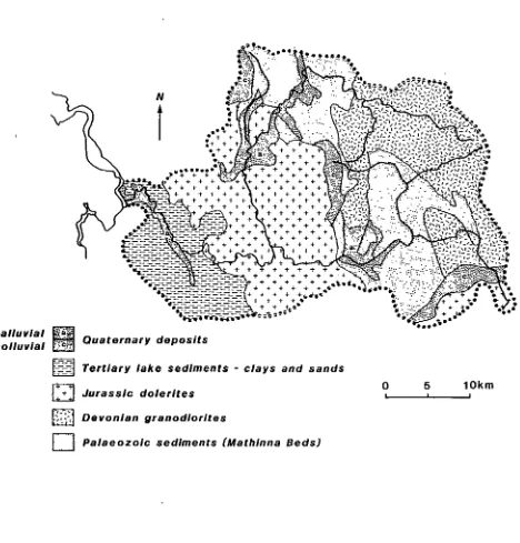
Man's activities in the North Esk Basin can be categorized into five groqps, forestry, farming, recreation, urbanization and road building. Forestry activities include selective logging, clear felling and replanting, all of which necessitate road building and changes to the natural vegetation. There are two main farming activities, cropping and grazing. Cropping is mostly confined to the river flats, whilst grazing also occurs on hills which surround the river flats. Almost all grazing in the area is carried out on improved pastures, therefore both fanning types involve ploughing, and often include irrigating. There are a wide range of recreational activities within the North Esk Basin. They include bushwalking, camping, caravaning, fishing, rafting, canoeing, many types of sports and snow skiing. Of these, skiing is possibly the most disruptive, since it requires the grooming of ski slopes. The population within the North Esk Basin is very scattered, with only a few very small towns. Therefore urbanization is only a small part of man's activities within the area. Lastly, all the above activities require an extensive transport network within the area, if they are to function properly. As a result of this, road building plays a major role in man's activities within the North EskBasin.
changes have persisted, is not certain. Other studies also indicate that the relationship between man's activities and suspended sediment origins is complex. Consequently, this study will not attempt to directly attribute suspended sediment origins to individual landuses, rather it will investigate the existence of preferred geographical locations for suspended sediment origins.
C. AIMS
Due to the limited resources available, a detailed study was restricted to the suspended sediment load of the North Esk River Basin (Figure 1). The North Esk River was not only small and manageable, but was also considered to be representative of the Tamar River tributaries. The North Esk basin has at least one example of every type of landuse found in the Tamar catchment, as well as most rock types.
Only one previous study of suspended sediment loads has been carried out in Tasmania. Olive (1973) sampled three small catchments in southeastem Tasmania, Mountain River, Browns River and the Snug River. He measured both suspension and solution loads over a one year period. The measurements were -, used to estimate denudation rates for the period. The applicability of Olive's study to the present study is very limited, since the streams he measured are considerably smaller.
Meteorological differences between the two study areas are also evident. North Eastern Tasmania receives most of its rain from orographic processes, whilst frontal systems dominate the rainfall in South Eastern Tasmania. The average annual rainfall for each of the study areas also differ. Mountain River, Browns River and the Snug River have average annual rainfalls of 900, 7 50 and 700 mm respectively, which are smaller than the North Esk River's average annual rainfall of 1,160 mm.
The aims of this investigation are somewhat different to those of Olive's study. The first and main aim was to derive an estimate of the mean annual suspended sediment transport of the North Esk River, and the second was to investigate the geographical origins of suspended sediment within its catchment.
The study will use suspended sediment rating curves to calculate suspended sediment transport rates. However, as explained earlier, man's activities in the area have almost certainly changed the suspended sediment loads within the river system. This means that there is a high likelihood that the relationship between suspended sediment load and river discharge has also changed. Consequently, this study will restrict itself to current estimates of suspended sediment transport and will therefore not be directly concerned with historic transport rates.
Data sources from the North Esk River catchment are very limited. There are no usable records of suspended sediment concentrations available for the North Esk River. Therefore a large number of measurements were made so as to provide the suspended sediment concentration values needed for the study. To facilitate these measurements, a large amount of time was invested in the design, construction and installation of a turbidity meter, which was used to measure concentrations of suspended sediment at hourly intervals under a wide range of discharges. The data from the turbidity meter were supplemented with hand samples from the study area.
discharge of the North Esk River, which will be used in conjunction with the suspended sediment rating curve (derived <luting the study) to estimate the current mean annual suspended sediment transport.
The thesis firstly discusses the various ways by which rivers transport sediment, and then presents results of some previous sediment transport studies. The first part of Chapter 2 examines suspended sediment sampling techniques: including a literature review of the various ways of estimating suspended sediment concentrations and transport in rivers; and a description of the sampling techniques used in this study, including a detailed description of the turbidity meter's design and application. The last part of Chapter 2 describes the suspended sediment transport characteristics of the North Esk River, e.g. the cross-sectional profile of the suspended sediment concentrations. The study area is described in Chapter 3. This description includes the geology, soils, climate, vegetation and landuse within the North Esk River basin.
Estimates of annual suspended sediment transport rates for the North Esk River are presented in Chapter 4. These estimates are made for the North Esk River at two locations, Corra Linn (near its mouth) and Ballroom (about halfway up the river). The estimates are then extended to provide estimates for the South Esk River and the whole Tamar River basin. In this chapter an averaging technique (the RUME technique), which provides improved estimates of the annual sediment transport rates, is presented.
CHAPTER 2: METHODOLOGY
A. MEASURING SUSPENDED SEDIMENT CONCENTRATIONS
There are many techniques available to measure suspended sediment concentration in rivers (Stichling, 1968; Task Committee on Sedimentation, 1969; McCave, 1979; Graf, 1971; Loughran, 1971; Shaw, 1983; and Ward, 1984). These techniques can be placed in one of two categories; direct methods {water sampling and sediment traps), and indirect methods {radiation attenuation).
The simplest method for the determination of suspended sediment concentration is to take a known volume of water, filter it and determine the weight of material retained on the filter. In the initial stages of the development of samplers, an open container or bucket was used to dip samples from a river. However, this method was shown to cause significant errors (Ward, 1984). This instrument was followed by the ~ottle or closed container type, which could be opened and closed instantaneously at any selected depth. Later, instantaneous samplers of the horizontal trap type, which orientated themselves in the direction of flow, were developed. (Task Committee on Sedimentation, 1969 and Vanoni, 1975)
bottle and connected to the end stoppers. To set the bottle, these are pulled out and connected to a release mechanism. There are many minor variants of these types of samplers, and they are relatively easy to constru~t (e.g. Duursma, 1967).
The single stage sampler has been developed as an aid in obtaining information on flashy streams, particularly those in remote areas where observer services are not available. It is used to obtain a sample at a specific depth and on the rising stage only (Loughran, 1971). Two versions of this type of sampler are shown in Figure 2. The sampler operates on the siphon principle and therefore the velocity in the intake is not equal to the stream velocity. The vertical intake nozzle shown in Figure 2(a) eliminates plugging from surface debris but does not take a sample of acceptable accuracy when sand particles are present. In contrast, the horizontal intake nozzle shown in Figure 2(b) increases the accuracy with respect to the sand particles in the flow but also increases the danger of plugging due to surface or near surface debris. (Loughran, 1971; Vanoni, 1975; Ryan, 1981; and Ward, 1984)
With careful operation, the single stage sampler can be used to obtain supplementary information on sediment concentration at selected points in the vertical profile. Because of the limitations of the sampler, concentration data so obtained must be used with caution in the determination of the mean concentration inanystream. (Ward, 1984)
Sample container
Air exhaust
...__
Intake
(A) Vertical intake (B) Horizontal
intake
The requirements of an ideal integrating suspended sediment sampler have been summarized by Nelson and Benedict {1951) and are as follows: (i) The velocity at the entrance of the intake tube should be equal to the local stream velocity; (ii) the intake should be pointed into the approaching flow and should extend upstream from the zone of disturbance caused by the presence of the sampler; and {iii) the sample container should be removable and suitable for transportation to the laboratory without loss or spoilage of the contents. Furthermore, the sampler should: (iv) Fill smoothly without sudden inrush or gulping; (v) permit sampling close to the streambed; (vi) be streamlined and of sufficient weight to avoid excessive downstream drift; (vii) be rugged and simply constructed to minimize the need for repairs in the field; and (viii) be as inexpensive as possible, while consistent with good design and performance. Integrating hand samplers have been used by Zakaria (1979), Allen and Petersen (1981), Ryan (1981), Singhal et al. (1981) and Lootens and Lumbu (1986).
Pumping samplers have been used in suspended sediment studies since 1968. (Task Committee on Sedimentation, 1969) They are designed so that they can automatically obtain a continuous record of sediment concentration by sampling at a fixed point at specific time intervals. The velocity in the intake is not equal to the stream velocity, and the intake does not always meet the requirements of an ideal sampler since it often does not point into the flow. However, the pumping sampler can be rated or calibrated by comparing mean concentrations determined with it to mean values in the river cross section determined from samples collected with standard depth or point integrating sampling equipment. (Vanoni, 1975 and Ward, 1984) Many studies have used pumping samplers, e.g. Walling and Teed (1971), Ryan (1981), Finlayson and Wong (1982) and Lam (1984).
LONGITUDINAL SECTION
CROSS-SECTION
0
Flow into picture®
Flow out of pictureFigure 3: Delft Bottle; schematic diagram showing flow pattern.
volume of the bottle, drops its load of suspended sediment in the bottle and passes out through the holes in the rear. It catches material >50 µm in diameter. In order to determine concentration, a measurement of flow speed at the nozzle height of the
bottl~ is also required. (McCave, 1979)
There are many indirect methods for measuring suspended sediment concentrations (Austin, 1973; Gibbs, 1974; Jerlov and Nielson, 1974; McCave, 1979; Shaw, 1983; and Ward, 1984). The two most commonly used methods involve the monitoring of density and optical properties. Density monitoring uses the nuclear direct sensing technique, and has been used in studies to monitor suspended sediment load in rivers as early as 1970 (McHenry et al., 1970; Welch and Allen, 1973). More recently, the technique has been used by Berke and Rakoczi (1981), Tazioli (1981) and Xianglin et al. (1981). In this method, gamma rays are passed through the turbid water and their attenuation is measured. This attenuation allows for the calculation of the density of the medium through which the rays pass. A simple comparison between the density of the turbid water and the density of clean water will enable the sediment load to be determined. In a discussion on sediment and dissolved loads of major world rivers, Knighton (1984) suggests that, a range of between 7% and 91 % of the total sediment load is carried in solution. When using density monitoring to measure the suspended sediment load of a river, it is often necessary to independently measure the solution load, so that it may be subtracted from the water density method, leaving the suspended sediment value. For this reason, conductivity measurements are often taken in conjunction with the density technique.
sensor, whereas in the latter the sensor measures the light scattered (reflected and refracted) by suspended particles. The measuring instruments are the beam transmission meter or transmissometer, the scatterometer or nephelometer, and the secchi disc. Both transmission and scatter are functions not only of the number, but also the size, refractive index and shape of the particles. Thus different suspensions of the same concentration will have different optical properties. It is therefore undesirable to calibrate optical sensors in terms of artificial turbidity standards when studies are carried out in a natural environment (Austin, 1973).
Figure 4 is a schematic diagram of a nephelometer. The principle behind a nephelometer is relatively simple. Scattered light from a collimated beam of light, passing through a column of water, is collected by a photocell which has been positioned at an angle 0 from the light beam. The angle 0 is the scattering angle.
Turbidity is then related to the amount of scattering. Tikhonov and Goronovskii ( 1984) described a single beam nephelometer which was designed to automatically monitor water quality.
When monitoring suspended sediment concentrations, nephelometers have the apparent advantage that only suspended particles cause significant light scattering (Austin, 1973), so that coloured but sediment-free water will not yield spurious results. However, such water does attenuate the light beam. At high concentrations of suspended sediments the beam can be depleted to near zero, resulting in erroneous results (Dunkerley, 1984). For these reasons, light scatter is generally used in conjunction with light attenuation (e.g. Briggs, 1962; Fleming,
1967; Vanous, 1981; Dunkerley, 1984; andGilvearandPetts, 1985).
'
''
' Scattering'
''
' :volume.
~---·---~~---""\M@tfl\ Light
source
.
--- ---
-\~~\)~---'
'
'
'
'
'
'
'
'
'
'
'
'
'
'
'
Light
' '
Photocell\:>
Figure 4: Schematic diagram of a nephelometer. 0 is the scattering angle. Scattered
can only be done by taking simultaneous water samples for gravimetric analysis. With a rough calibration curve, the disc depth does provide a quick estimate of conditions and this is its chief value.
The transmissometer is based on the principle of light absorption. Parallel light suffers a decrease in intensity on passing through turbid water because of absorption and scattering by water and particles. Absorption by particles is highly. correlated with wave length, and organic particles exhibit strong absorption in the blue (at approx. 450 nm) with another peak in the red region of the spectrum (at approx. 670 nm) (McCave, 1979).
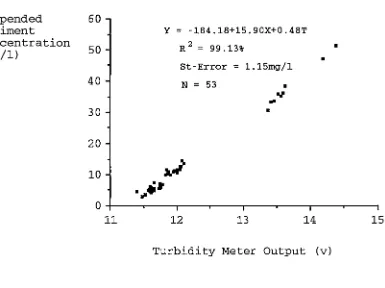
Figure 5 is a schematic diagram of a transmissometer. A known intensity of light flux is aimed, over a fixed path length, through turbid water and onto a photocell. The resultant intensity of light is measured and compared to the initial light intensity to determine the light attenuation. This is then related to turbidity. Single beam transmissometers were successfully used by Brabben (1981) to monitor sediment loss from drainage basins supplying water to two reservoirs in East Java.
There are various types of transmissometers available on the market. Some are placed in the turbid water when in use, others remain out of the water, and have the water pumped past the sensing unit. A double-beam device is described, with a summary of the principle, by Thom (1975), Grobler and Weaver (1981) and Ward (1984). The double-beam system eliminates the problem of fouling of the lens assuming that both lenses are equally contaminated. Buiz (1970) compared two turbidity meters, the Sigrist photometer (a nephelometer) and the Askania turbidimeter (a transmissometer). This study provided no conclusive evidence that one was better than the other. Dunkerley (1984) described a low-power infrared turbidity meter which used a combination of nephelometric and transmission measurements to arrive at a turbidity value.
Light source
~
o
-
---~o-..
__.,.
Fo
.I
I.
P'LL
Figure 5: Schematic diagram of a transmissometer. The incident light flux F 0 is scattered and absorbed so a smaller flux F L is received at the end of the light path L.
although this method has many drawbacks, (Burz, 1970; Austin, 1973), it has often been used successfully to monitor suspended sediment concentration (Walling, 1977a; Brabben, 1981; Grobler and Weaver, 1981; Lammerts van Bueren, 1984; and Finlayson, 1985).
All of the above techniques for measuring suspended sediment concentration in rivers require calibration by direct sampling methods. Unfortunately, while the sampling methods are reasonably well standardized, the laboratory procedures for separating the sediment from the water appear to be of variable efficiency and reliability (Loughran, 1971).
The filtration technique is by far the most common method of separating particles from water samples (Dyer, 1979). Loughran (1971) has described a number of techniques based on filtration. They are rather similar, but have two significant differences. The first difference is in the technique itself. While all techniques require filtering the water sample (often with vacuum filtration apparatus) through a filterpaper, one group requires desiccating by drying the filter paper and residue (usually in an oven) and then weighing them. The weight of the filter paper is subtracted to obtain the weight of the sediment. The second group requires burning the filter paper and sediment after filtration, and the residue is weighed. A constant value for the remaining paper ash is often subtracted to obtain the weight of the sediment, although there are ashfree filter papers on the market, e.g. Whatman. (Loughran, 1971)
The second difference is in the type of filter paper used. At present, there is no international standard filter paper for use in the filtration of suspended sediment (Foster, pers. comm.). Loughran (1971) described four laboratory techniques associated with four different studies, each using a different filter paper.
The laboratory techniques used in this study are described in Appendix 1. To preserve consistency, the author followed the techniques used by the Water
B. ESTIMATING SUSPENDED SEDIMENT TRANSPORT
The simplest method for determining the instantaneous suspended sediment transport of a river is by using one of the direct methods. This is comparatively easy, since sediment particles move at essentially the same velocity as the flow. When measurements of sediment concentration are combined with measurements of water discharge, the transport rate of the sediment is derived. To obtain an unbiased measurement of sediment concentration, either depth integrating samplers are used or a knowledge of the cross-sectional characteristics of sediment concentration is needed. The main drawback of this technique is that it is time consuming as well as providing only an instantaneous, rather than a representative value.
There are two fundamental ways to estimate the suspended sediment transport of rivers. They are theoretical methods and empirical methods.
Many attempts have been made to relate sediment transport rates to the flow conditions in rivers, since it is relatively easy to obtain measurements of the flow parameters. A great deal has been acco~plished, in this regard, in developing theories of suspended sediment transportation through consideration of the mechanics of turbulent flow of liquids. Some of the more notable examples of these theoretical models are Einstein (1950), Laursen (1958), Blench (1966), Ackers and White (1980), Celik (1982) and van Rijn (1984).
Celik (1982) presented a method for predicting the suspended sediment concentration of a river, which was based on the k-E turbulence model, used by Nakagawa et al. (1975) and Ueda et al. (1976). Celik's method was one of the first attempts to use the velocity and eddy-viscosity distributions with a second order turbulence-closure model in calculating suspended sediment concentration distributions.
various types of sediment material. Calculations are made using the k-e turbulence model and relating the mass transfer coefficient to the turbulent eddy viscosity distribution which is also calculated as a part of the solution.
Van Rijn (1984) uses a different approach. His method computes the suspended sediment load through the depth-integration of the product of the local concentration and flow velocity. The method is based on the computation of the reference sediment concentration from his bed-load transport model. The method is calibrated with measurements of concentration profiles. A verification analysis, using about 800 suspended sediment measurements, demonstrates that about 7 6% of the predicted sediment concentrations are within 0.5 and 2 times of the measured values.
Empirical methods involve the estimation of sediment transport from continuous discharge data using relatively infrequent sampling of sediment concentrations. Two standard ways of doing this are to multiply mean concentration by mean discharge (the averaging technique), and to use a rating curve to predict unmeasured concentrations.
The averaging method, as described by Walling and Webb (198la), involves the estimator:
T/At
La = I, CjQj At j=l
where La = sediment transport C = concentration Q = discharge
T = total sampling time
At = sampling interval for each sample
By far the most popular empirical method for estimating the suspended sediment transport of a river is the sediment rating curve. The sediment rating curve has two basic forms, the concentration I river discharge curve and the suspended sediment transport/ river discharge curve. The former curve is derived by correlating simultaneous instantaneous measurements of suspended sediment concentration and river discharge. The latter curve correlates the product of suspended sediment concentration and river discharge (rate of suspended sediment transport) with river discharge. Both forms are power curves (Dunne and Leopold, 1978; Knighton, 1984; Ferguson, 1985), and enable the prediction of suspended sediment transportation from the record of river discharge. This technique involves average discharge values which are applied to a sediment rating curve to determine the corresponding transportation rate. Since the form of the rating curve is a power function, which is usually derived from instantaneous values, the use of average discharge values will provide underestimates of the true transportation rates (see Appendix 2). The size of these errors are generally in proportion to the temporal size of the average used. For instance, Walling (1977a) suggests that yearly totals of sediment transport calculated with the use of hourly discharge averages underestimate the true value by approximately 10 percent, whereas a similar calculation with the use of daily discharge averages can underestimate the true value by as much as 50 percent.
This problem has been known since 1956 when Colby stated that " .... an instantaneous sediment rating curve is theoretically not applicable to the direct computation of daily sediment discharges from daily water discharges .... ". Despite this warning, many researchers still insist on applying daily discharge data to rating curves which have been derived from instantaneous samples (e.g. Hall, 1967; Imeson, 1969; Nilsson, 1971; Temple and Sundborg, 1972; Douglas, 1973; and Al-Ansari etaJ 1977).
produce underestimates (explained above) and secondly, the conversion of sediment concentration to transport negates the validity of the regression as both variables are a function of discharge. (Olive and Rieger, 1984)
To overcome the second problem some authors have based the regression model on sediment concentration rather than instantaneous load, (Loughran 1976 and 1977; Geary, 1981; Walling and Webb, 1981a; and Lootens and Lumbu,
1986). This technique also has two main problems. The first problem is the same averaging problem as the other technique (described above). The second problem was described by Loughran (1976) as:" ... the wide scatter of points on sediment concentration vs discharge plots can make this an inferior technique for the calculation of transport rates ... ",however, he goes on to say that regardless of this problem, this is still a useful technique.
Although it may be argued that sediment transport (sed. cone. x disch.) vs discharge regressions produce spurious correlations, since discharge is a part of both variables (Kenney, 1982), sediment transport is a real variable (regardless of how the data are derived), and consequently the relationship is still valid. Some authors continue to use 'sediment transport vs discharge' rating curves rather than
(
'concentration vs discharge' rating curves, even though the improvement in correlation is spurious (Nolan and Janda, 1981; Mimikou, 1982; Akrasi and Ayibotele, 1984; Makhoalibe, 1984; and Foster et al., 1986).
Leitch (1982) calculated loads using the flow duration series rather than the discharge records. Further refinements of the regression model involved the separation of rising and falling stage data and the determination of two rating curves (Loughran, 1976 and 1977; Walling, 1978; and Geary, 1981).
the occurrence of high sediment concentrations and that in most years the sediment concentrations greatly exceed those computed by rating curves." Kellerhals et al (1974) came to similar conclusions. They found that rating curves for the Red Deer River Basin, Alberta, Canada, significantly underestimated the occurrence of peak sediment concentrations.
Campbell (1977) calculated that yearly total suspended sediment transport maybe underestimated by as much as 40%. Geary (1981) and Olive et al. (1980), working on separate rivers in Australia, found that the sediment rating curve underestimated the actual sediment transport rate by 72% and 83% respectively. Olive et al. found that there was little improvement in the prediction using hourly (instead of daily) flows.
"Obviously serious difficulties are apparent in the sediment rating curve model." (Olive and Rieger, 1984) The major sources of error are related to the basis of a single simple relationship between sediment and discharge. Olive and Rieger (1984, 1985 and 1986) have recognized hysteresis effects in the relationship, by looking at sediment vs discharge through time.
Ferguson (1987) compared the two common empirical methods of estimating suspended sediment transport in rivers (described above). He found that both the averaging method (described by Walling and Webb, 1981a), and the sediment rating curve technique, underestimate the actual sediment transport.
C. SEDIMENT TRANSPORT CHARACTERISTICS
In alluvial streams, the concentration of coarse material transported in suspension depends mainly upon velocity, concentration of fine sediment, bed configuration, and the shape of the measuring section (Graf, 1971; Bogardi, 1974; Vanoni, 1975; Garde and Ranga Raju, 1978; Celik, 1983; and Van Rijn, 1984). Therefore, the concentration of the coarse material in suspension may increase or decrease from section to section, even though the water and total sediment discharge remain uniform.
The suspended sediment concentration generally is at a minimum at the water surface, and at a maximum near the stream bed. The coarsest fractions of the suspended sediment, which are usually sand, exhibit the greatest variation in concentration from the stream bed to the water surface. The fine fractions, i.e., the silt and clay, are usually uniformly distributed over the depth of the stream, or nearly so (Vanoni, 1975; Celik, 1983; and Van.Rijn, 1984).
Momentary or instantaneous fluctuations in suspended sediment concentrations are related to scale and intensity of stream turbulence and particle size of sediment in the bed of the stream. Maximum deviations from mean concentration values are to be found in streams where the suspended sediment consists largely of sand. In contrast, minimum deviations from mean concentration values occur in streams where the suspended sediment consists largely of silt and clay. Thus, the amount of the momentary fluctuation in concentration of the suspended sediment at any depth varies with the ratio of the concentration of the sand fraction to the total concentration. The amount of fluctuation also is affected by the bed configuration. (Celik, 1983)
The lateral distribution of suspended sediment at a stream cross section varies with velocity and depth, channel slope and alignment, bed form, particle size of sediment in transport, and inflow from immediate upstream tributaries (Vanoni, 1975; Garde and Ranga Raju 1978; Celik, 1983; and Van Rijn, 1984).
and concentration usually increases from the inside to the outside of the bend. Secondary circulation undoubtedly plays an important part in lateral distribution for both straight and curved channels, but at present little is known of this phenomenon (Vanoni, 1975).
Before a regular sampling program could be devised for this study, it was necessary to determine the nature of the cross-sectional profile of suspended sediment concentration at various points within the North Esk River system. For this reason, thirteen cross-sectional profiles were measured. All measurements were taken by hand with a Van Dom type sampler (see 'Section D' in this chapter for a description of the hand sampling technique used in this study).
Twelve cross-sections were measured whilst wading and one from a flying fox. The wading samples were taken upstream of the wader, so that the wader did not affect the flow and hence the sample. Also care was taken not to include the saltation load in the samples. The samples were taken at 1/5, 1/2 and 4/5 of the river depth. If the depth was not sufficient for three independent vertical samples then either two samples, taken at 1/5 and 4/5 of the river depth, or one sample, taken at 1/2 of the river depth, were taken. Each cross-section took an average of approximately half an hour to complete.
Eight cross-sections were measured at the junction of two rivers. These were all taken upstream of the junction. The sites for these cross-sections were carefully chosen so that they were far enough upstream not to be influenced by back-water effects from the junction.
Discharge = 2.5 cumecs
4.1 4.0 3.8 4.3 3.8 4.1
4.8 3.5 4.7 4.2 3.8 3.9
5.8 3.5 3.9 3.8 3.9
14/8/86
Discharge 3.1 cumecs
3.3 2.6 3.3 2.5 3.0
3.3 2.4 2.3 2.4 2.8 2.6
3.4 2.9 3.0 5.5 3.2
9/9/86
Discharge = 10.0 cumecs
5.9 4.6 4.8 4.3 4.7
6.1 5.0 5.4 5.4 5.9
5.7 4.2 5.3 6.0 4.8
20/9/86
Discharge = 11. 5 cumecs
11. 9 11. 7 12.0 10.0 11.2
10.7 11.5 11.4 11.2 10.7
10.5 11.2 10.2 11.0 11.5
*26/9/86
Discharge= 29.3 cumecs
Ave Current = 0.3 m/s Mean = 4.1 mg/l · St.dev.= 0.6 mg/l
Gauge Board = 0.80 m Ave Current = 0.3 m/s
Mean = 3.0 mg/l St.dev.= 0.7 mg/l
Gauge Board = 1.16 m Ave Current = 0.9 m/s
Mean = 5.2 mg/l St.dev.= 0.6 mg/l
Gauge Board = 1.22 m Ave Current = 1. 0 m/s
Mean = 11. 0 mg/l St.dev.= 0.6 mg/l
Gauge Board = 1.69 m Ave Current = 2.7 m/s
48.4 48.2 46.9 47.0 48.0 48.4 47.1 Mean = 47.7 mg/l'
St.dev.= 0.7 mg/l
0.5
Scale
(metres)
*
samples taken from flying-fox, due to fast current1.0
l
O-t-~-r~--.~~..-~~
Figure 6:
0 1 2 3
Cross sections of suspended sediment concentration for the North Esk River at Ballroom. All measurements in milligrams per litre. Samples taken at V5, V2, and 4/5 of the river height.
.
•.··
···
... .
. .
...
Ri11er·· •••
41 ••••
.. ..
• •••••••••·
.
.
•• 1
.
•
.
•
.
•. . .
•.
• •
.
.
• •.
.
·.
..
.
..
. .
... .. ..
:
.
..
·. .
••
.
.
••• •• : Im.
.
• • ~ •.
•• •••• • •• • q • ••
•• • • • •• • • • • • •• • •• • • • • •.
....
• •• • Ben Lamond 1573m0 5 10km
Rainfall Recording Stations
Station No. Station Name
Il Launceston Airport
2 Launceston Pumping Station
31 St Patricks River
~ Myrtle Bank
~ Mount Barrow
(6) Upper Blessington
fl Musselboro
[image:53.565.56.518.62.674.2]i&S Bums Creek
measured on the 6/8/86 has a value of 5.8 mg/I in the bottom left of the cross section, which is 1. 7 mg/I greater than the mean for that cross section. Also, the cross section measured on the 14/8/86 has an anomaly situated in the centre close to the bottom. This concentration of 5.5 mg/I is 2.5 mW! larger than the mean for this cross section. Both of these anomalies occur in samples which were taken close to the river bed. They may contain some sediment from the saltation load as well as suspended load. Since there are only two samples of this type, it may be assumed that the saltation load is not significant during low flows at these cross sections (Figure 6). However, it is unrealistic to assume that the saltation load is going to remain inactive at higher flows, when the currents are much stronger. Due to the sampling techniques applied in this study (i.e. single point measurements rather than depth integrating samples), only suspended sediment has been monitored. The saltation load, along with the bed load, has not been monitored. This is a realistic approach, since the study is directed towards estimating the contribution of the North Esk to the accumulation of sediment in the Tamar estuary. Weirs on the lower reaches of the North and South Esk Rivers prevent the saltation load and the bed load from reaching the estuary, as explained previously (Chapter I).
The data in Figure 6 are only representative of the cross sectional profiles of suspended sediment concentrations for velocities of less than 2. 7 m/s. Chorley (1969) and Celik (1983) maintain that at velocities of~l m/s the transport of sand is approximately uniform through all parts of the cross section. Hence, for the purposes of this study, it will be assumed that the cross sectional profile of suspended sediment concentration within the North Esk River at Ballroom is consistently homogeneous.
It can be seen from Figure 8A and 8B that homogeneous cross sectional
St Patricks River (at the North Esk Junction)
12/11/85 Discharge= 2.05 cumecs Current = 0.11 m/s
1.2 1.1 1.6 1.1 0.7 1.5 1.4 0.9
1.8 2.0 1.4 1.7 1.4 1.2 1.3 1.3
Mean = 1 . 3 mg I 1
St.dev.= 0.4 mg/l
7/12/85 Discharge= 7.09 cumecs Current = 0.30 m/s
7.5 7.5
Me an = 7 . 9 mg I 1
St.dev.= 0.7 mg/l
0.5
Scale
(metres)
1.0
l
O+---.--~---~
0 1 2 3
North Esk River (at the St Patricks Junction) 13/11/85
7/12/85
Discharge= 3.30 cumecs
Discharge
5.0 3.8 4.0 3.7 4.2 4.4
10.8 cumecs
12.0 11.2 10.0
Current = 0.50 m/s
Mean = 4 . 1 mg I 1
St.dev.= 0.4 mg/l
Current·= 1.51 m/s
Mean
=·
11. ~ mg/lSt.dev.= 0.9 mg/l
Figure SA: Cross sections of suspended sediment concentration from various points within the North Esk basin. All measurements in milligrams per litre. Samples taken at 115, 1/2, and 4/5 of the river height.
St Patricks River (at the Camden Rivulet Junction) 29/11/85 Discharge= 2.21 cumecs Current = 0.50 m/s
\ 1.1 1.9 1.2 1.2 1.1 2.2
J
Mean = 1.5 mg/lSt.dev.= 0.5 mg/l
Camden Rivulet (at the St Patricks River Junction)' 29/11/85 Discharge= 0.54 cumecs Current = 0.63 m/s
\.. 6.4 6.3 6.6 ) Mean = 6.43 mg/l
St.dev.= 0.15 mg/l
North Esk River (at the Ford River Junction) 30/11/85 Discharge = 1.95 cumecs
l
l8.4 19.1 19.0 19.0 18.718.6 17.7 18.4 )18.9 18.8 19.1 19.0
-Current= 0.59 m/s
Mean 18.8 mg/l
St.dev.= 0.2 mg/l
Ford River (at the North Esk River Junction)
30/11/85 Discharge = 1.37 cumecs Current = 0.40 m/s
l
5.4 5.8 6.0 6.0 6.1 5.8 5.8 ~.8 ). 5.6 5.9 5.6 5.7 5.9 5.7 ~
0.5
Scale
(metres)
1. 0]
0 -+---r----.---.---.
0 1 2 3 4
Mean = 5.8 mg/l St.dev.= 0.2 mg/l