Systematic Luby Transform Codes and their Soft Decoding

SYSTEMATIC LUBY TRANSFORM CODES AND THEIR SOFT DECODING

T. D. Nguyen, L. L. Yang and

L. Hanzo

School of ECS, University of Southampton, SO17 1BJ, UK.

Tel: +44-23-8059 3125, Fax: +44-23-8059 4508

Email:

[email protected], http://www-mobile.ecs.soton.ac.uk

Abstract– Luby Transform codes (LT) were originally designed for the Binary Erasure Channel (BEC) encoun-tered owing to randomly dropped packets in the statistical multiplexing aided classic wireline-based Internet, where transmitted packets are not affected by the fading or noise of the propagation environment of the wireless Internet. For the sake of transmitting data over the BEC routinely encountered in statistical multiplexing aided wireless In-ternet - style scenarios, we applied the belief propagation algorithm for decoding LT codes and designed a novel ver-sion of LT codes, which we refer to as systematic LT codes. When using soft decoding of the proposed systematic LT code, the decoding process becomes capable of prevent-ing the potentially avalanche-like inter-packet error prop-agation. For example, the systematic LT(1000,3000) code achieved aBERbelow10−5_atE

b/N0 = 3.5dBafter six decoding iterations. An even lowerEb/N0 of2.7dB was required, when using a longer systematic LT(10000,30000) code for transmission over the AWGN channel. In the combined BEC-AWGN channel theBERrecorded at the output of the systematic LT(1000,3000) code was about

10−5atEb/N0= 4.5dB, when encounter an erasure prob-ability ofPe= 0.1.

1. INTRODUCTION

LT codes [1] were originally designed for the Binary Era-sure Channel (BEC) channel, where transport packets may be erased with an erasure probability ofPe. When applying

LT codes for transmitting data over wireless channels con-taminated by Rayleigh fading and inter-symbol interference (ISI), the packets may become contaminated, which may re-sult in catastrophic inter-packet error propagation during LT decoding [2]. LT codes were originally designed for error-free BEC channels. For the sake of using LT codes to pro-tect data for transmission over the wireless Internet, where fading, noise and packet erasures are encountered, numerous researchers endeavoured to improve the achievable perfor-mance [2] [3] [4]. Naturally, the complexity of these schemes

The financial support of the EPSRC, UK and that of the EU is gratefully acknowledged

tends to be increased. For the sake of improving the error cor-rection capability of LT codes, in this paper we propose the soft decoding of LT codesusing the probabilistic decoding technique of Low Density Parity Check Codes (LDPC) [5]. The outline of the paper is as follows. Section 2 analyses the disadvantages of the LT codes, when applying the mes-sage passing algorithm and detail the design ofsystematic LT codes. Section 3 analysessystematic LT codesusing extrin-sic information transfer (EXIT) charts and Section 4 charac-terizes their performance over the wireless Internet channels. Finally, Section 5 provides our conclusions.

2. LT CODE DESIGN FOR SOFT DECODING AND THE SYSTEMATIC-LT CODE

LT codes were originally designed for hard-decoding [1] in the context of the BEC. The error propagation phenomenon of the LT decoding process is portrayed in Fig 1. For the sake of avoiding this detrimental effect, they have been combined with various forward error correcting (FEC) codes [2] [4]. These combined schemes substantially mitigated the effects of error propagation. However, the attainable performance improvement of these schemes were still limited owing to the employment of hard-decision aided LT decoding. For the sake of circumventing this deficiency, we introduce the novel concept of soft LT decoding based on the classic belief-propagation technique applying Tanner Graphs. We com-mence our discourse by introducing the concept of single-bit packets. The LT codes having larger packets will be consid-ered as generalized the scenario. The soft LT decoding pro-cess is based on the classic concept of LDPC decoding. Given the generator matrixGof the LT code, we calculate the Par-ity Check Matrix (PCM)H of the LT code similarly to that of a classic LDPC code, namely by dividing the LT code’s generator matrix into two matrices, where AandB have a size of (K×K) and (K×M), respectively. We choose the non-singular matrixAbased on the conventional LT decoding process. Then the PCM is calculated as

S2 S3

S2 S3

S2 S3

S2 S3

S2 S3

S2 S3

S1

S1 1

S1

S1

S1

Source packets

LT−encoded packets

An error part of

1 P2 P3 P4

st

LT decoding cycle

2

1

3

LT decoding cycle

nd

LT decoding cycle

4

LT decoding cycle

5

LT decoding cycle

The last LT decoding cycle

S P

P2

P2 P3

P3

P4

P4

P3

P4

P4

P3

LT−encoded packets

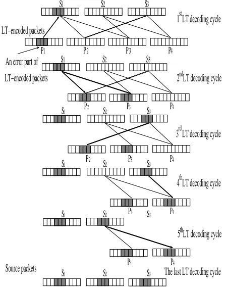
Fig. 1. An example of error propagation in the LT hard-decoding process, when the LT decoder receives packets af-fected by the channel error

To elaborate a little further, the filled circles and the filled

Fig. 2. A tree-based representation of LT code

squares of Fig. 2 represent the LT check nodes and the LT check nodes, respectively, while the horizontal lines connected to the variable nodes represent the intrinsic information pro-vided by the channel’s output. Let us assume that the circular node at the top of Fig. 2 represents thekthvariable node in the block ofN number of single-bit LT encoded packets, which is also termed as the root node [6]. The root node receives information from the check nodes it is connected to at the level seen below it in Fig. 2 and those check nodes also re-ceive information from the variable nodes they are connected to at the next level down, etc. The dotted lines in Fig. 2

indi-cate that the above process is repeated further by expanding the tree. The number of connections associated with a vari-able node of the LT code - excluding the line representing the intrinsic information - indicates the column weight of this particular message node, while the number of connections as-sociated with an LT check node represents the corresponding row weight. The column weight and row weight of the LT PCM are related to the degree distribution of LT packets. The LT decoding process is implemented in the same way as the classic LDPC decoding procedure. Initially, the LT coder’s soft values are set to a value corresponding to the de-modulator’s soft output. The decoder’s soft values ofRa

i,jand

Qa_i,jwhich denote the LLRs passed from the check nodes to the variable nodes and vice versa are then iteratively updated after each decoding iteration as follows:

tanh(Ri,j 2 ) =

Y

n∈{Ci},n6=i

tanh(Qn,j

2 ), (2)

where we have

tanh(x/2) = e x₋₁

ex_{+ 1}. (3)

After each iteration, the LT decoder outputs its tentative hard-decision and checks, whether the product of the correspond-ing codeword and the transpose of the PCMHis equal to zero i.e whether a legitimate codeword was produced. If not, the LT decoding process will be continued in an iterative fashion, until the output codeword becomes legitimate or the maxi-mum affordable number of iterations is exhausted. For the sake of improving the performance of LT codes at highEb/N0 values, we invoke hard-decoding after the last LT decoding cycle in order to erase the low-confidence LT packets, namely those, which have low Logarithm Likelihood Ratios (LLRs). We employ a low complexity packet-reliability evaluation tech-nique based on the average LLR of the packet.. However, the soft LT decoding process based on the LT code’s PCM ex-hibits some deficiencies owing to the following two reasons:

• the LT code’s PCM contains many zero-columns, which degrades the performance of the LT code, when using the above mentioned soft decoding process.

• The conventional non-systematic LT code will impose error propagation, when using the above-mentioned hard-decoding process for the sake of recovering the original information packets from the erroneously decoded LT-encoded packets, as seen in Fig.1.

1 0 1 0 0 0 1 1 0 0 1 0 0 0 1 1 1 0 0 0 0 0 1 1 0 1 0 0 1 1 1 1 0 1 0 0 0 1 1 1 1 1 0 0 0 1 1 1 0 1 0 1 0 1 1 1 0 1 0 0 0 0 1 1 0 1 0 0 0 0 0 0 0 1 0 0 0 0 1 0 0 0 0 0 1 1 1 1 0 1 0 1 1 1 0 1 0 0 1 1 1 1 1 1 0 0 0 0 1 0 0 0 1 0 0 1 0

0 0 0

N K 1 0 0 0 0 0 0 0 0 1 0 0 0 0 0 0 0 0 1 0 0 0 0 0 0 0 0 0 0 0 0 0 0 0 0 0 1 0 0 0 0 0 0 1 0 0 0 0 0 1 0 0 0 0 1 0 0 0 0 0 0 0 1 0 K

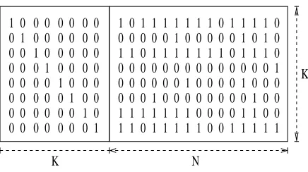
Fig. 3. The Systematic LT generator matrix

• If we have a generator matrixGK×N=[IK×K/AK×M],

whereI is an identity matrix having a size of [K ×

K] and A is a non-singular matrix having a size of

[K×M], then the PCM obeys the construction ofH =[AT_/I0_{], whereA}T _{is the transpose ofAandI}0_{is an}

identity matrix having a size of[M ×M][7], where N =K+M is the number of rows inGandKis the number of columns inG.

3. ANALYSIS OF SYSTEMATIC LUBY TRANSFORM CODES BASED ON EXIT CHARTS

Extrinsic Information Transfer (EXIT) charts [8] [9] were proposed by ten Brink and his collaborators. As mentioned in Section 2, systematic LT codes may be decoded by be-lief propagation. Hence, we can analyse systematic LT codes based on EXIT charts [8] [10]. Since systematic LT codes have a specific PCM construction, which contains the check bits in the corresponding rows and the message bits in the corresponding columns, while the second part of the PCM is constituted by a unity matrix having a size ofM ×M con-taining the check bits in both its rows and columns. Hence, we have to re-define the passing of the LLR messages during the systematic-LT decoding process as follows:

• The LLR messages are passed between the systematic LT message nodes and the systematic LT parity nodes.

Letdm represents the degree of the message nodes anddc

the degree of the parity nodes. Furthermore, letK denote the number of message nodes andN the number of variable nodes. Then the number of parity nodes is given byM=N-K. The degree distributionD(dc)of the check nodes is defined

as follows:

D(dc) =

      

0 ifdc= 1ordc >M_S,

1+S+ν

Z·M ifdc= 2,

PM−1

t=3 ( 1

t(t−1)+

S M ·

1

t) if3< dc < M, S

M ·log S

δ ifdc=

M S,

(4)

whereS,νwere defined in [2], We assume thatthe LT encod-ing process of [2] usencod-ing the ideal uniform random degree distribution is employed. Then the degree distribution of the message nodesD(dv)is defined as:

D[dm(dc)] = r, (5)

wherer= K_N is the code rate of the systematic LT code. Let us now consider the messages passed between the system-atic LT message nodes and the check nodes, when the LLR representation of the messages. LetQ0 as well asR0 denote the LLR information passed from the information nodes to the check nodes and that passed from the check nodes to the information nodes, respectively. The soft bit message corre-sponding toQ0is repeated here again

Q=tanh(Q 0

2 ). (6)

The extrinsic LLR information passing from the check nodes to the information nodes is defined by:

Q0 = dm−1

X

i=0

R0_i, (7)

where the initial soft channel-output message associated with the variable nodes is given by (R0₀=_N4

0 ·y) andydenotes the

output of an AWGN channel. Furthermore,R0_i, i = 1. . . dv−1

represents the LLR information arriving from the check nodes to the information nodes, except from that particular check node to which the LLR information messageQ0was sent. The extrinsic LLR informationR0passed from the check nodes to the information nodes is defined as:

tanh(R 0

2 ) = dc−1

Y

i=1

tanh(Q 0 i

2 ) ⇐⇒ R= d−1 Y

i=1

Ri, (8)

whereQ0

i,i=1,. . .,dc-1 represents the LLR information

arriv-ing from the information nodes, except from that particular information node to which the LLR information messageR0 was sent. LetmR,mR0 andmQdenote the mean ofR

0_,R0

0 andQ0. Then, from Equation (7) we have:

m(_Ql)=mR0+ (dm−1)·m

(l−1)

R , (9)

wherel is thel0thiteration and mR0 = 4· E

N0, while E is

the transmitted bit energy, while N0

2 is the one-side power spectral density of the noise. We assume thatR0 is Gaussian distributed. Hence,mRis can be updated according to:

m(_Rl)=J−1(I(X;R0(l))), (10) whereJ(mR)is defined as follows:

J(mR) =I(X;Rl) = (11)

=

Z ₁

√ 4πmR

e−

(l−mR)

From the equation used for calculating the mutual informa-tion in [11] we have:

I(X;R0) = 1

ln2 ∞

X

i= 1 1

2i(2i−1)[E(T

2i Q)]

dc−1_{, (12)}

where:

φi(mQ) = E(TR2i) (13)

=

Z +1

−1

2t(2i)

(1−t2₎p

4πmQ

e−(ln( 1+t

1−t)−mQ)

2

4mQ

dt.

Finally, we arrive at the required update formulae for the means mQandmRas follows:

m(_Ql) = mR0+ (dm−1)m

(l−1)

R (14)

m(_Rl) = J−1( 1

ln2 ∞

X

i=1

1

2i(2i−1)[E(T

2i mQl)]

dc−1_.(15)

Based on Equation (14) we arrive at the variable node’s EXIT function:

IEm = I(X;Q

0_{) =I(X;R}0

0, R01, . . . , R0dm−1) (16)

= f(I(X;R₀0), I(X;R0)) =f(Ich, IAm).

Similarly, from Equation (15) we derive the check node’s EXIT function as follows:

IEc = I(X;R

0_{) =I(X;Q}0

1, . . . , Q0dc−1) = (17)

= f(I(X;Q0)) =f(IAc) =

= 1

ln2 ∞

X

i=1

1

(2i−1)(2i)[φi(J −1_(I

Ac)]

dc−1_,

whereIch = I(X;R00)is the average channel output infor-mation,IAm = I(X;R

0_{)is the average a priori information}

at the input of the message node decoder andIEm is the

av-erage extrinsic information at the output of the message node decoder.

The systematic LT code has the degree distributionsD(dv)

andD(dc)formulated in Equations (4) and (5). Therefore,

the EXIT functions of the message and check nodes are given in Equations (16) and (17), which depend on the degrees of the message nodes and check nodes, respectively. Again, we assumed thatthe LT encoding process of [2] using the ideal uniform random degree distributionis employed. Hence, all the LT message nodes have the same degree, namely a de-gree ofdc−1. Finally, we arrive at the EXIT function of

the message nodes and the check nodes for the systematic LT code are expressed in the following form:

• Message node EXIT function:

IEm = f(Ich, IAm) (18)

= J(J−1(Ich+ (j−1)J−1(IAm));

• Check node EXIT function:

IEc =f(IAc) =

dc

X

j=2

dcjIEcj = (19)

= d_cmax

X

j=2 dc(j)·

1

ln2 ∞

X

i=1

( 1

2i(2i−1))[φi(J −1_(I

Ac)]

j−1

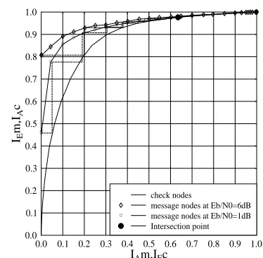
The EXIT chart of the systematic LT code is portrayed in Fig 4. The associated parameters are:

0.0 0.1 0.2 0.3 0.4 0.5 0.6 0.7 0.8 0.9 1.0

IAm,IEc

0.0 0.1 0.2 0.3 0.4 0.5 0.6 0.7 0.8 0.9 1.0

IE

m,I

A

c

check nodes

message nodes at Eb/N0=6dB message nodes at Eb/N0=1dB Intersection point

Fig. 4. EXIT chart of the systematic LT(1000,3000) code

• The check bits obey the same degree distribution as the LT packets, namely the Full Robust Soliton Distribu-tion (RSD) proposed in [2].

• All of the message bits have a degree of one.

• A total of 500 blocks are transmitted and each of them has 1000 bits. The rate of the systematic LT code was set tor= 1₃.

0.3 0.4 0.5 0.6 0.7 0.8 0.9 1.0 IAm,IEc

0.9 0.91 0.92 0.93 0.94 0.95 0.96 0.97 0.98 0.99 1.0

IE

m,I

A

c

check nodes

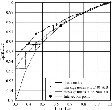
message nodes at Eb/N0=6dB message nodes at Eb/N0=1dB Intersection point

Fig. 5. Expanded view of the Systematic-LT(1000,3000) code’s EXIT chart

intersection between the message-node’s curve and the check-node’s curve, the systematic-LT decoder is unable to reach an infinitesimally low BER atEb/N0 = 1dB. By contrast, ob-serve in Fig. 5 that the systematic-LT decoder becomes capa-ble of converging to the (1,1) point atEb/N0= 6dBafter 10 iterations.

4. SIMULATION RESULTS

Fig. 6 shows the attainable performance of the systematic LT(1000,3000) code using the message-passing decoding tech-nique, when communicating over the AWGN channel, having an erasure probability ofPE=0. Fig 6 may be contrasted to

Fig 7, where transmission over the Wireless Internet associ-ated with differentEb/N0values andPe= 0.1is considered.

Fig. 8 shows the performance of the systematic LT code for transmission over the BEC having different erasure probabil-itiesPe, where the abscissa axis was scaled in terms of the

values of (1 −Pe). Again, the Robust Soliton degree

dis-tribution was used for the variable nodes of the systematic LT(1000,3000) code characterized in Fig. 6, Fig. 7 and Fig. 8. The degree distribution parameters of c=0.1 and δ = 0.5

were used as defined in [2]. We can see in Fig. 6 that for Pe=0 the BER becomes as low as10−5atEb/N0= 3.5dB. By contrast, when the erasure probability isPe=0.1, the decoder

reaches BER=10−5 atEb/N0= 4.5dB. The BER curves of the systematic LT code are significantly more smooth than for other combinations of LT codes and FEC codes [2]. The pro-posed scheme has the potential of maintaining a lower BER atEb/N0and that of tolerating higherPevalues than the

sys-tem of [2]. When we increase the length of the syssys-tematic-LT

0.5 1.0 1.5 2.0 2.5 3.0 3.5 4.0 4.5

Eb/No

10-5 10-4 10-3 10-2 10-1 1

BER

Systematic LT(1000,3000), AWGN channel, 0-iters Systematic LT(1000,3000), AWGN channel, 2-iters Systematic LT(1000,3000), AWGN channel, 4-iters Systematic LT(1000,3000), AWGN channel, 6-iters

Fig. 6. BER versus Eb/N0 performance of the systematic LT(1000,3000) code in AWGN channels using BPSK mod-ulation and no erasures

0.5 1.0 1.5 2.0 2.5 3.0 3.5 4.0 4.5 5.0 5.5 6.0

Eb/No

10-6 10-5 10-4 10-3 10-2 10-1 1

BER

BEC-AWGN, Pe=0.1, Systematic LT(1000,3000), 0-iters BEC-AWGN, Pe=0.1, Systematic LT(1000,3000), 2-iters BEC-AWGN, Pe=0.1, Systematic LT(1000,3000), 4-iters BEC-AWGN, Pe=0.1, Systematic LT(1000,3000), 6-iters

0.0 0.1 0.2 0.3 0.4 0.5 0.6 0.7 0.8 0.9 1.0

1-Pe

10-6 10-5 10-4 10-3 10-2 10-1 1

BER

Systematic LT(1000,3000), BEC channel, 0-iters Systematic LT(1000,3000), BEC channel, 2-iters Systematic LT(1000,3000), BEC channel, 4-iters Systematic LT(1000,3000), BEC channel, 6-iters

Fig. 8. BER versus1−Pe performance of the systematic

LT(1000,3000) code in the noiseless BEC channel

0.5 1.0 1.5 2.0 2.5 3.0 3.5 4.0 4.5

Eb/No

10-6 10-5 10-4 10-3 10-2 10-1 1

BER

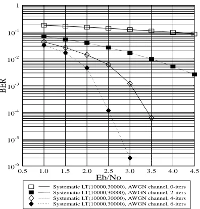
Systematic LT(10000,30000), AWGN channel, 0-iters Systematic LT(10000,30000), AWGN channel, 2-iters Systematic LT(10000,30000), AWGN channel, 4-iters Systematic LT(10000,30000), AWGN channel, 6-iters

Fig. 9. BER versus Eb/N0 performance of the system-atic LT(10000,30000) for transmission over the AWGN-contaminated BEC associated withPe= 0

codes, their performance is improved, as seen in Fig. 9. More specifically, a BER of 10−5 may be attained at Eb/N0 =

3.0dBafter 6 iterations of the systematic-LT decoder. Finally, observe in Fig 8 that the systematic LT decoder is capable of maintaining an infinitesimally low BER for erasure probabil-ities as high asPe= 0.4in the BEC.

5. CONCLUSIONS

The concept of systematic LT codes was introduced with the aid of appropriately modifying the robust soliton degree dis-tribution of [2]. The systematic LT coding concept facilitated the employment of the classic belief-propagation based soft decoding of the resultant systematic LT codes. The main ben-efit of the proposed scheme is that it is capable of mitigat-ing the effects of catastrophic error propagation across the LT-encoded packets. Our future work will consider the em-ployment of diverse classic FEC codes in the context of soft-decoded LT codes for the sake of improving the associated performance versus complexity as well as versus code-rate trade-offs.

6. REFERENCES

[1] M. Luby, “LT codes,” inProceeding of the 43rd Annual IEEE Sympo-sium on Foundations of Computer Science, November 2002, pp. 271– 282.

[2] R. Tee, T.D. Nguyen, L-L. Yang and L. Hanzo., “Serially Concatenated Luby Transform Coding and Bit-Interleaved Coded Modulation Using Iterative Decoding for the Wireless Internet,”Proceedings of VTC 2006 Spring, Melbourne,CD ROM,, vol. 138, no. 4, pp. 177–182, May 2006. [3] T. Stockhammer H. Jenkac, T. Mayer and W. Xu, “Soft decoding of lt-codes for wireless broadcast,”in Proc. IST Mobile, Dresden, Germany, 2005.

[4] R. Palanki, J.S. Yedidia., “Rateless codes on noisy channels,” ISIT 2004. Proceedings, p. 37, June 2004.

[5] T. J. Richardson and R. L. Urbanke, “The capacity of low density parity check codes under message-passing decoding,”IEEE Transactions on Information Theory, pp. 599–618, Feb 2001.

[6] S. Y. Chung, “On the construction of some capacity-approaching cod-ing schemes,”Ph.D thesis, MIT, USA, 2000.

[7] R. Gallager, “Low Density Parity Check Codes,”IRE Transactions On Information Theory, 1962.

[8] S. ten Brink, “Convergence behavior of iteratively decoded parallel concatenated codes,”Communications, IEEE Transactions, 2001. [9] G. Kramer A. Ashikhmin and S. ten Brink, “Extrinsic information

transfer functions: model and erasure channel properties,”Information Theory, IEEE Transactions, 2004.

[10] E. Sharon, “Analysis of belief-propagation decoding of ldpc codes over the biawgn channel using improved gaussian approximation based on the mutual information measure,”Electrical and Electronics Engineers in Israel. The 22nd Convention of, 2002.