Chapter 5
Control runs
5.1
Introduction
Three coupled model control runs are presented in this chapter; these are sum-marised in Table 5.1. They differ from each another only in the initial states of the ocean and atmosphere models, and in the spatial and temporal distribution of the flux adjustments which are applied. Each run represents a control simulation for pre-industrial conditions, consistent with PMIP2 (Paleoclimate Modelling Inter-comparison Project, 2005) experimental design. The atmospheric carbon dioxide concentration is held constant at 280 ppm, while present-day values are used for the Earth’s orbital parameters. Further details regarding the experimental design are provided in Appendix A.
Run CON-DEF represents the default coupled model simulation. The initial states of the atmosphere and ocean models are provided by the final states of spin-up runs A-DEF (Section 2.3.1) and O-DEF (Section 2.3.2) respectively. The model is integrated for 1400 years, with flux adjustments (Section 2.6) being applied. The drift in the mean climate state is examined in Section 5.2, and the nature of the internal variability is examined in Section 5.3.
Run CON-SHF was initialised from the final state of ocean model run O-SHF, for which the prescribed surface tracers were shifted forward in time by one month relative to observations (Section 4.3), while run CON-EFF was initialised from the final state of ocean model run O-EFF, for which effective surface tracers were em-ployed (Section 4.4). Each run is integrated for 1100 years. The climates of these
Name Spin-up runs Flux
Ocean Atmosphere adjustments
CON-DEF O-DEF A-DEF O-DEF/A-DEF
CON-SHF O-SHF A-SHF O-SHF/A-SHF
CON-EFF O-EFF A-EFF O-EFF/A-EFF
Table 5.1: Control runs conducted using the Mk3L coupled model: the name used herein, the names of the ocean and atmosphere model spin-up runs, and the spin-up runs from which the flux adjustments were derived.
two runs are contrasted with that of run CON-DEF in Section 5.4.
5.2
Climate drift
5.2.1 Atmosphere
Surface air temperature
The evolution of the simulated global-mean and zonal-mean surface air temperature (SAT) during run CON-DEF is shown in Figure 5.1. The global-mean SAT is very stable, cooling just 0.23◦C by the final century of the run. The mean changes over land and the ocean are similar, with cooling of 0.28◦C and 0.21◦C respectively by the final century. The zonal-mean SAT exhibits negligible drift at most latitudes. Cooling at∼60◦N, and warming at∼80◦N, occur during the first century of the run, but the temperatures at these latitudes stabilise thereafter. Only at high latitudes in the Southern Hemisphere is there an ongoing trend, with the zonal-mean SAT warming slightly at first, but then cooling as the run progresses.
Figure 5.2 shows the change in SAT, between the atmosphere model spin-up run and the final century of run CON-DEF. The stability of the simulated surface air temperature is apparent, with the annual-mean SAT drifting by less than 1◦C over 97% of the Earth’s surface. The root-mean-square difference in the annual-mean surface air temperature, between the atmosphere model spin-up run and the final century of run CON-DEF, is just 0.53◦C. The drift in the zonal-mean SAT at high latitudes in the Northern Hemisphere can be seen to arise from a reduction in winter temperatures in the Barents Sea, the Sea of Okhotsk and Hudson Bay, and from a warming in the Greenland Sea.
Sea ice
Figure 5.3 shows the evolution of the sea ice extent and volume in each hemisphere during run CON-DEF. After some initial adjustment, the Northern Hemisphere sea ice extent is highly stable; the mean extent for the final century of the run is 12.1×10¹²
m2
, 16% greater than for the atmosphere model spin-up run. Consistent with the cooling trend at high southern latitudes, the sea ice extent in the Southern Hemisphere exhibits a slight upwards trend. The mean extent for the final century is 13.4×10¹²
m2
, 7% greater than for the atmosphere model spin-up run.
The sea ice volumes in each hemisphere exhibit similar behaviour to the sea ice extent. The Northern Hemisphere ice volume exhibits some initial adjustment, but is then stable; the mean volume for the final century of the run is 13.1×10¹²
m3
, 29% greater than for the atmosphere model spin-up run. The Southern Hemisphere sea ice volume exhibits a slight upwards trend; the mean volume for the final century is 5.6×10¹²
m3
, 8% greater than for the spin-up run.
5.2. CLIMATE DRIFT 153
5.2. CLIMATE DRIFT 155
where there has been a change in the surface air temperature.
In the Northern Hemisphere, these changes consist of an expansion in the ice cover in the Barents Sea and the Sea of Okhotsk, with the sea ice also now extending into Hudson Bay and the Labrador Sea. This accounts for the increase in sea ice extent relative to the atmosphere model spin-up run, and brings the model into significantly better agreement with observations. Sea ice formation is also simulated in the northern Caspian Sea, again in agreement with observations; however, this ice persists throughout the summer, which the observed cover does not. In contrast to these increases in ice extent, there is also a reduction in the sea ice cover in the Greenland Sea. In the Southern Hemisphere, there is an increase in the simulated winter ice extent, combined with a slight reduction in the summer ice cover.
Figure 5.5 shows the average sea ice thicknesses for the final century of the run. Comparison with Figure 2.12, which shows the climatology of the atmosphere model spin-up run, indicates that the ice thicknesses are very consistent between the stand-alone atmosphere model and the coupled model. The sea ice which forms in Hudson Bay is significantly thicker than that which forms elsewhere, however, and reaches the model’s upper limit of 6 m (Section 2.2.1) during winter.
5.2.2 Ocean
Sea surface temperature and salinity
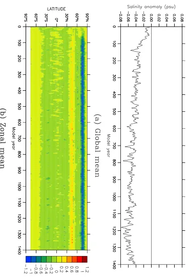
The evolution of the simulated global-mean and zonal-mean sea surface temperature (SST) and sea surface salinity (SSS) during run CON-DEF are shown in Figures 5.6 and 5.7 respectively. The drift in the simulated SST is similar to that in the sim-ulated surface air temperature. The global-mean SST is very stable, cooling just 0.15◦C by the final century of the run, while the zonal-mean SST exhibits an ini-tial cooling at ∼60◦N, and a warming at ∼80◦N, but with little subsequent drift at these latitudes thereafter. As with the surface air temperature, there is also an initial warming in the Southern Ocean, followed by a slight cooling trend. The sim-ulated SSS is very stable, with the global mean freshening just 0.053 psu by the final century of the run. The zonal-mean SSS exhibits an initial freshening at ∼75◦N, and a slight upward trend at∼45◦N, but otherwise experiences little drift.
Figure 5.8 shows the change in SST between the ocean model spin-up run, and the final century of run CON-DEF. The stability of the simulated sea surface tem-perature is apparent, with the annual-mean SST drifting by less than 0.5◦C over 95% of the surface of the ocean. The root-mean-square difference, between the ocean model spin-up run and the final century of run CON-DEF, is just 0.30◦C. As with the surface air temperature, the largest drift occurs at high latitudes, particularly in the Northern Hemisphere; it therefore appears to be related to the changes in sea ice extent. The strongest cooling occurs in Hudson Bay, the Sea of Okhotsk, the Barents Sea, and along the Atlantic coast of Canada; these are the regions where the sea ice cover has expanded relative to the atmosphere model spin-up run. Slight warming is apparent at isolated locations in the North Atlantic, Arctic and Southern Oceans.
5.2. CLIMATE DRIFT 157
5.2. CLIMATE DRIFT 159
5.2. CLIMATE DRIFT 161
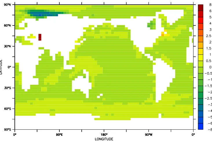
Figure 5.9: The annual-mean sea surface salinity (psu) for years 1301–1400 of cou-pled model run CON-DEF, expressed as an anomaly relative to the annual-mean sea surface salinity for the final 100 years of ocean model spin-up run O-DEF.
sea surface salinity is apparent, with the annual-mean SSS drifting by less than 0.5 psu over 99% of the surface of the ocean, and with the root-mean square change being just 0.35 psu. Excluding the inland seas, the only significant changes are a freshening in the Barents Sea and a slight increase in the SSS along the Atlantic coast of Canada, where there has been in increase in the simulated sea ice cover.
The largest salinity drift occurs in the Caspian Sea, where the mean SSS has increased by 6.7 psu by the final century of the run. This is the only ocean basin which is not connected to the world ocean within the Mk3L ocean model (Phipps, 2006). The flux adjustments which are applied within the coupled model are time-invariant, and any changes in the fluxes of freshwater into the Caspian Sea relative to the atmosphere model spin-up run, be they changes in the fluxes of precipitation, evaporation or run-off, will therefore result in a drift in the mean salinity.
The other inland seas do not exhibit a drift of the magnitude of that exhibited by the Caspian Sea; this suggests that the parameterised mixing across unresolved straits within the Mk3L ocean model (Phipps, 2006) is successful at representing the effects of the exchange of water between these bodies and the world ocean.
Water properties
The evolution of the simulated global-mean potential temperature, salinity and po-tential density of the world ocean, and of the simulated global-mean vertical profiles, during run CON-DEF are shown in Figures 5.10, 5.11 and 5.12 respectively.
5.2. CLIMATE DRIFT 163
5.2. CLIMATE DRIFT 165
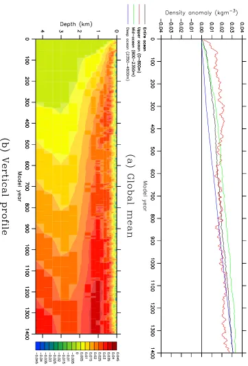
Figure 5.12: The drift in annual-mean σθ (kgm−
3
) during coupled model run CON-DEF: (a) the global means for the entire ocean (black), upper ocean (red, 0–800 m), mid-ocean (green, 800–2350 m) and deep ocean (dark blue, 2350–4600 m), and (b) the global-mean vertical profile. The values shown are five-year running means, and are expressed as anomalies relative to the annual-meanσθ for the final 100 years of
0.23◦C by year 1400. The temperature of the upper ocean exhibits greater inter-annual variability than either the mid- or deep ocean, reflecting the attentuation of variability on interannual timescales with depth. There is an ongoing cooling trend at all depths, with the strongest cooling of 0.33◦C occurring at a depth of 410 m. The evolution of the zonal-mean potential temperature during run CON-DEF is shown in Figure 5.13; the cooling can be seen to propagate outwards from a region located in the upper ocean at ∼50◦N. This can be attributed to a decrease in the temperature of North Atlantic Deep Water, arising from a cooling of the surface waters in the North Atlantic (Figure 5.8). Although there is also a warming of the Arctic Ocean at depth, this appears to have stabilised by year 1000.
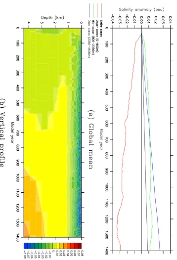
Drift in the mean salinity of the ocean is also small, with an increase of just 0.008 psu during the 1400 years of run CON-DEF. However, this increase cannot be accounted for by the increase in sea ice volume relative to the atmosphere model spin-up run. The increase of 3.4×10¹²
m3
in the ice volume represents an input of salt to the world ocean of ∼8.4×10¹⁰
m3
, which is equivalent to an increase in the mean salinity of just∼6.6×10⁻⁵
psu.
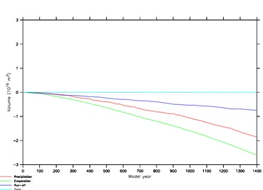
Neither can the drift be attributed to changes in any of the reservoirs of freshwa-ter within the climate system. The increase in the mean salinity is equivalent to a net freshwater flux of∼3.2×10¹⁴
m3
out of the ocean; normalised by the surface area of the Earth, this flux is equivalent to a depth of freshwater of∼0.6 m. Figure 5.14 shows the temporal integrals of the changes in the fluxes of precipitation, evapora-tion and run-off into the world ocean, relative to the atmosphere model spin-up run A-DEF. By year 1400, the changes amount to a net freshwater flux into the ocean of just 7×10¹¹
m3
. The salinity drift therefore appears to represent a conservation error within the model, and requires further investigation.
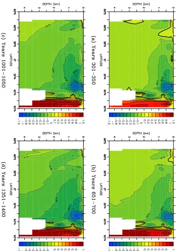
Figure 5.15 shows the evolution of the zonal-mean salinity during run CON-DEF. There is a vertical redistribution of salt, with freshening of the surface layers and an increase in the salinity of the deep ocean. The salinity of the deep Arctic Ocean appears to have stabilised by year 1000, with the ongoing increase in the salinity of the deep ocean appearing to arise instead from a slight increase in the salinity of the deep Southern Ocean.
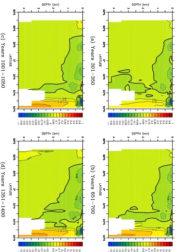
As a result of the minimal drift in the potential temperature and salinity of the world ocean, the potential density is also very temporally stable. The increase in the mean density by year 1400 is just 0.031 kgm−3; apart from a slight increase in the buoyancy of the surface layers, arising from the freshening of the upper ocean, the increase in density is relatively uniformly distributed throughout the water column. Figure 5.16 shows the evolution of the zonal-mean potential density during run CON-DEF. There is a slight increase in the density of the deep Arctic Ocean, but otherwise the zonal-mean potential density is stable to within 0.05 kgm−3 throughout the mid-and deep ocean.
Circulation
5.2. CLIMATE DRIFT 167
Figure 5.14: The changes in the freshwater fluxes into the world ocean during run CON-DEF: the temporal integrals of the changes in the fluxes of precipitation (red), evaporation (green), run-off (dark blue), and the total freshwater flux (light blue). Changes are expressed relative to the final 40 years of the atmosphere model spin-up run A-DEF.
the mean rates of NADW and AABW formation for the final century of the run are 13.8 and 11.2 Sv respectively. These figures represent slight increases on the rates of 13.6 and 9.5 Sv, respectively, for the final century of ocean model spin-up run O-DEF. The strength of the Antarctic Circumpolar Current exhibits only a very slight upward trend during the course of the run. The mean strength for the final century is 148.1 Sv, only slightly stronger than the mean strength of 145.3 Sv for the final century of ocean model spin-up run O-DEF.
The mean meridional overturning streamfunctions for the final century of the run are shown in Figure 5.18; they can be compared with those diagnosed from the final century of ocean model spin-up run O-DEF (Figure 2.17). The intensification in the rate of Antarctic Bottom Water formation within the coupled model is apparent.
Mean sea level
The Mk3L ocean model employs the rigid-lid approximation (Section 2.2.2), and hence cannot directly simulate any change in sea level. However, it is possible to infer thestericsea level change, being that which arises from changes in the density of the ocean. By assuming that the mass of water within each gridbox remains constant, then a volume change can be inferred from any change in the density of its contents. Let the gridbox (i, j, k) have mass Mi,j,k, and let the density and
5.2. CLIMATE DRIFT 169
Figure 5.16: The zonal-mean σθ (kgm−3) for coupled model run CON-DEF,
ex-pressed as an anomaly relative to the average σθ for the final 100 years of ocean
5.2. CLIMATE DRIFT 171
5.2. CLIMATE DRIFT 173
the relation
ρi,j,k(0)Vi,j,k(0) =ρi,j,k(t)Vi,j,k(t) =Mi,j,k (5.1)
which, upon re-arrangement, gives
Vi,j,k(t) =
Mi,j,k
ρi,j,k(t)
(5.2)
= ρi,j,k(0)
ρi,j,k(t)
Vi,j,k(0) (5.3)
The change in the volume of the gridbox, ∆Vi,j,k(t), is therefore given by
∆Vi,j,k(t) = Vi,j,k(t)−Vi,j,k(0) (5.4)
= ρi,j,k(0)
ρi,j,k(t) −
1 !
Vi,j,k(0) (5.5)
The change in mean sea levelH(t) is obtained by summing these volume changes over all the ocean gridboxes, and then dividing the total change in the volume of the ocean by the surface area A, thus:
H(t) = 1
A X i X j X k
ρi,j,k(0)
ρi,j,k(t) −
1 !
Vi,j,k(0) (5.6)
Equation 5.6 can be used to infer the evolution of the mean sea level during a coupled model simulation. Using the International Equation of State of Seawater 1980 (UNESCO, 1981), as described by Fofonoff (1985), to calculate density, and using the final century of ocean model spin-up run O-DEF as the reference state, Figure 5.19 shows the changes in the mean sea level inferred from run CON-DEF. The cooling of the world ocean causes it to contract slightly, with a drop of 14.2 cm in the mean sea level by year 1400.
5.2.3 Summary
The control climate of the Mk3L coupled model exhibits a very high degree of stability. Over the course of a 1400-year control simulation, the global-mean sur-face air temperature cools 0.23◦C, representing an average rate of change of just -0.016◦C/century. Some initial adjustment occurs during the first century of the run, during which there is an expansion in the Northern Hemisphere sea ice cover. The resulting cooling in the North Atlantic results in a decrease in the temperature of North Atlantic Deep Water, which leads to a slow but ongoing cooling of the ocean. The thermohaline circulation strengthens slightly during the first century of the run, but is stable thereafter.
Figure 5.19: The steric change in mean sea level diagnosed from coupled model run CON-DEF.
the sea surface temperatures used to spin-up the atmosphere model appear to be too warm in the Hudson Bay region, and that this leads to deficient sea ice cover. If realistic ice cover could be achieved within the stand-alone atmosphere model, it is possible that the initial adjustment within the coupled model would not occur. The cooling in the North Atlantic, and hence in the ocean, could therefore be averted.
It should be noted, however, that the cooling trend is much smaller that that exhibited by the majority of coupled general circulation models (Bell et al., 2000; Lambert and Boer, 2001). Table 5.2 shows the rate of drift in global-mean surface air temperature, as exhibited by 15 models which participated in the Coupled Model Intercomparison Project (Lambert and Boer, 2001, Table 7). The drift exhibited by Mk3L is less, typically by between one and two orders of magnitude, than that exhibited by all seven of the non-flux adjusted models, and by all but one of the eight models which employed flux adjustments.
Only the CSIRO Mk2 coupled model exhibits a lower rate of drift; the stability of the control climate of this model has been noted in other studies (e.g.Hirst et al., 2000;Bi et al., 2001;Bi, 2002;Hunt, 2004). The drift exhibited by the CSIRO Mk3 coupled model, which does not employ flux adjustments, is much larger, however, with Gordon et al. (2002) finding that the global-mean sea surface temperature declines ∼0.5◦C over the course of an 80-year control simulation.
5.3. CLIMATE VARIABILITY 175
Model Trend in global-mean
SAT (◦C/century)
Flux adjusted
CCCma +0.240
CCSR +0.735
CSIRO -0.009
GFDL +0.197
MPI E3/L +0.188
MPI E4/O -0.124
MRI +1.057
UKMO +0.030
Non-flux adjusted
CERFACS +0.553
COLA +0.352
GISS MILL +0.929
GISS RUSS +0.702
LMD +4.206
NCAR CSM -0.211
[image:25.595.224.427.107.372.2]NCAR WM +0.892
Table 5.2: The rate of drift in global-mean surface air temperature (SAT) for 15 coupled general circulation models which participated in the Coupled Model Inter-comparison Project (Lambert and Boer, 2001). Both flux adjusted and non-flux adjusted models are shown.
An apparent freshwater conservation error has also been identified within the Mk3L coupled model, which requires further investigation.
5.3
Climate variability
5.3.1 Interannual variability
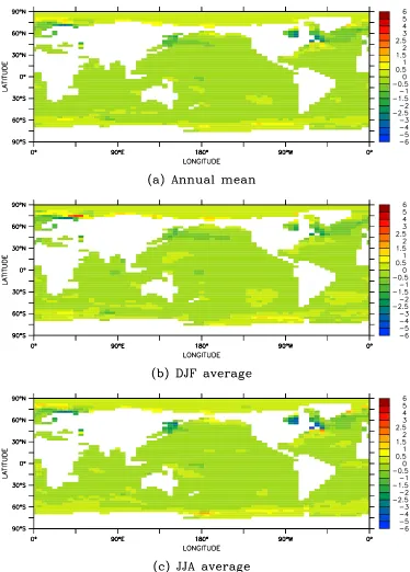
Figure 5.20 shows the standard deviations in the annual-mean surface air tempera-ture (SAT), sea surface temperatempera-ture (SST) and sea surface salinity (SSS), for years 101–1400 of run CON-DEF. Note that the first 100 years of the run have been ex-cluded, in order to allow for any initial adjustment, and that the data has been de-trended through the application of a high-pass filter. This filter was used to remove variability on timescales longer than 100 years, and hence to remove the effects of any drift in the model climate.
Variability in the annual-mean SAT is greatest over the high-latitude oceans, re-flecting interannual variability in the sea ice cover. At mid-latitudes, the variability is greater over land than over the ocean, reflecting the differing surface heat capac-ities, while, in the tropics, the interannual variability is greatest over the central Pacific Ocean.
5.3. CLIMATE VARIABILITY 177
along the edge of the Northern Hemisphere sea ice zone, again reflecting interannual variability in the sea ice cover. However, as a result of the insulating effects of sea ice, variability in the annual-mean SST is otherwise small at high latitudes. The Pacific Ocean exhibits the greatest variability at low latitudes, with the largest standard deviation of 0.66◦C occurring in the central Pacific; this indicates the presence of a simulated El Ni˜no-Southern Oscillation (see below). Overall, the annual-mean SST exhibits less variability than the annual-mean SAT, with the area-weighted global-mean standard deviations being 0.30◦C and 0.45◦C respectively.
Variability in the annual-mean SSS (Figure 5.20c) is dominated by two pro-cesses. The largest variability occurs over the Arctic Ocean and along the Atlantic coast of Canada, reflecting interannual variability in the sea ice cover. At lower lat-itudes, however, the greatest variability occurs in the monsoonal regions, reflecting interannual variability in the strength and position of the monsoons.
Figure 5.21 shows the leading principal components (Wilks, 1995) of the annual-mean surface air temperature, sea surface temperature and sea surface salinity for years 101–1400 of run CON-DEF. As with the standard deviations, the first 100 years of the run have been excluded from the analysis and, prior to calculating the principal components, a high-pass filter was applied in order to remove variability on timescales longer than 100 years. The fractions of the total variance to be described by the leading principal components are 10.6%, 22.3% and 18.1%, for the SAT, SST and SSS respectively. In contrast, the second principal components describe 5.5%, 6.0% and 8.1% respectively.
In the case of the SST, the leading mode of variability is therefore dominant to an extent not encountered in the case of either the SAT or SSS. The spatial pattern shown in Figure 5.21b is associated with a time-dependent amplitude, which indi-cates both the strength and the phase of the mode. The positive phase consists of positive anomalies in the eastern tropical Pacific Ocean, with the largest anomalies occurring over the equator near 160◦W. These are accompanied by negative anoma-lies to the west and at higher latitudes, with the largest anomaanoma-lies occurring in the central northern Pacific Ocean, at ∼160◦W, ∼35◦N. In the negative phase of this mode, the signs of the anomalies are reversed.
The leading mode of variability in the annual-mean surface air temperature, while representing a smaller fraction of the total variance, clearly represents the same physical mode. Positive and negative temperature anomalies over the Pacific Ocean exhibit the same spatial structure as for the SST. However, there is also associated variability at higher latitudes, with temperature anomalies over the Ross Sea, Hudson Bay, and the eastern United States, which exceed in magnitude those over the Pacific Ocean.
5.3. CLIMATE VARIABILITY 179
5.3.2 El Ni˜no-Southern Oscillation
The leading mode of variability in the annual-mean sea surface temperature ex-hibits the same spatial structure in the Pacific Ocean as the temperature anomalies which occur during El Ni˜no events. The El Ni˜no-Southern Oscillation (ENSO) phe-nomenon (e.g.Philander, 1990) represents the dominant mode of internal variability within the coupled atmosphere-ocean system, and is one of the largest sources of interannual climate variability.
An El Ni˜no event occurs when mean sea level pressure (MSLP) decreases over the central and eastern tropical Pacific Ocean. As a result, the easterly trade winds weaken, and the warmer waters of the western tropical Pacific Ocean migrate east-wards. An El Ni˜no event is therefore characterised by positive (negative) SST (MSLP) anomalies in the eastern tropical Pacific Ocean, and negative (positive) SST (MSLP) anomalies in the western tropical Pacific Ocean. A La Ni˜na event represents the opposite phase, with negative (positive) SST (MSLP) anomalies in the east, and positive (negative) SST (MSLP) anomalies in the west.
Trenberth (1997) defines an El Ni˜no event as one where the five-month running mean of the SST anomalies in the Ni˜no 3.4 region (170◦–120◦W, 5◦S–5◦N) exceeds 0.4◦C for at least six consecutive months. The Ni˜no 3.4 SST anomalies are derived from years 101–1400 of run CON-DEF, through the application of a high-pass fil-ter which removes variability on timescales longer than 100 years. The standard deviation of the five-month running mean of the simulated anomalies is 0.49◦C, as compared to the observed value for the period 1950–1979 of 0.71◦C (Trenberth, 1997).
While the Ni˜no 3.4 SST anomaly is a measure of the oceanic changes associated with ENSO, the Southern Oscillation Index (SOI, e.g. Ropelewski and Jones, 1987) is a measure of the atmospheric changes. The SOI represents the standardised anomaly of the MSLP difference between Tahiti (149.6◦W, 17.5◦S) and Darwin (130.9◦E, 12.5◦S). LetPi be the MSLP difference (Tahiti minus Darwin) for calendar month i, let Pi be the long-term mean of Pi, and let σi be the long-term standard
deviation of Pi. The SOI is therefore given by
SOI = 10 Pi−Pi
σi
!
(5.7)
The factor of 10 is included by convention. Negative values of the SOI represent positive MSLP anomalies in the western tropical Pacific Ocean, and negative MSLP anomalies in the eastern tropical Pacific Ocean, as occur during an El Ni˜no event. Values of the SOI are diagnosed from years 101–1400 of run CON-DEF, with the MSLP anomalies Pi−Pi being calculated through the application of a high-pass
filter which removes variability on timescales longer than 100 years.
The Ni˜no 3.4 SST anomaly and Southern Oscillation Index are strongly anti-correlated, with a correlation coefficient of -0.78. This is illustrated by Figure 5.22, which shows the values of the two indices for years 101–200 of run CON-DEF.
5.3. CLIMATE VARIABILITY 181
throughout the western Pacific Ocean. The maximum anti-correlation of -0.77 oc-curs at 163◦W, 2◦N, within the Ni˜no 3.4 region. The spatial structure of the correla-tions strongly resembles that of the leading principal component of the annual-mean SST (Figure 5.21b).
Applying the definition of Trenberth (1997), there are 166 simulated El Ni˜no events during years 101–1400 of run CON-DEF, with an average return period of 7.8±0.5 years (note that the errors quoted in this section represent one standard deviation in the mean). The average duration of the events is 17.4±0.8 months, and the average magnitude of the events, defined here as the maximum size of the Ni˜no 3.4 SST anomaly, is 0.88±0.02◦C. Using observed sea surface temperatures for the period January 1950–March 1997, Trenberth (1997) identifies 15 El Ni˜no events, giving an observed return period of ∼3.2 years. The average duration of these events is 11.8 months, and the average magnitude is ∼1.3◦C. Thus, relative to observations, the simulated frequency is too low, and the simulated El Ni˜no events are too long and too weak.
Figure 5.23 shows the power spectra of the simulated Ni˜no 3.4 SST anomaly and Southern Oscillation Index, and of the amplitude of the leading principal component of the annual-mean SST; note that variability on timescales longer than 100 years was removed from the original data through the application of a high-pass filter. Note also that the spectra have been smoothed through the application of a Hann window (Press et al., 1992) of width 25, which corresponds to a width of ∼0.019 years−1
in frequency units. A Hann window is defined by the function
wj =
1 2
1−cos 2πj
N
(5.8)
If no smoothing is applied, the standard deviation in each value is ±100%; however, the application of a smoother of width N reduces the standard deviation by a factor of √N (Wilks, 1995). A Hann window of width N has an effective width of ∼ 12N (Press et al., 1992), and so the standard deviation in each value in
Figure 5.23 is ∼ ±28%.
Apparent from Figure 5.23 is the strong correlation between the power spec-tra for the Ni˜no 3.4 SST anomaly and the leading principal component of annual-mean SST. Interdecadal variability can be seen to dominate, with peaks at ∼0.028 years−1
and ∼0.048 years−1
, corresponding to periods of∼35 years and ∼21 years respectively. Thus there is strong interdecadal modulation of the simulated El Ni˜no-Southern Oscillation, consistent with the ENSO-like interdecadal variability observed in the Pacific Ocean (Zhang et al., 1997;Lohmann and Latif, 2005). Such interdecadal variability is also exhibited by the CSIRO Mk2 coupled model (Walland et al., 2000;Vimont et al., 2002).
Figure 5.23: The normalised power spectra of the Ni˜no 3.4 sea surface temper-ature anomaly (red), the Southern Oscillation Index (green), and the amplitude of the leading principal component of annual-mean sea surface temperature (dark blue), for years 101–1400 of coupled model run CON-DEF. Each spectrum has been normalised so that the total power is equal to 1, and then smoothed through the application of a Hann window of width 25.
5.3.3 Summary
The dominant mode of internal variability has been shown to exhibit the same spatial structure and correlations as the observed El Ni˜no-Southern Oscillation phe-nomenon. The frequency is too low, however, and the simulated El Ni˜no events are too long and too weak. There is also excessive modulation on interdecadal timescales.
The strength of the simulated ENSO, as defined by the standard deviation of the Ni˜no 3.4 SST anomalies, is typical of low-resolution coupled models, such as those which participated in the Coupled Model Intercomparison Project (AchutaRao and Sperber, 2002); many of these models also failed to correctly simulate the observed frequency. However, higher-resolution coupled models, such as those which con-tributed to the IPCC Fourth Assessment Report, have a much more realistic ENSO (Guilyardi, 2006).
5.4. THE IMPACT OF THE SPIN-UP PROCEDURE 183
CON-DEF CON-SHF CON-EFF
Change in global-mean -0.21 -0.31 -0.45
SAT (◦C)
RMS change in annual- 0.52 0.68 0.82
mean SAT (◦C)
Sea ice extent NH 12.0 12.5 13.2
(1012 m2
) SH 13.3 14.1 15.6
Sea ice volume NH 12.5 14.7 16.4
(1012 m3
) SH 5.5 6.1 6.4
Table 5.3: Some statistics for years 1001–1100 of coupled model runs CON-DEF, CON-SHF and CON-EFF: the change in global-mean surface air temperature (SAT), relative to the atmosphere model spin-up runs; the root-mean-square (RMS) change in the SAT; and the sea ice extents and volumes for each hemisphere.
of the simulated El Ni˜no. However, the CSIRO Mk3 coupled model, which employs a much higher spatial resolution than Mk3L, is successful at capturing both the magnitude and frequency of the observed ENSO phenomenon (Gordon et al., 2002; Cai et al., 2003; Guilyardi, 2006).
5.4
The impact of the spin-up procedure
5.4.1 Climate drift: atmosphere
Some statistics on the drift in the climate of the atmosphere model during coupled model control runs CON-SHF and CON-EFF are shown in Table 5.3; statistics are also provided for the equivalent period of run CON-DEF. The nature of the drift is discussed in the following section.
Surface air temperature
The evolution of the simulated global-mean and zonal-mean surface air temperature (SAT) during runs CON-SHF and CON-EFF is shown in Figure 5.24. While the global-mean SAT exhibits only a slight downward trend for both runs, the rate of cooling is greater than for run CON-DEF. The evolution of the zonal-mean SAT is similar to run CON-DEF for both runs, with an initial cooling at∼60◦N, an initial warming at ∼80◦N, and an ongoing cooling trend at ∼60◦S. However, while the cooling at∼60◦N stabilises during the initial centuries of run CON-SHF, it appears to represent an ongoing trend in run CON-EFF. The cooling trend at∼60◦S in run CON-EFF is also stronger than in either of runs CON-DEF or CON-SHF.
5.4. THE IMPACT OF THE SPIN-UP PROCEDURE 185
Sea ice
Figure 5.25 shows the evolution of the sea ice extent and volume in each hemisphere, for runs CON-SHF and CON-EFF. Both runs experience an increase in Northern Hemisphere sea ice extent during the initial centuries; the extent stabilises thereafter in run CON-SHF, but exhibits a slight upward trend in run CON-EFF. Consistent with the cooling trends over the Southern Ocean, both runs experience an upward trend in sea ice extent in the Southern Hemisphere, although the trend is only slight in the case of run CON-SHF.
The sea ice volume in each hemisphere varies in a similar manner to the sea ice extent. After some initial adjustment, the Northern Hemisphere ice volume is stable in run CON-SHF, but exhibits a slight upward trend in run CON-EFF. The Southern Hemisphere ice volume exhibits a slight upward trend in both runs.
The changes in sea ice extent are similar to those within run CON-DEF, with the ice cover expanding into Hudson Bay, the Labrador Sea and the Caspian Sea, an increase in ice cover in the Barents Sea and the Sea of Okhotsk, and a decrease in cover in the Greenland Sea (not shown). In run CON-SHF, ice persists throughout the summer in the Gulf of St Lawrence (on the Atlantic coast of Canada), while in run CON-EFF, the sea ice concentrations in Hudson Bay are higher than for run CON-DEF.
Relative to run CON-DEF, there is little difference in the ice thicknesses exhib-ited by runs CON-SHF and CON-EFF (not shown). However, the model’s upper limit of 6 m is reached by both runs over the Caspian Sea, indicating the degree to which this basin has cooled.
5.4.2 Climate drift: ocean
Some statistics on the drift in the climate of the ocean model during coupled model control runs CON-SHF and CON-EFF are shown in Table 5.4; statistics are also provided for the equivalent period of run CON-DEF. The nature of the drift is discussed in the following section.
Sea surface temperature and salinity
Figures 5.26 and 5.27 show the evolution of the simulated global-mean and zonal-mean sea surface temperature (SST) and sea surface salinity (SSS), respectively, for runs CON-SHF and CON-EFF.
5.4. THE IMPACT OF THE SPIN-UP PROCEDURE 187
5.4. THE IMPACT OF THE SPIN-UP PROCEDURE 189
CON-DEF CON-SHF CON-EFF
Change in global-mean SST -0.14 -0.20 -0.31
(◦C)
Change in global-mean SSS -0.053 -0.093 -0.034
(psu)
RMS change in annual-mean 0.31 0.38 0.47
SST (◦C)
RMS change in annual-mean 0.33 0.31 0.23
SSS (psu)
Change in mean potential -0.18 -0.30 -0.39
temperature (◦C)
Change in mean salinity (psu) +0.006 +0.009 +0.015
Change in mean σθ (kgm−
3
) +0.025 +0.040 +0.052
Rate of NADW formation (Sv) 14.0 14.2 17.6
Rate of AABW formation (Sv) 11.7 12.6 10.4
Strength of ACC (Sv) 148.8 150.6 136.7
[image:39.595.130.519.108.347.2]Change in mean sea level (cm) -11.6 -18.5 -24.7
Table 5.4: Some statistics for years 1001–1100 of coupled model runs CON-DEF, CON-SHF and CON-EFF: the changes in global-mean sea surface temperature (SST) and sea surface salinity (SSS), relative to the ocean model spin-up runs; the root-mean-square (RMS) changes in the SST and SSS; the changes in the mean potential temperature, salinity andσθof the ocean; the rates of North Atlantic Deep
Water (NADW) and Antarctic Bottom Water (AABW) formation; the strength of the Antarctic Circumpolar Current; and the change in mean sea level by year 1100.
The global-mean SSS exhibits a slight freshening trend in both runs. The zonal-mean SSS exhibits a freshening at ∼75◦N, as with run CON-DEF, and is otherwise stable for both runs. The nature of the drift is similar to run CON-DEF, with freshening over the Barents Sea, and slight salinity increases along the Atlantic coast of Canada (not shown). While both runs exhibit less drift in the salinity of the Caspian Sea than run CON-DEF, there is increased drift in other locations, including a freshening of Hudson Bay. Overall, the sea surface salinity in run CON-EFF exhibits a smaller root-mean-square change than in either of runs CON-DEF or CON-SHF.
Water properties
The evolution of the simulated global-mean potential temperature, salinity and po-tential density of the world ocean, and of the simulated global-mean vertical profiles, during runs CON-SHF and CON-EFF are shown in Figures 5.28, 5.29 and 5.30 re-spectively.
5.4. THE IMPACT OF THE SPIN-UP PROCEDURE 191
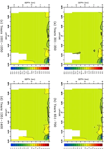
Figure 5.30: The drift in annual-meanσθ(kgm−3) during coupled model runs
5.4. THE IMPACT OF THE SPIN-UP PROCEDURE 193
(not shown). However, both runs also experience a decrease in the temperature of Antarctic Intermediate Water; this is particularly pronounced in the case of run CON-EFF, and can be attributed to the surface cooling in the Southern Ocean.
The drift in the mean salinity of the ocean is small, as with run CON-DEF. A vertical redistribution of salt is again encountered, with freshening of the surface layers and an increase in the salinity of the deep ocean. Changes in the potential density of the ocean are also small for both runs. The surface layers become slightly more buoyant, as a result of the freshening of the upper ocean; otherwise, there is a small increase in density throughout the water column.
Circulation
Figure 5.31 shows the evolution in the rates of North Atlantic Deep Water (NADW) formation and Antarctic Bottom Water (AABW) formation, and in the rate of volume transport through Drake Passage, during runs CON-SHF and CON-EFF. After some initial adjustment, the rates of deep water formation are stable for both runs. As with run CON-DEF, both runs exhibit a slight upward trend in the strength of the Antarctic Circumpolar Current.
Mean sea level
Figure 5.32 shows the changes in mean sea level inferred from runs CON-SHF and CON-EFF. As a result of the greater cooling of the world ocean, the declines in the mean sea level are greater than for run CON-DEF.
5.4.3 Climate variability
Interannual variability
Figure 5.33 shows the standard deviations in the annual-mean surface air tempera-ture (SAT) and sea surface temperatempera-ture (SST), for years 101–1100 of coupled model runs CON-SHF and CON-EFF. As with run CON-DEF, the first 100 years of each run have been excluded, in order to allow for any initial adjustment, and a high-pass filter has been applied to remove variability on timescales longer than 100 years. For both runs, the interannual variability in SAT and SST is very similar to run CON-DEF, with the only large-scale difference being that run CON-EFF exhibits greater variability over the Southern Ocean; this is the region where the largest changes were made to the amplitude of the annual cycle in the prescribed sea surface temperatures (Section 4.4).
The area-weighted global-mean standard deviations in the annual-mean SAT are 0.45◦C and 0.47◦C for runs CON-SHF and CON-EFF respectively, compared with a value of 0.45◦C for run CON-DEF. Likewise, the global-mean standard deviations in the annual-mean SST are 0.30◦C and 0.32◦C respectively, compared with a value of 0.30◦C for run CON-DEF.
5.4. THE IMPACT OF THE SPIN-UP PROCEDURE 195
Figure 5.32: The steric changes in mean sea level diagnosed from coupled model runs CON-SHF and CON-EFF.
runs CON-SHF and CON-EFF respectively, and 10.9% and 10.0%, respectively, for the leading principal components of the annual-mean SAT. These figures are very similar to those of 22.3% and 10.6% for run CON-DEF. For both the SST and the SAT, the magnitudes and spatial structures of the principal components are also very similar to those for run CON-DEF, further indicating the similarity between the interannual variability within the three runs.
El Ni˜no-Southern Oscillation
Figure 5.35 shows the correlation between the simulated SST anomalies at each gridpoint and the SOI, for runs CON-SHF and CON-EFF. The correlations are very similar to those for run CON-DEF; the only significant difference is that the increased interannual variability in the Southern Ocean sea surface temperatures within run CON-EFF tends to weaken the correlations with the SOI.
Statistics for the simulated El Ni˜no-Southern Oscillation are shown in Table 5.5. The greater internal variability within run CON-EFF gives rise to greater SST variability in the Ni˜no 3.4 region, but there are no statistically significant differences between the El Ni˜no statistics for the three runs.
5.4. THE IMPACT OF THE SPIN-UP PROCEDURE 197
5.4. THE IMPACT OF THE SPIN-UP PROCEDURE 199
CON-DEF CON-SHF CON-EFF
Correlation between Ni˜no 3.4 -0.78 -0.79 -0.77
SST anomaly and SOI
Standard deviation of Ni˜no 0.49 0.50 0.54
3.4 SST anomaly (◦C)
Average return period of El 7.8±0.5 7.4±0.5 7.2±0.5
Ni˜no events (years)
Average duration of El Ni˜no 17.5±0.9 17.2±1.0 18.3±1.0
events (months)
Average magnitude of El 0.88±0.02 0.89±0.02 0.94±0.03
Ni˜no events (◦C)
Table 5.5: Some El Ni˜no statistics for years 101–1100 of coupled model runs CON-DEF, CON-SHF and CON-EFF: the correlation between the Ni˜no 3.4 sea surface temperature (SST) anomaly and the Southern Oscillation Index (SOI); the standard deviation of the five-month running mean of the Ni˜no 3.4 SST anomaly; the average return period of El Ni˜no events; the average duration of El Ni˜no events; and the average magnitude of El Ni˜no events.
at ∼0.15 years−1
; these frequencies correpond to periods of ∼27 and ∼6.7 years respectively. Thus, as with run CON-DEF, the simulated ENSO is too weak relative to the simulated interdecadal variability in the Pacific Ocean.
The power spectrum for run CON-EFF differs, however, with more power on interannual timescales, and less on interdecadal timescales. While maximum power occurs at ∼0.025 years−1
(∼40 years), a strong secondary peak is also apparent at ∼0.12 years−1 (∼8.1 years). Although the simulated ENSO therefore remains too weak, the bias toward interdecadal variability is sharply reduced.
5.4.4 Summary
Runs CON-SHF and CON-EFF both exhibit a high degree of stability, although the global-mean surface air temperature declines slightly more rapidly than in run CON-DEF. There is an apparent correlation between the rate of drift and the mag-nitude of the flux adjustments: the heat flux adjustments employed within both runs are smaller than those employed within run CON-DEF and, in both cases, the sea surface temperature exhibits greater drift. The salinity tendency adjustments employed within run CON-SHF are also smaller than those employed within run CON-DEF, and the sea surface salinities exhibit greater drift; however, the salinity tendency adjustments employed within run CON-EFF are larger than those em-ployed within run CON-DEF, and the sea surface salinities exhibit less drift. This correlation is worthy of further investigation.
Figure 5.36: The normalised power spectra of the Ni˜no 3.4 sea surface temperature anomaly for years 101–1100 of coupled model runs CON-DEF (black), CON-SHF (red) and CON-EFF (green). Each spectrum has been smoothed through the ap-plication of a Hann window of width 25.