Hyperspectral proximal sensing of the botanical composition and nutrient content of New Zealand pastures : a thesis presented in partial fulfilment of the requirements for the degree of Doctor of Philosophy in Earth Science

Full text

(1)Copyright is owned by the Author of the thesis. Permission is given for a copy to be downloaded by an individual for the purpose of research and private study only. The thesis may not be reproduced elsewhere without the permission of the Author..

(2) Hyperspectral Proximal Sensing of the Botanical Composition and Nutrient Content of New Zealand Pastures A thesis presented in partial fulfilment of the requirements for the degree of. Doctor of Philosophy in Earth Science. at Massey University, Palmerston North, New Zealand. Ieda Del’Arco Sanches 2009.

(3)

(4) i. Abstract The potential of hyperspectral proximal sensing to quantify sward characteristics important in making critical decisions on the management of sheep and dairy pastures in New Zealand has been investigated. Hyperspectral data were acquired using an ASD FieldSpec ®. Pro FR. spectroradiometer attached to the Canopy Pasture Probe (CAPP). The CAPP was developed to enable the collection of in situ reflectance data from New Zealand pasture canopies independent of ambient light conditions. A matt white ceramic tile was selected as a reflectance standard to be used with the CAPP, after testing a variety of materials. Pasture reflectance factor spectra between 350-2500 nm (with spectral resolutions of 3 nm between 350-1000 nm and 10 nm between 1000-2500 nm) and pasture samples were collected from six hill country and lowland areas, across all seasons (August 2006 to September 2007) in a number of regions in the North Island of New Zealand. After pre-processing (e.g. spectral averaging, de-stepping, elimination of noisy wavelengths, smoothing) the spectral data collected from sites were correlated against pasture botanical composition (expressed as proportions of grass, legume and weed) and pasture nutrients (nitrogen, phosphorus, potassium, calcium, magnesium, sodium and sulphur) expressed in percentage of dry matter (%) and amount (kg ha-1) using partial least squares regressions (PLSR). The accuracy and precision of the calibrations were tested using either the full cross-validation leave-one-out method or testing datasets. Regressions were carried out using the reflectance factor data per se and after mathematical transformation, including first derivative, absorbance and continuum-removed spectra. Overall best results were obtained using the first derivative data. The quality of predictions varied greatly with the pasture attribute, site and season. Some reasonable results were achieved for the prediction of pasture grass and legume proportions when analysing samples collected during autumn (grass: R2 > 0.81 and SD/RMSEP. 2.3 and legume: R2 > 0.80 and SD/RMSEP. 2.2), but predicting pasture. weed content was poor for all sites and seasons (R2 ≤ 0.44 and SD/RMSEP ≤ 1.2). The inaccurate predictions might be explained by the fact that the diversity found in the field.

(5) ii and observed in the pasture spectral data was not taken into account in the pasture botanical separation. The potential for using proximal sensing techniques to predict pasture nutrients in situ was confirmed, with the sensing of pasture N, P and K increased by the procedure of separating the data according to the season of the year. The full potential of the technology will only be realised if a substantial dataset representing all the variability found in the field is gathered. The importance of obtaining representative datasets that embrace all the biophysical factors (e.g. pasture type, canopy structure) likely to affect the relationship, when building prediction calibrations, was highlighted in this research by the variance in the predictions for the same nutrient using different datasets, and by the inconsistency in the number of common wavelengths when examining the wavelengths contributing to the relationship. The ability to use a single model to predict multiple nutrients, or indeed individual nutrients, will only come through a good understanding of the factors likely to influence any calibration function. It has been demonstrated in this research that reasonably accurate and precise pasture nutrient predictions (R2 > 0.74 and SD/RMSEP. 2.0) can be. made from fresh in situ canopy measurements. This still falls short of the quality of the predictions reported for near infrared reflectance spectroscopy (NIRS) for dried, ground samples analysed under controlled laboratory conditions..

(6) iii. Acknowledgements I would like to show my gratitude to the Brazilian government who provided me with a CAPES scholarship (CAPES - Coordenação de Aperfeiçoamento de Pessoal de Nível Superior). I would like to sincerely thank my supervisor Mike Tuohy for his guidance and effort during my PhD and most of all for being such a wonderful friend in both academic and non-academic matters. My thanks to my co-supervisors Mike Hedley and Alec Mackay, I really appreciated all the effort you dedicated to my research, my thesis would not be the same without your ideas and comments. Thanks to Roger Parfitt (Landcare Research) for access to the plots and data from the biodiversity study and to P21 Feeds (C10X0604) for access to the plots and data from the N x P x Irrigation interaction study. To Dr P. Loganathan, Mr M. Bretherton for their trial data and Joy and Clem Smith of Alfredton for making their farm available for this study. To Martin Hawke for providing the sites at Tokoroa, Atiamuri and Manawahe. To Ian Yule, Kensuke Kawamura, Keith Betteridge and Annette Litherland, for all their assistance and exchange of experience. To all staff from Soil & Earth Sciences for their assistance throughout my study. Many thanks to all the New Zealand Centre for Precision Agriculture staff and students (and partners) for the friendship throughout my study: especially Matt (and Kathryn) and Ina. Many thanks to Bambang Kusumo for his friendship and discussions about our research. Thanks to the Brazilian community here in NZ, especially my dear friends Daniela, Luis, Ana Paula, Flavia, Matheus, Silvia and Gustavo; life in Palmerston North was much more enjoyable with you guys around. To the south-American friends I‟ve met in Palmy, specially Karin and Carlos (Hannika and Phillip), it was a pleasure to have spent this time with you. My immense gratitude to my family and friends back home for their support and encouragement. And most of all, to my husband, Francisco, I will be always glad we came to New Zealand; this time here brought us even closer. Thank you for your love, for being at my side, for being such an understanding person. And to my lovely baby daughter born in New Zealand, Sofia, life is much more colourful with you around; you bring joy and love!.

(7) iv.

(8) v. Table of Contents Abstract .............................................................................................................................. i Acknowledgements ........................................................................................................... iii Table of Contents ............................................................................................................... v List of Figures ................................................................................................................... xi List of Tables .................................................................................................................. xix List of Abbreviations .................................................................................................... xxiii CHAPTER 1: ................................................................................................................... 1 General Introduction .......................................................................................................... 1 1.1. Pastures ....................................................................................................................... 1 1.2. Remote sensing ........................................................................................................... 2 1.3. Hyperspectral proximal sensing ................................................................................... 2 1.4. Objective..................................................................................................................... 3 1.5. Outline ........................................................................................................................ 4 CHAPTER 2: ................................................................................................................... 7 A technique for acquiring in situ reflectance spectra from pastures independent of ambient conditions .......................................................................................................................... 7 Abstract ............................................................................................................................. 7 2.1. Introduction ................................................................................................................ 7 2.2. Material and methods .................................................................................................. 9 2.2.1. CAPP (canopy pasture probe) ............................................................................... 9 2.2.1.1. The frame .................................................................................................... 10 2.2.1.2. Fiber optic input position ............................................................................. 11 2.2.2. Light source ....................................................................................................... 14 2.2.3. Battery ............................................................................................................... 14 2.2.4. ASD FieldSpec Pro FR ....................................................................................... 15 2.2.5. Reflectance standard ........................................................................................... 15 2.2.6. Acquisition and pre-processing of reflectance factor spectra acquired using the Spectro-CAPP .............................................................................................................. 15.

(9) vi 2.2.7. Comparison between pasture spectra acquired with the Spectro-CAPP and with the FieldSpec® under sunlight conditions ........................................................................... 18 2.3. Results and discussion ............................................................................................... 18 2.3.1. Fiber optic input position: grip fixed on the top of the CAPP versus grip fixed on the side of the CAPP .................................................................................................... 18 2.3.2. Light source........................................................................................................ 20 2.3.3. Light and battery stability ................................................................................... 21 2.3.4. Pasture reflectance factor acquired using the CAPP ............................................ 22 2.3.5. Comparison between pasture spectra acquired with the Spectro-CAPP and with the FieldSpec® under sunlight conditions ........................................................................... 24 2.3.6. Examples of pasture swards measured using the CAPP ....................................... 25 2.4. Conclusions ............................................................................................................... 26 CHAPTER 3: ................................................................................................................. 29 Large, durable and low-cost reflectance standard for field remote sensing applications .... 29 Abstract ........................................................................................................................... 29 3.1. Introduction............................................................................................................... 29 3.2. Material and methods ................................................................................................ 32 3.2.1. Reflectance standards ......................................................................................... 32 3.2.2. Reflectance spectrometry .................................................................................... 33 3.2.2.1. FieldSpec® Pro FR attached to the ASD plant probe..................................... 34 3.2.2.2. FieldSpec® Pro FR attached to the CAPP ..................................................... 34 3.3. Results and discussion ............................................................................................... 34 3.3.1. Evaluation of a range of potential reflectance standards ...................................... 34 3.3.2. Selection of reflectance standard tile for further study......................................... 41 3.4. Conclusions ............................................................................................................... 42 CHAPTER 4: ................................................................................................................. 43 Influence of surface moisture on field hyperspectral data from pasture canopies .............. 43 Abstract ........................................................................................................................... 43 4.1. Introduction............................................................................................................... 43 4.2. Material and methods ................................................................................................ 45 4.2.1. The study area .................................................................................................... 45.

(10) vii 4.2.2. Field canopy reflectance factor measurements and chemical analysis ................. 46 4.2.3 Data pre-processing and data analysis .................................................................. 47 4.3. Results ...................................................................................................................... 48 4.3.1. Pasture samples .................................................................................................. 48 4.3.2. Reflectance factor data ....................................................................................... 49 4.3.3. T-test results ....................................................................................................... 52 4.3.4. Pasture crude protein .......................................................................................... 55 4.4. Discussion................................................................................................................. 56 4.4.1. Significant differences between treatments ......................................................... 58 4.4.2. Pasture crude protein prediction.......................................................................... 59 4.5. Conclusion ................................................................................................................ 60 CHAPTER 5: ................................................................................................................. 61 Proximal sensing the botanical composition of New Zealand dairy and sheep pastures..... 61 Abstract ........................................................................................................................... 61 5.1. Introduction .............................................................................................................. 62 5.2. Materials and methods .............................................................................................. 64 5.2.1. Study area .......................................................................................................... 64 5.2.2. Acquisition of pasture reflectance factor spectra and pasture samples ................. 65 5.2.3. Spectral data pre-processing ............................................................................... 66 5.2.4. Data analysis ...................................................................................................... 67 5.3. Results and discussion ............................................................................................... 69 5.3.1. Pasture botanical components ............................................................................. 69 5.3.2. Pasture spectra.................................................................................................... 72 5.3.3. Predictions of pasture botanical components ....................................................... 74 5.3.4. PLSR carried out separately for Colyton samples with and without added N ...... 81 5.3.5. Contrasting predictions for hill (Alfredton) and lowland (Colyton) sites ............. 82 5.3.6. Contrasting prediction for different seasons ........................................................ 83 5.4. Conclusions .............................................................................................................. 84 CHAPTER 6: ................................................................................................................. 87 Seasonal predictions of in situ pasture macro-nutrients in New Zealand pastoral systems using hyperspectral data ................................................................................................... 87.

(11) viii Abstract ........................................................................................................................... 87 6.1. Introduction............................................................................................................... 88 6.2. Material and methods ................................................................................................ 91 6.2.1. Study sites .......................................................................................................... 91 6.2.2. Field data collection............................................................................................ 92 6.2.3. Spectral data pre-processing ............................................................................... 93 6.2.4. Transformations.................................................................................................. 94 6.2.5. Regression analyses ............................................................................................ 95 6.2.5.1. Entire dataset (357 samples for N%, 473 samples for P% and 376 samples for K% prediction) ......................................................................................................... 96 6.2.5.2. Seasonal datasets ......................................................................................... 97 6.2.6. Martens‟ Uncertainty Test .................................................................................. 97 6.3. Results and discussion ............................................................................................... 98 6.3.1. Pasture chemical analysis ................................................................................... 98 6.3.2. Prediction of pasture N, P and K concentration using different mathematically transformed spectral data .............................................................................................. 99 6.3.3. Predictions of pasture nutrient concentration by season ..................................... 102 6.3.3.1. Nitrogen..................................................................................................... 103 6.3.3.2. Phosphorus ................................................................................................ 107 6.3.3.3. Potassium .................................................................................................. 110 6.3.3.4. Most important wavelengths for the pasture nutrient predictions ................ 112 6.4. Conclusions ............................................................................................................. 116 CHAPTER 7: ............................................................................................................... 119 Estimation of nutrient concentration and mass of pastures grown under different soil phosphorus status and varying nitrogen fertiliser regimes using field spectroscopy ........ 119 Abstract ......................................................................................................................... 119 7.1. Introduction............................................................................................................. 120 7.2. Materials and methods............................................................................................. 122 7.2.1. Study area......................................................................................................... 122 7.2.2. Data collection.................................................................................................. 123 7.2.3. Spectral data processing and analyses ............................................................... 123.

(12) ix 7.2.4. Chemical analyses .............................................................................................125 7.3. Results and Discussion .............................................................................................125 7.3.1. Phosphorus and Nitrogen ...................................................................................125 7.3.1.1. Effect of P and N fertilisers on grass-legume pasture composition ..............125 7.3.1.2. P and N concentration and mass ..................................................................128 7.3.1.3. Pasture reflectance factor spectra ................................................................129 7.3.1.4. Correlation between first derivative reflectance (FDR) and pasture P and N concentration and mass ...........................................................................................132 7.3.1.5. Partial least squares regression (PLSR) to predict pasture P and N concentration and mass ...........................................................................................133 7.3.2. Pasture potassium, calcium, magnesium, sodium and sulphur predictions ..........139 7.3.2.1. Pasture nutrient concentration and mass ......................................................139 7.3.2.2. Correlation with FDR .................................................................................141 7.3.2.3. Prediction of pasture K, Ca, Mg, Na and S concentration and mass using PLSR models ..........................................................................................................143 7.4. Conclusions .............................................................................................................145 CHAPTER 8: ................................................................................................................147 Prediction of the nutrient concentration and mass of hill pasture using proximal sensed hyperspectral reflectance factor .......................................................................................147 Abstract ..........................................................................................................................147 8.1. Introduction .............................................................................................................148 8.2. Materials and methods .............................................................................................149 8.2.1. Study area .........................................................................................................149 8.2.2. Data collection ..................................................................................................150 8.2.3. Spectral data processing and statistical analysis .................................................151 8.2.4. Nitrogen, phosphorus and potassium chemical analyses.....................................152 8.3. Results and Discussion .............................................................................................153 8.3.1. Pasture spectra...................................................................................................153 8.3.2. Pasture nutrient concentration and mass ............................................................155 8.3.3. Correlation between FDR and pasture nutrients .................................................156 8.3.4. Prediction of pasture nutrients ...........................................................................157.

(13) x 8.3.5. Important wavelengths...................................................................................... 161 8.4. Conclusions ............................................................................................................. 165 CHAPTER 9: ............................................................................................................... 167 Summary, general discussion, final considerations and future work recommendations ... 167 9.1. Summary, general discussion and final considerations ............................................. 167 9.1.1. Chapters 2, 3 and 4 ........................................................................................... 167 9.1.2 Chapters 5, 6, 7 and 8 ........................................................................................ 168 9.2 Future work recommendations ................................................................................. 174 REFERENCES............................................................................................................. 177.

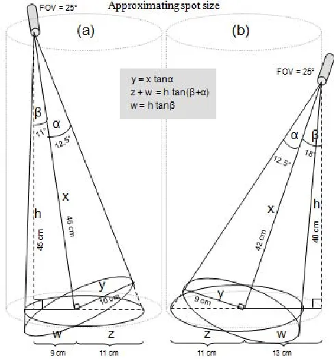
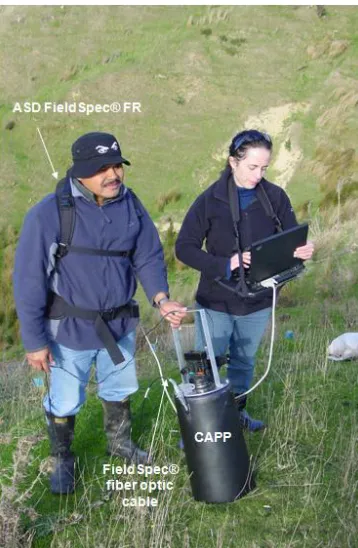
(14) xi. List of Figures. Figure 2.1. (a) CAPP with the spectroradiometer ASD FieldSpec® Pro FR; (b) ASD light source mounted on the top and fibre optic cable grips on the top and side of the CAPP; (c) acquiring reflectance spectra from sheep-grazed pasture. ................................ 10 Figure 2.2. Diagram of pasture specular and diffuse reflection being captured by the CAPP with the ASD FieldSpec® Pro FR fibre optic input placed: a) on the top of the CAPP, b) on the side of the CAPP. .................................................................................. 12 Figure 2.3. Calculating area measured within the FOV of the sensor for measurements acquired by the CAPP with the ASD FieldSpec® Pro FR fibre optic input placed: a) on the top of the CAPP, b) on the side of the CAPP. ............................................................. 12 Figure 2.4. The area inside the white circles illustrates the approximate area measured by the Specto-CAPP using the fibre optic input placed on the top of the probe and on the side of the probe, for different pasture sward heights (PSH). ...................................... 13 Figure 2.5. Spectra of a pasture measured with the Spectro-CAPP, using the fibre optic input placed on the top of the probe (continuous lines) and on the side of the probe (dashed lines), between a) 400 nm to 2500 nm, and enlarged for the spectral range between: b) 950 nm and 1050 nm; c) 1750 nm and 1850 nm. ........................................... 19 Figure 2.6. (a) Radiance (W m-2sr-1 nm-1) reflected from a reference sample (matt white ceramic tile) illuminated by the ASD 50 W Pro-lamp mounted on the CAPP. The 16 curves plotted correspond to the radiance of the reference sample when the reference panel was elevated to different heights (every centimetre between 0 to 15 cm) inside the CAPP: the curve with the lowest radiance corresponds to the reference sample placed on the ground (0 cm height), the curve with the highest radiance corresponds to the reference sample lifted 15 cm. (b) Percentage of the increase in radiance observed in the plot (a). ............................................................................................................................ 20.

(15) xii Figure 2.7. Average percentage decrease, over time, in radiance reflected from a reference sample (matt white ceramic tile) illuminated by the ASD 50 W Pro-lamp mounted on the CAPP powered by 12 v battery. The curves correspond to the decrease in radiance recorded per minute over a period of 60 minutes of battery usage (the count of the 60 minutes started after 15 min of warm up time). .................................................. 22 Figure 2.8. Spectra of pasture plots measured with the Spectro-CAPP using the fibre optic input placed on the top of the probe (continuous lines) and on the side of the probe (dashed lines), between 400-2500 nm and enlarged for the spectral ranges 950-1050 nm and 1750-1850 nm. a) Original data, b) smoothed data, c) de-stepped data and d) destepped and smoothed data. .............................................................................................. 23 Figure 2.9. Reflectance spectra (relative reflectance converted into absolute reflectance) of different pasture plots (A, B, C and D) acquired in four distinct ways: 1) matt white ceramic tile as white reference and the Spectro-CAPP top-grip (black lines), 2) ceramic tile and the Spectro-CAPP side-grip (dashed black lines), 3) ceramic tile and the FieldSpec® under sunlight (dotted grey lines), and 4) spectralon® disc as white reference and the FieldSpec® under sunlight (thick grey lines). ....................................... 25 Figure 2.10. Examples of pre-processed (de-stepped and smoothed) reflectance factor spectra of pasture swards measured with the Spectro-CAPP using the fibre optic input placed on the top of the CAPP. Sites 1 and 2 correspond to a sheep pasture on a hill country site and a dairy pasture in a flat area, respectively. The pictures of each site show how the same pasture plot appears in different seasons of the year. ......................... 26 Figure 3.1. ASD plant-probe and CAPP (canopy pasture probe). ...................................... 33 Figure 3.2. Reflectance of the materials inferred using an ASD FieldSpec ® Pro FR with an ASD plant probe using a SRT-99-050 reflectance standard: a) spectralon® (1), barium sulphates (2 and 3) and all white ceramic tiles (5, 6, 8, 9, 10 and 11); b) white paint (4), grey ceramic tile (7), grey and white cards (12, 13). .......................................... 35.

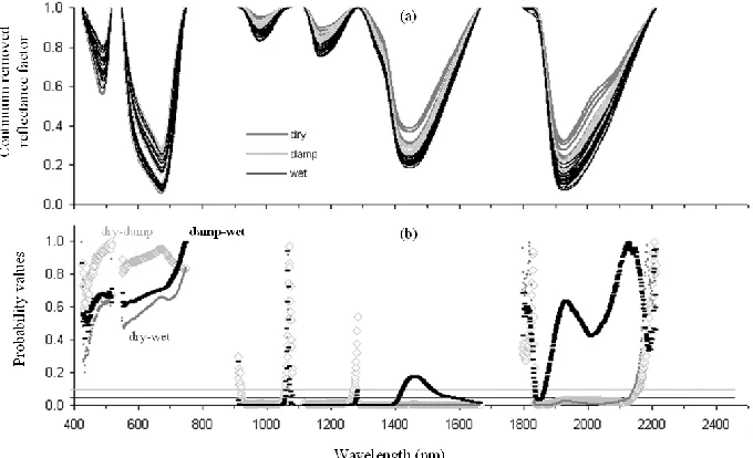
(16) xiii Figure 3.3. Spectra of a fresh green leaf obtained using an ASD FieldSpec ® Pro FR with an ASD plant probe using as reflectance standard: a) spectralon® (1), barium sulphates (2, 3), white ceramic tiles Tau Ceramica (8), Milenio Blanco (9), San Lorenzo (10), Nordico Snow (11); b) white ceramic tiles Asia Tile (5) and Niro Whites (6). .................. 37 Figure 3.4. Offset by 10% of the white reference scans of spectralon® (1), barium sulphates (2, 3), white ceramic tiles Tau Ceramica (8), Milenio Blanco (9), San Lorenzo (10) and Nordico Snow (11) taken using an ASD FieldSpec® Pro FR with an ASD plant probe................................................................................................................................ 38 Figure 3.5. Spectra of a grass canopy acquired by an ASD FieldSpec ® Pro FR with the CAPP, using the May & Baker barium sulphate (2), white ceramic tiles Tau Ceramica (8), Milenio Blanco (9), San Lorenzo (10) and Nordico Snow (11) as reflectance standards, between a) 400 nm to 2400 nm, and enlarged in the spectral range between: b) 800 nm and 1200 nm; c) 1600 nm and 2000 nm. .......................................................... 39 Figure 4.1. Collection of canopy pasture spectral data using the CAPP coupled to an ASD FieldSpec® Pro FR. ................................................................................................. 46 Figure 4.2. Photographs of pasture plots. .......................................................................... 49 Figure 4.3. Response of pasture canopy reflectance factor to the treatments dry (dark grey line), damp (light grey line) and wet (black line) for pasture plot 3 (a) and plot 7 (b). Overall hardly any change was observed at Vis; at NIR two reactions were noticed: (a) both increase and decrease in reflectance factor values, and (b) decrease in reflectance factor values at all NIR; at all MIR wavelengths the reflectance factor decreased. ............ 50 Figure 4.4. Percentage of reflectance factor difference for all samples (a) under damp treatment and (b) under wet treatment; and samples divided into two groups (c) average of 1st group under damp and wet treatment; (d) average of 2nd group under damp and wet treatment. The reflectance factor difference was calculated by subtracting the dry reflectance factor of a pasture sample from the damp reflectance factor of the same pasture and from the wet reflectance factor of the same sample. ....................................... 51.

(17) xiv Figure 4.5. Reflectance factor sensitivity to surface moisture for all (a) damp data, (b) dew data, and (c) averaged data in a zoon in scale. The reflectance factor sensitivity was calculated by dividing the reflectance factor difference by the dry reflectance factor of each sample, for damp (grey line) and wet (black line) data. ............................................. 52 Figure 4.6. (a) Reflectance factor spectra for the 20 plots analysed. And (b) results of ttest for the reflectance factor data. Three classes were considered: dry versus damp, damp versus wet, and dry versus wet. The dots plotted show the probability value when testing if the reflectance factors between classes are significantly different. Horizontal line in black and grey show 95% (p < 0.05) and 90% (p < 0.10) confidence limits correspondingly. .............................................................................................................. 53 Figure 4.7. (a) First derivative spectra averaged per treatment. And (b) results of t-test for the first derivative data of 20 plots. Three classes were considered: dry versus damp, damp versus wet, and dry versus wet. The dots plotted show the probability value when testing if the reflectance factors between classes are significantly different. Horizontal line in black and grey show 95% (p < 0.05) and 90% (p < 0.10) confidence limits correspondingly. .............................................................................................................. 54 Figure 4.8. (a) Continuum removed reflectance factor spectra for the 20 plots analysed. And (b) results of t-test for the continuum removed data. Three classes were considered: dry versus damp, damp versus wet, and dry versus wet. The dots plotted show the probability value when testing if the reflectance factors between classes are significantly different. Horizontal line in black and grey show 95% (p < 0.05) and 90% (p < 0.10) confidence limits correspondingly. ................................................................................... 55 Figure 5.1. Sampling site locations: 1) Manawahe, 2) Tokoroa, 3) Atiamuri, 4) Colyton and 5) Alfredton. .............................................................................................................. 64 Figure 5.2. Botanical proportions (grass, legume and weed) averaged per date of data collection for Alfredton and Colyton sites. ....................................................................... 71.

(18) xv Figure 5.3. Reflectance factor spectra of pasture swards collected in different seasons and sites and photographs illustrating some of the plots measured: a) spectra collected during early spring at Alfredton and Colyton; b) spectra collected at Alfredton during winter and summer. .......................................................................................................... 72 Figure 5.4. PCA score plots for entire FDR dataset (n = 404): a) plotted per site and b) plotted per season. PCA score plots for c) Alfredton samples (n = 171) and d) Colyton samples (n = 160) plotted per season. ............................................................................... 73 Figure 5.5. Relationships between measured grass percentage (x-axis) and those predicted from the PLSR full cross-validation (y-axis). .................................................... 77 Figure 5.6. Relationships between measured legume percentage (x-axis) and those predicted from the PLSR full cross-validation (y-axis). .................................................... 79 Figure 5.7. Relationships between measured weed percentage (x-axis) and those predicted from the PLSR full cross-validation (y-axis). .................................................... 81 Figure 6.1. Sampling site locations: 1) Hamilton – Ruakura, 2) Tokoroa, 3) Atiamuri, 4) Manawahe, 5) Colyton, 6) Woodville – Ballantrae, and 7) Alfredton. .............................. 91 Figure 6.2. Relationships between measured pasture nitrogen concentrations and those predicted from the FDLog(1/R) dataset for the four seasons of the year. ........................ 104 Figure 6.3. Relationships between measured pasture phosphorus concentrations and those predicted from the FDR dataset for the four seasons of the year. ........................... 108 Figure 6.4. Relationships between measured pasture potassium concentrations and those predicted from the FDR dataset for the four seasons of the year. .................................... 111 Figure 6.5. Regression coefficients of PLSR models for pasture N% prediction using the FDLog(1/R) dataset by season. Plotted in black are the significant wavelengths for the regression according to the Martens‟ Uncertainty Test. Values plotted in the graphs represent the significant wavelengths with highest regression coefficient values. ........... 113.

(19) xvi Figure 6.6. Regression coefficients of PLSR models for pasture P% prediction using the FDR dataset per season. Plotted in black are the significant wavelengths for the regression according to the Martens‟ Uncertainty Test. Values plotted in the graphs represent the significant wavelengths with highest regression coefficient values............. 115 Figure 6.7. Regression coefficients of PLSR models for pasture K% prediction using the FDR dataset per season. Plotted in black are the significant wavelengths for the regression according to the Martens‟ Uncertainty Test. Values plotted in the graphs represent the significant wavelengths with highest regression coefficient values............. 116 Figure 7.1. Photographs illustrating the legume composition of pastures receiving added P and added P+N (200kgN/ha). Averaged legume production (considering 4 cuts), which was calculated by multiplying the average legume % by the pasture mass, per treatment. ....................................................................................................................... 127 Figure 7.2. (a) Averaged reflectance factor spectra of added P and added P+N samples. (b) Percentage difference in reflectance factor, which corresponds to the percentage by which the reflectance factor of the added P averaged spectrum is higher than the added P+N averaged spectrum, at each wavelength. ................................................................. 130 Figure 7.3. Correlation between FDR and pasture N and P concentration (%) and mass (kg ha-1) for the added P (black lines) and added P+N (grey lines) samples. Wavelengths with high correlation coefficients are identified. ........................................ 133 Figure 7.4. Relationship between measured pasture P concentration (%) and mass (kg ha-1) and those predicted using PLSR cross-validation and FDR, of added P and added P+N samples separately (each with n = 80) and combined (n = 160). ............................. 134 Figure 7.5. Relationship between measured pasture N concentration (%) and mass (kg ha-1) and those predicted using PLSR cross-validation and FDR, of added P and added P+N samples separately (each with n = 80) and combined (n = 160). ............................. 135 Figure 7.6. Regression coefficients of PLSR models between FDR and pasture P concentration (%) and mass (kg ha-1) using the added P and added P+N samples.

(20) xvii analysed separately. Plotted in black are the significant wavelengths for the regression according to the Martens‟ Uncertainty Test. ................................................................... 138 Figure 7.7. Regression coefficients of PLSR models between FDR and pasture N concentration (%) and mass (kg ha-1) using the added P and added P+N samples analysed separately. Plotted in black are the significant wavelengths for the regression according to the Martens‟ Uncertainty Test. ................................................................... 139 Figure 7.8. Correlation between FDR and pasture K, Ca, Mg, Na and S concentration (%) and mass (kg ha-1) for the added P (black lines) and added P+N (grey lines) samples. ......................................................................................................................... 142 Figure 8.1. (a) Averaged reflectance factor spectra for each aspect (N – north, S – south, E – east). And (b) results of t-test considering three aspects: N versus S, N versus E and E versus S. The dots plotted show the probability value, for each wavelength, when testing if the average reflectance factor spectra between classes are significantly different. Horizontal line in dashed black shows 95% (p < 0.05) confidence limit. ......... 154 Figure 8.2. Correlation between FDR and pasture nitrogen, phosphorus and potassium concentration (%) and mass (kg ha-1) represented in the plots in black lines and grey lines, respectively. Highest correlated wavelengths are identified. .................................. 157 Figure 8.3. Relationship between measured and predicted pasture nitrogen, phosphorus and potassium concentration (%) and mass (kg ha-1) using PLSR cross-validation method. .......................................................................................................................... 159 Figure 8.4. Regression coefficients for the PLSR calibration models using crossvalidation of the FDR against pasture nitrogen, phosphorus and potassium concentration (%) and mass (kg ha-1). Plotted in black are the significant wavelengths for the regression according to the Martens‟ Uncertainty Test. .................................................. 162.

(21) xviii.

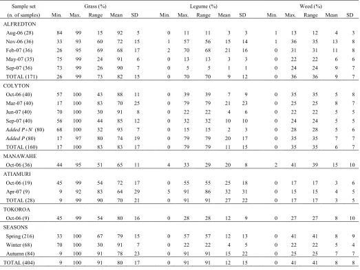
(22) xix. List of Tables. Table 2.1. Averaged change in radiance (%) at 600 nm, 1100 nm, 1600 nm and 2100 nm, over 30 minutes and 60 minutes of battery usage.............................................................. 21 Table 4.1. Wavelength intervals where the differences between wetness treatments were statistically significant (t-test) in the continuum removed spectra. .................................... 54 Table 4.2. Correlation and root mean square errors of cross-validation (RMSECV) of PLSR carried out between measured crude protein and reflectance factor, first derivative and continuum removed spectra, at Vis-IR, Vis and IR wavelength ranges, for dry, damp and wet samples. For reflectance factor and first derivative data the Vis correspond to wavelengths between 400-700 nm and IR to 700-2468 nm; for continuum removed spectra the Vis correspond to absorption bands between 425-518 nm and 550750 nm, and IR to 910-1081 nm, 1116-1284 nm, 1285-1666 nm and 1796-2214 nm. ....... 56 Table 5.1. Number of pasture samples acquired per site and corresponding date of collection. ........................................................................................................................ 65 Table 5.2. Basic statistics: minimum (Min.), maximum (Max.), range, mean and standard deviation (SD) for grass, legume and weed percentages (in fresh weight basis) in each dataset analysed. .................................................................................................. 70 Table 5.3. Statistical summary of partial least squares regression (PLSR) models fitted to predict grass percentage in different datasets. ............................................................... 76 Table 5.4. Statistical summary of partial least squares regression (PLSR) models fitted to predict legume percentage in different datasets. ........................................................... 78 Table 5.5. Statistical summary of partial least squares regression (PLSR) models fitted to predict weed percentage in different datasets. ............................................................... 80.

(23) xx Table 6.1. Number of pasture samples collected per site and per season which were analysed for N (n = 357), P (n = 474) and K (n = 377) concentration. ............................... 93 Table 6.2. Summary of statistics for pasture N, P and K concentration for entire dataset and for data divided into calibration and validation sets. ................................................... 98 Table 6.3. PLSR results between pasture nutrient concentration and reflectance factor (R), first derivative reflectance (FDR), absorbance (Log(1/R), first derivative of absorbance (FDLog(1/R)), continuum removed reflectance (CR), continuum removed derivative reflectance (CRDR), band depth ratio (BDR) and normalized band depth index (NBDI) for the validation datasets using regression models developed from the calibration datasets. ........................................................................................................ 100 Table 6.4. Summary of statistics for pasture N concentration (%) per season. ................. 103 Table 6.5. Seasonal summary of prediction statistics (PLSR full cross-validation) for pasture N% using R, FDR, and Log(1/R) data between 420-2400 nm. ............................ 104 Table 6.6. Summary of statistics for pasture P concentration (%) per season. ................. 107 Table 6.7. Seasonal summary of prediction statistics (PLSR full cross-validation) for pasture P% using R, FDR, and Log(1/R) data between 420-2400 nm. ............................ 108 Table 6.8. Summary of statistics for pasture K concentration (%) per season. ................. 110 Table 6.9. Seasonal summary of prediction statistics (PLSR full cross-validation) for pasture K% using R, FDR, and Log(1/R) data between 420-2400 nm. ............................ 111 Table 7.1. Pasture botanical composition (percentages of grass, legume and weed) for each treatment. ............................................................................................................... 126 Table 7.2. Pasture dry matter yield (kg ha -1) for each treatment considering four cuts. .... 127 Table 7.3. Summary statistics of N and P concentration (%) and mass (kg ha-1) for added P and added P+N samples separately and combined. ........................................... 128.

(24) xxi Table 7.4. Summary of PLSR (cross-validation) results for predicting N and P concentration (%) and mass (kg ha-1) of added P and added P+N samples analysed separately (each with n = 80) and combined (n = 160). .................................................. 133 Table 7.5. Summary of statistics of K, Ca, Mg, Na and S concentration (%) and mass (kg ha-1) for added P and added P+N samples separately and combined. ....................... 140 Table 7.6. Intercorrelation of measured nutrient concentration and mass, for added P and added P+N samples................................................................................................. 141 Table 7.7. Summary of PLSR (cross-validation) results for predicting K, Ca, Mg, Na and S concentration (%) and mass (kg ha-1) of added P and added P+N samples analysed separately (each with n = 80) and combined (n = 160). ................................... 144 Table 8.1. Basic statistics of pasture DM yield (kg ha-1) by aspect. DM yield values based on four cuts (August-2006, November-2006, February-2007 and May-2007). ...... 155 Table 8.2. Basic statistics of nitrogen, phosphorus and potassium concentration (%) and mass (kg ha-1) of the pasture samples analysed. .............................................................. 155 Table 8.3. Summary of results for the PLSR models developed using the FDR data to predict pasture nitrogen, phosphorus and potassium concentrations (%) and mass (kg ha1. ). Model accuracy was tested internally using leave one out cross-validation. Results. are presented for the analysis using all wavelengths between 420-2400 nm (1981 wavelengths) and when analysis was limited to the wavelengths selected by the Martens‟ Uncertainty Test. ............................................................................................. 158 Table 9.1. Comparison of the best predictions for pasture N, P and K concentration and mass (see Chapters 6 to 8). Predictions with reasonable accuracy (R2 > 0.74 and SD/RMSEP. 2.0) are highlighted (in bold). .................................................................. 173.

(25) xxii.

(26) xxiii. List of Abbreviations A. autumn. Alf.. Alfredton. ASD. Analytical Spectral Devices – ASD Inc.. Ati.. Atiamuri. Bal.. Ballantrae. CAPP. canopy pasture probe. c.f.. compare or consult. Col.. Colyton. Conc.. Concentration (%). CV. coefficient of variation. DM. dry matter. FDR. first derivative reflectance. FIA. flow injection analysis. FR. full range. ICP-OES. inductively coupled plasma-optical emission spectroscopy. IR. infrared. LV. latent variable. Max.. maximum. Man.. Manawahe. Min.. minimum. MIR. mid infrared. NIR. near infrared. NIRS. near infrared reflectance spectroscopy. PCA. principal component analysis. PLSR. partial least squares regression. PTFE. polytetrafluoroethylene. RMSE. root mean square error. RMSECV. root mean square error of cross-validation. RMSEP. root mean square error of prediction.

(27) xxiv RPD. ratio prediction to deviation. Rua.. Ruakura. SD. standard deviation. Sp. spring. Su. summer. SWIR. short-wave infrared. Tok.. Tokoroa. Vis. visible. W. winter.

(28) 1. Chapter 1. CHAPTER 1: General Introduction 1.1. Pastures The grazing lands of the world are a major source of animal feed. Although the use of crops as livestock supplementation is growing, with the increasing emphasis on sustainable farming, pasture systems remain important, needing to be managed efficiently to sustain profitability (Riveros 1993). In New Zealand, legume-based pastures grazed in situ are the main source of feed for livestock (mainly the ruminants sheep, beef, dairy, deer and goats). Pasture is grazed all year round as a consequence of the warm and moist climate, which promotes pasture growth and enables ruminants to graze outdoors throughout the year (Guy 1993, Neeley and Parminter 1993). New Zealand‟s grasslands vary in composition, distribution and productivity according to changes in landform, climate, soil and nutrient and livestock management. Overall the soils are naturally acid with moderate to low chemical fertility, and current pasture production is based on genetically improved plants topdressed regularly with lime, and phosphate, sulfur and potassic fertilizers (Daly 1990). Pasture quality is a key determinant of animal productivity and farm profitability. Pasture quality is influenced by several management factors but principally vigorous clover and ryegrass growth driven by soil fertility and grazing management (White and Hodgson 1999). Managing high pasture quality through fertilizer inputs and pasture renovation incur the largest expenditure on most farms. Apart from a method for visual estimation of quality (Meat New Zealand 2009), farmers have no large scale objective management tool at hand to assist decisions on pasture quality management. Recently published literature (Dymond et al. 2006) suggest that near infrared reflectance spectroscopy, already used to assess the quality of dried forages in the laboratory (Roberts et al. 2004), could be applied in the field to supply farmers with “in the paddock” read out of pasture quality. Such information could be used directly to improve the efficiency of nutrient use via targeted fertilizer application or grazing management..

(29) Chapter 1. 2. 1.2. Remote sensing There are several definitions of remote sensing, such as “remote sensing is the science or art of obtaining information about an object, area or phenomenon through the analysis of data acquired by a device that is not in contact with the object, area or phenomenon under investigation” (Lillesand et al. 2007); and “remote sensing consists of the interpretation of measurements of electromagnetic energy reflected from or emitted by a target from a vantage-point that is distant from the target” (Mather 1999). All definitions share the same central concept, that remote sensing is the gathering of information at a distance (Campbell 2007), and that distance defines the levels of remote sensing data collection, given that in order for a sensor to collect and record the electromagnetic energy reflected or emitted from a target on the Earth‟s surface, it needs to be placed on a platform away from the surface being observed, and the platform can be based on the ground (laboratory or field), on an aircraft (airborne) or on a satellite (spaceborne) (Cracknell and Hayes 2007). To distinguish field remote sensing, from airborne or satellite, it has recently been referred to as proximal sensing. 1.3. Hyperspectral proximal sensing In this thesis, hyperspectral proximal sensing (field remote sensing) is used to study the quality and quantity of pasture swards. Traditional multispectral remote sensing involves examination of features observed in several broad regions of the electromagnetic spectrum. Hyperspectral remote sensing examines many, very narrow contiguous spectral bands. Since hyperspectral data have more detail and greater accuracy it permits the observation of characteristics of vegetated surfaces (such as foliar chemistry) not feasible with multispectral data (Campbell 2007). Forty-two absorption features in visible and nearinfrared wavebands have been related to particular foliar chemical concentrations (cellulose, chlorophyll a and b, lignin, nitrogen, oil, protein, starch, sugar and water), showing the relationship between plant chemical constituents and the absorption of electromagnetic radiation (Curran 1989). Remote sensing of plant biochemical constituents is complex, due.

(30) Chapter 1. 3. to reflectance from vegetation being strongly influenced by the optical properties of plant materials. Different plant materials, like proteins, lignin, cellulose, etc, have similar absorptions, and a single absorption band can not be directly related to the chemical abundance of one single plant component (Kokaly and Clark 1999). The information on vegetation that can be extracted from remote sensing data depends on the capabilities of sensors, the knowledge about the interaction between radiation and vegetation canopy, and methodology used (Curran 1989). Remote sensing techniques have proved to be useful for assessing the concentration of foliar biochemicals under controlled laboratory conditions. More investigation is required to assess their capabilities in the field (Mutanga et al. 2004). Hyperspectral remote sensing provides the potential for a significant jump in the quality of spectral data obtained about earth surface features (Lillesand et al. 2007), and recent studies show that the narrow bands may be crucial for providing additional information with significant improvements over broad bands in quantifying biophysical characteristics of vegetation (Thenkabail et al. 2000). 1.4. Objective The objective of this study was to investigate the potential of hyperspectral proximal sensing to describe and quantify sward characteristics that are important in making critical decisions on the management of sheep and dairy pastures in New Zealand. The hypothesis is that sufficient sensitivity and consistency in the sensing of vegetated surfaces can be obtained in situ with hyperspectral proximal sensing, not possible with multispectral approaches, and such spectral data can be calibrated to pasture sward characteristics of economic importance. The resultant calibration should be robust and portable across a diversity of pasture swards. Specific objectives included: (a) develop a technique which enables the collection of in situ reflectance data from pasture canopies independent of ambient conditions; (b) evaluate the possibility of proximally sensing the botanical composition of grass-legume based pastures; and (c) explore the prediction of pasture nutrient concentration and mass of swards over contrasting soil fertility, landscapes (hill country site and lowland areas) and seasons of the year..

(31) Chapter 1. 4. 1.5. Outline The thesis consists of 9 chapters, 7 of which are written and presented as standalone research papers. Two papers have been submitted to the International Journal of Remote Sensing: one has been accepted (Chapter 3) and the other is under revision (Chapter 2). Chapter 1: General Introduction. Introduces the subject, the objective and structure of the thesis and briefly outlines each chapter. Chapter 2: A technique for acquiring in situ reflectance spectra from pastures independent of ambient conditions (A paper from this study has been submitted to the International Journal of Remote Sensing – In review). New Zealand‟s changeable weather and cloud cover represent a challenge for the timely collection of spectral data in situ under sunlight illumination. The Canopy Pasture Probe (CAPP) was developed to overcome this problem, to enable spectral data to be collected independently of ambient conditions. The Chapter describes the CAPP; how spectral measurements are obtained using the CAPP attached to an ASD FieldSpec® Pro FR spectroradiometer; provides examples of pasture swards measured using the CAPP; and shows the differences between canopy pasture spectra collected in situ using the CAPP compared to measurements under natural sunlight. Chapter 3: Large, durable and low-cost reflectance standard for field remote sensing applications (A paper from this study has been published in the International Journal of Remote Sensing). The development of the CAPP required a suitable large reflectance standard. To purchase a traditional reflectance standard panel (such as Spectralon®) large enough to be used with the CAPP (greater than 20 cm diameter) would be expensive. This Chapter describes the search for a large, durable and low cost reflectance standard. A variety of materials (ceramic tiles, barium sulphate powders, white paint and a Kodak card) are evaluated, and a matt white ceramic tile was selected..

(32) Chapter 1. 5. Chapter 4: Influence of surface moisture on field hyperspectral data from pasture canopies. The CAPP has been proven very efficient in controlling the illumination, and as a wind barrier to keep the target still during spectral measurements. Unfortunately not all atmospheric influences can be controlled under field conditions, and although the sunlight and wind are not a concern when using the CAPP, the target surface moisture can be. This Chapter examines the effect of surface moisture upon in situ hyperspectral data collected from pasture canopies. Chapter 5: Proximal sensing the botanical composition of New Zealand dairy and sheep pastures. For pastoral farming systems, information on the botanical composition of swards is important in pasture management and in determining both the quantity and quality of forage. In this Chapter, the potential of using proximal sensing to obtain information on the botanical composition (grass, legume and weed contents) of New Zealand dairy and sheep pastures is evaluated. Chapter 6: Seasonal predictions of in situ pasture macro-nutrients in New Zealand pastoral systems using hyperspectral data. In temperate regions of humid climatic regimes, the deficiency of one or more essential mineral nutrients is the most common limitation to optimum pasture growth. The ability to predict pasture nutrient content at critical times of the year is essential. This Chapter investigates the ability of proximal sensing to predict pasture macro-nutrients (nitrogen, phosphorus and potassium) in each of the four seasons of the year. Chapter 7: Estimation of nutrient concentration and mass of pastures grown under different soil phosphorus status and varying nitrogen fertiliser regimes using field spectroscopy. The ability to predict pasture nutrient content in situ may vary for swards of different characteristics. A change in nutrient unit, such as the conversion of mineral concentration (percent of dry matter) into mass (kg ha-1), might be an option to improve the proximal estimation of nutrients in forages. This Chapter explores the prediction (from reflectance factor spectra recorded in situ) of nutrient (nitrogen, phosphorus, potassium,.

(33) Chapter 1. 6. calcium, magnesium, sodium and sulphur) concentration and mass by lowland dairy pastures swards with changing soil Olsen P status and N fertiliser inputs. Chapter 8: Prediction of the nutrient concentration and mass of hill pasture using proximal sensed hyperspectral reflectance. Low soil fertility is a major factor limiting pasture production on hill country. Compared to lowland areas, hill pasture plant communities are much more complex, due to the high variability within very short distances. Slope and aspect influences livestock grazing, camping behaviour, soil fertility and the quality of the pasture. For appropriate management of hill pastures data from within paddocks are required to cover the diversity found in the field. This Chapter evaluates the prediction of mineral nutrient concentrations and masses (nitrogen, phosphorus and potassium) in hill country pasture swards on slopes > 20° and on north, east and southfacing aspects under sheep grazing, using hyperspectral proximal sensing. Chapter 9: Summarizes the findings of this project and recommends future study directions..

(34) 7. Chapter 2. CHAPTER 2: A technique for acquiring in situ reflectance spectra from pastures independent of ambient conditions -----------------------------------------------------------------------------------------------------------A paper from this study has been submitted to the International Journal of Remote Sensing: Sanches, I. D., Tuohy, M. P. and Hedley, M. J. (XXXX). A technique for acquiring in situ reflectance spectra from pastures independent of ambient illumination conditions. International Journal of Remote Sensing. XX, XXXX-XXXX. Submitted on May 2008. Revised on August 2009. Currently with referees. -----------------------------------------------------------------------------------------------------------Abstract For the collection of pasture reflectance spectra in field conditions, the CAPP (canopy pasture probe) was developed. It consists of an inverted black plastic bin with a 50 Watt tungsten-quartz-halogen light source mounted on the top and a grip to insert the fibre optic input of an ASD FieldSpec® Pro FR. The independent light source allows acquisition of consistent reflectance spectra in variable or poor natural light conditions. Spectral measurements can be taken in different seasons of the year under identical conditions of illumination and view angle, allowing the acquisition of reproducible measurements. The CAPP has been successfully used to collect reflectance factor data from New Zealand pastures, a task that can be very difficult when relying on natural illumination because rapidly changing cloud cover and weather are characteristic conditions in this country. Keywords: field spectroscopy; artificial illumination; field probe; pasture canopy. 2.1. Introduction Reflectance from vegetation surfaces is a complex phenomenon. There are several factors that influence vegetation spectral measurements, such as target reflectance.

(35) Chapter 2. 8. properties (Knipling 1970), atmospheric conditions (Kriebel 1976), solar zenith angle (Kimes 1980), sensor characteristics, clouds and winds (Curtiss and Goetz 1994). Under natural conditions, cloud-free sky, minimal atmospheric turbidity and high sun elevations are required to acquire accurate spectral data (Williams and Wood Jr. 1987). In the field, a practical and frequently utilized method to record reflectance measurements is to represent reflectance as a reflectance factor; this quantity is defined as the ratio of the radiant flux reflected by a surface to that reflected into the same reflectedbeam geometry by an ideal, perfectly diffuse, standard surface irradiated under the same conditions (Nicodemus et al. 1977). However if the illumination conditions vary between the moment the reference and target materials are measured the resultant spectra will present errors (Curtiss and Goetz 1994). New Zealand lies between latitudes 34° 04‟ S and 47° 02‟ S, and changeable weather is a common characteristic of mid-latitude areas, especially in maritime situations. Because of its oceanic position in the westerly wind belt, the atmosphere over this country is rarely still (Garnier 1958). Both the frontal systems across the ocean and the rugged landscape have a major influence on the New Zealand weather; over land and at the coast, clouds are formed through mechanical turbulence, convection and orographic ascent (Beatson 1985). An analysis of 30 localities in this country found that cloud frequency ranged from 56 to 92%. This estimation was based on daily NOAA7 satellite images over 347 days (not considering winter months), from November 1982 to April 1984 (Wardle 1986). Accordingly, the changeable weather and cloud cover present a great challenge for the successful use of passive optical proximal sensing technology in New Zealand. One option to enable more control over illumination and to acquire measurements during non-optimal conditions is to use an artificial light source. Artificial illumination has been traditionally used in laboratory spectroscopy, but the collection and transportation of the samples to a laboratory can be time-consuming, undesirable or even impossible considering the destructive characteristic of the method. To avoid the time-varying nature of the irradiance and to minimize the time spent between the collection of samples in the field and the measurement of spectral reflectance in the laboratory, Williams and Wood Jr. (1987) developed the Transportable Hemispherical Illumination System (THIS), a stable source of hemispherical illumination.

(36) Chapter 2. 9. which could be transported to the area where the study would be conducted. The idea was to bring the laboratory to the samples, instead of the samples to the laboratory. More recently a range of contact devices has been developed by ASD Inc. for the measurement of small targets (e.g. leaves), and although the size of the objects that can be measured is limited, the integral light source of these devices permits measurements to be made in the field independently of the natural illumination, and moreover, the measurements are highly reproducible (Milton et al. 2007). In our case the objective was to use a portable spectroradiometer (ASD FieldSpec® Pro FR - ASD Inc., Boulder, CO) to measure reflectance of pasture canopies in the field, using a non-destructive approach, in different seasons of the year, even under non-optimal conditions (e.g. cloud cover, wind). Since no existing device was suitable for our needs, the CAPP (canopy pasture probe) was developed. The CAPP is described in this paper, and it has been successfully used to collect reflectance factor data from dairy and sheep-grazed pastures on flat and steep topography, respectively. These data were collected to assess the feasibility of predicting pasture mineral nutrients using proximal sensing techniques. Although the idea of taking the laboratory (controlled conditions) to the field is not new, to the authors‟ knowledge there is no other hand-held device currently being used which ensures a controlled environment for the use of spectroradiometers to measure pasture canopies in situ without destroying the target. In the remaining text the term Spectro-CAPP was adopted to refer to the combined use of an ASD FieldSpec® Pro FR spectroradiometer attached to the canopy pasture probe. 2.2. Material and methods 2.2.1. CAPP (canopy pasture probe) The CAPP consists of an inverted rounded black plastic bin, painted inside with a flat black paint; it is 45 cm high and has a diameter of 26 cm (Figure 2.1). Mounted in the top is a 50 Watt ASD Pro-lamp with a tungsten-quartz-halogen bulb. The light was placed in the top centre of the instrument at zenith, and it is powered by 12 volt battery. To insert the spectroradiometer fibre optic, a grip was initially fixed on the top of the probe beside.

(37) Chapter 2. 10. the lamp, i.e. 45 cm from the target and pointing at approximately 11 degrees; later another grip was fixed on the side of the CAPP, at 40 cm height and 18 degrees from zenith. The field-of-view (FOV) of the spectroradiometer used is 25 degrees and the potential area viewed by the instrument (area measured) is very close to a circle with a diameter of approximately 20 cm. For the reflectance standard a square, matt white ceramic tile, measuring 295x295 mm was used (Sanches et al. 2009, Chapter 3).. Figure 2.1. (a) CAPP with the spectroradiometer ASD FieldSpec® Pro FR; (b) ASD light source mounted on the top and fibre optic cable grips on the top and side of the CAPP; (c) acquiring reflectance spectra from sheep-grazed pasture. 2.2.1.1. The frame The CAPP was made of a resistant plastic suitable for field work conditions. Although the plastic used was already in black colour, the interior of the bin was painted with a flat black paint to minimize any reflectance from this surface. The paint used (Dulux Quick DryTM SparykoteTM) is spectrally non selective for the range analysed (350-2500 nm) and has very low reflectance (around 0.06) (the paint‟s reflectance was measured using the ASD FieldSpec® Pro FR attached to an ASD plant probe and a spectralon® panel as.

(38) Chapter 2. 11. reflectance standard). The CAPP‟s frame is light enough to be easily carried along with the backpack-mounted spectroradiometer; and most importantly, it blocks any interference from the outside environment during the measurements, such as secondary sources of illumination and wind. 2.2.1.2. Fiber optic input position There are two types of reflectance from Earth-surface materials, specular and diffuse (Lambertian). For specular, the angle of incidence and reflection of the energy are equal and no scattering occurs at the surface. For diffuse reflectance, the radiance incident upon the surface is backscattered in all upward directions (Mather 1999). The diffuse component of reflectance from plant leaves comes mainly from inside the leaf, whereas the specular component arises primarily from the leaf surface (Grant 1987, Brakke 1994). The spectral variation of the diffuse reflection depends on leaf biochemistry and so can be used to predict the amount of leaf constituents (Bousquet et al. 2005). In most natural materials, like in vegetation targets, the diffuse reflectance is more abundant and causes fewer measurement problems (Hatchell 1999). Nevertheless, because the specular reflection depends on surface biophysical properties it can be useful for studies of refractive index and roughness of the epidermis/cuticle layer (Bousquet et al. 2005). Since the CAPP was developed to assist studies for the prediction of pasture biochemistry, our interest was to measure the diffuse reflectance and avoid the specular reflectance. One way to avoid measuring specular reflectance is to set the spectroradiometer sensor input far away from the specular plane, for example by placing the sensor input at a right angle to the illumination source (Hatchell 1999). Since this set up of right angle was not compatible with the physical structure of the CAPP, two other set ups were tested. The choice for the set ups was guided by the objective to measure a circular area of at least 15 cm diameter (considering the FOV of the spectroradiometer of 25 degrees), with a probe that was practical for field work. Two different mounting positions for the FieldSpec® Pro FR fibre optic grip on the CAPP were tested. For position 1, the grip was fixed on the top of the probe (45 cm height) at 11 degrees to the light source (Figures 2.2a and 2.3a). For position 2, the cable grip was moved from the top to the side of the probe; it was placed at 40 cm height and 18 degrees from zenith (Figures 2.2b and 2.3b). The intention was not to.

(39) Chapter 2. 12. have a probe with two different configurations, but to test if at least one of the probes would suit our needs.. Figure 2.2. Diagram of pasture specular and diffuse reflection being captured by the CAPP with the ASD FieldSpec® Pro FR fibre optic input placed: a) on the top of the CAPP, b) on the side of the CAPP.. Figure 2.3. Calculating area measured within the FOV of the sensor for measurements acquired by the CAPP with the ASD FieldSpec® Pro FR fibre optic input placed: a) on the top of the CAPP, b) on the side of the CAPP..

(40) Chapter 2. 13. The area measured by the Spectro-CAPP, as demonstrated in Figure 2.3, is slightly different for each set-up, but the potential ground area viewed by both set-ups corresponds closely to a circle with a diameter of approximately 20 cm. However, for both set ups the actual area measured will depend on the pasture sward height (PSH), since the distance between sensor input and target will decrease with any increase of the pasture height. The change in measured area by the Spectro-CAPP (top and side-grips) for a pasture sward with different heights is illustrated in Figure 2.4. One factor to be considered is that comparing two pasture plots of equal size, one with a sward higher than the other, the plot with higher sward might need more spectral measurements to be taken (measurements posterior averaged) in order to cover the same area (c.f. fig 2.4 PSH = 15 cm and PSH = 5 cm); especially for the side-grip set-up, where the area measured is slightly smaller than with the top-grip set-up.. Figure 2.4. The area inside the white circles illustrates the approximate area measured by the Specto-CAPP using the fibre optic input placed on the top of the probe and on the side of the probe, for different pasture sward heights (PSH)..

(41) Chapter 2. 14. 2.2.2. Light source There are several kinds of radiant energy generators that can be used as artificial illumination sources, such as filament and gaseous emitters excited by electrical power, burning gaseous and solid emitters, or heated gaseous and solid emitters. The most appropriate option to obtain a smooth energy output when measuring spectral data between 350 and 2500 nm is a bulb with tungsten filament emitter, a non absorbing gas (halogen) and a non absorbing envelope (quartz) (Hatchell 1999). The lamp mounted on the top of the CAPP was an ASD 50 Watt tungsten-quartzhalogen Pro-lamp (ASD Inc., Boulder, CO), which was set at maximum intensity in order to avoid noise problems. The stability of the light source was assessed. The spectral radiance of a matt white ceramic tile was measured at 1-minute intervals over 30 minutes using the Spectro-CAPP plugged in to mains power (as opposed to running on batteries). Because the lamp is fixed, the distance between the light source and the target will vary with PSH. Consequently PSH will have an effect on the irradiance (amount of flux per unit area of a defined surface) on the target, the higher the PSH the higher will be the irradiance on the target. The spectral measurement of our interest is the reflectance factor, a ratio which is independent of the irradiance. So as long as the irradiance on the reflectance standard is the same as the irradiance on the target, the measurements will be coherent despite of PSH. This subject is further discussed in the text. 2.2.3. Battery The CAPP‟s light source is powered by a 12 volt rechargeable battery. Since the overall goal for illumination is to keep it consistent, the battery stability was tested. The ideal would be to scan the reflectance standard just before each target sample is scanned to account for any variation in battery power, but because this is not always feasible when working in field conditions, it is important to know the change in radiance one can expect when dealing with a battery powered light source. The influence of variation in battery power was evaluated by using Spectro-CAPP to measure the spectral radiance of a matt.

No results found