Signal processing methods for genomic sequence analysis

(1)

Thesis by

Byung-Jun Yoon

In Partial Fulfillment of the Requirements for the Degree of

Doctor of Philosophy

California Institute of Technology Pasadena, California

2007

(2)

c

2007

(3)

Acknowledgments

First of all, I would like to express my deepest gratitude to my advisor, Professor P. P. Vaidyanathan, for his excellent guidance and support throughout my graduate studies. In fact, he was the best advisor, mentor, teacher, and researcher, I could ever think of. From my very first day at Caltech, he was always there for me whenever I needed his guidance. He taught me so many important things that are fundamental to a good researcher, for example, how to think creatively, how to develop ideas, how to write good papers, how to be a good presenter, and most importantly, how to stand alone as an independent researcher. It has been my greatest pleasure to learn from P. P., who was the perfect role model.

I also would like to thank the members of my defense and candidacy committees: Professor Yaser S. Abu-Mostafa, Professor Babak Hassibi, Professor Christina D. Smolke, Professor Tracey Ho, Professor John Doyle, Professor Changhuei Yang, and Professor Morteza Gharib. I also would like to thank the Microsoft Research, the Korea Foundation for Advanced Studies (KFAS), the Na-tional Science Foundation (NSF), and the Office of Naval Research (ONR) for their generous finan-cial support during my graduate studies at Caltech.

One of the greatest things at Caltech was the opportunity to work with some of the brightest people in the world! I truly enjoyed working with my labmates in the Digital Signal Processing (DSP) lab, and my warmest appreciation goes to them: Dr. Bojan Vrcelj, Dr. Andre Tkacenko, Sriram Murali, Borching Su, Michael Larsen, Chun-Yang Chen, and Ching-Chih Weng. Thanks to these wonderful guys, working in the DSP lab was a sheer pleasure. I will deeply miss our discussions and conversations as well as the many conference trips that we made together. I also would like to thank Andrea Boyle, our wonderful secretary, for her kind assistance and professional support.

(4)

Malvar during the first two internships and with Dr. Ivan Tashev during the third one. Rico was an extremely good mentor, who showed me what it means to maintain a perfect balance between theoretical research and practical applications. Although he was really busy with his work (well, you may not believe how many meetings he has as a director of MSR), he always found time for discussions and informal chats. I met Ivan during my third internship, where we worked on a project to develop a new adaptive microphone array processing algorithm. Ivan was a passionate mentor and he was very supportive and helpful throughout my internship. In fact, he taught me from A to Z about microphone arrays, although he himself was occupied with so many other things. During the project, I had a chance to build a linear microphone array by myself (it involved designing the array, cutting the plastic board using a laser cutter, soldering the wires, etc.), which was great fun! I am truly grateful to my MSR mentors, Rico and Ivan, who gave me these invaluable experiences that I will never forget.

I also would like to express my appreciation to my spiritual mentors, Pastor Chul-Min Kim and Pastor Byungjoo Song. I personally got to know Pastor Kim when I was a college student. At that time, I was still young and immature, and I was not so much interested in spiritual things. However, great passion is contagious, and my life started to change due to his unceasing passion for God and his constant love, care, and prayer for me. If Pastor Kim was the one who planted the seed of faith in me, it was Pastor Song who watered it so that it can grow further. Pastor Song was my mentor for the one-on-one discipleship training at the All Nations Church (a.k.a. Onnuri Church, LA). Being a passionate preacher, good theologian and apologist, he taught me many of the important Christian doctrines in a clear and logical manner. Both mentors have had a crucial impact in shaping myself as a Christian, and I hope I can live as I was taught and as I now believe. One of life’s greatest joys is to meet someone who can (and wants to) truly understand you. In this respect, I was greatly blessed to have many friends with whom I could share every aspect of my life. I am especially thankful to my Caltech friends Wonjin Jang and Hyunjoo Lee, for their friendship and support throughout my graduate studies. I can hardly imagine myself studying at Caltech without these awesome friends. My warmest thanks also goes to Chul-Gi Min and Jun-Sang Lee, my best friends in Korea, whom I have known since my (junior) high-school days.

(5)

my life, and I am really indebted to them for their sacrificial love. I am also grateful to my sister, Young-Ran Yoon, for being the best sister I could ever dream of! I also would like to thank my relatives for their encouragements and kind support. Especially, I would like to thank my uncle and aunt, Kang-Yeol Yoon and Nam-Hee Shin, and also aunt Hyo-Im Yoo for their amazing love!

Last, but by no means least, I would like to thank God, who has been always so faithful to me. As the apostle Paul has confessed, I am what I am by the amazing grace of God. Even though I did not deserve it, He never stopped loving me, and He has been (and He always will be) leading my life according to His perfect plan that is far beyond my imagination! I pray that I may glorify Him through everything I do, and enjoy Him – andonlyHim – throughout my entire life.

(6)

Abstract

Signal processing is the art of representing, transforming, analyzing, and manipulating signals. It deals with a wide range of signals, from speech and audio signals to images and video signals, and many others. Signal processing techniques have been found very useful in diverse applica-tions. Traditional applications include signal enhancement, denoising, speech recognition, audio and image compression, radar signal processing, and digital communications, just to name a few. In recent years, signal processing techniques have been also applied to the analysis of biological data with considerable success. For example, they have been used for predicting protein-coding genes, analyzing ECG signals and MRI data, enhancing and normalizing DNA microarray images, modeling gene regulatory networks, and so forth.

In this thesis, we consider the application of signal processing methods to the analysis of bio-logical sequences, especially, DNA and RNA molecules. We demonstrate how conventional signal processing techniques–such as digital filters and filter banks–can contribute to this end, and also show how we can extend the traditional models–such as the hidden Markov models (HMMs)–to better serve this purpose.

(7)

power of the model significantly, making csHMMs capable of representing long-range correlations between distant symbols. Based on the proposed model, we present efficient algorithms that can be used for finding the optimal state sequence and computing the probability of an observed symbol string. We also present a training algorithm that can be used for optimizing the parameters of a csHMM. We give several examples that illustrate how csHMMs can be used for modeling various RNA secondary structures and recognizing them.

Based on the concept of csHMM, we introduce profile-csHMMs, which are specifically con-structed csHMMs that have linear repetitive structures (i.e., state-transition diagrams). Profile-csHMMs are especially useful for building probabilistic representations of RNA sequence families, including pseudoknots. We also propose a dynamic programming algorithm called the sequential component adjoining (SCA) algorithm that can systematically find the optimal state sequence of an observed symbol string based on a profile-csHMM. In order to demonstrate the effectiveness of profile-csHMMs, we build a structural alignment tool for RNA sequences and show that the profile-csHMM approach can yield highly accurate predictions at a relatively low computational cost. At the end, we describe how the profile-csHMM can be used for finding homologous RNAs, and we propose a practical scheme for making the search significantly faster without affecting the prediction accuracy.

(8)

List of Figures

1.1 DFTs of periodic signals. (Top) Magnitude plot of the DFT of a signal with a period

T = 3. (Bottom) Magnitude plot of the DFT of a signal with a periodT = 351/117.5. . 3

1.2 The DFT of a periodic signal with a periodT = 3buried in Gaussian noise. We can observe a clear peak atk=N/3. . . 4

1.3 Example of a state transition diagram that represents a Markov chain with two distinct statesS1andS2. . . 6

1.4 Illustration of the doubly embedded stochastic process in HMMs. The stochastic pro-cess consists of an observable symbol sequence and a hidden state sequence. . . 8

1.5 Example of a state transition diagram that represents a hidden Markov model with three statesS={S1, S2, S3}and two distinct observation symbolsA={a, b}. The ini-tial state distribution and the state transition probabilities are shown along the edges and the emission probabilities are shown in the boxes. . . 8

1.6 Illustration of a nucleotide and a DNA strand. . . 12

1.7 Illustration of a DNA double helix. . . 12

1.8 Example of a DNA double helix that has been straightened out for simplicity. . . 13

1.9 The central dogma of molecular biology states that the genetic information flows from DNA to RNA to protein. . . 14

1.10 Illustration of a typical protein synthesis process. . . 15

1.11 The genetic code. . . 16

1.12 Two examples of RNAs with secondary structures. The primary sequence of each RNA is shown along with its structure after folding. The dashed lines indicate inter-actions between bases. (a) RNA with two stem-loops. (b) RNA with a pseudoknot. . . 17

(14)

2.2 Examples of sequences that are included in the palindrome language. The lines

indi-cate the pairwise correlations between distant symbols. . . 28

2.3 The statesPnandCnassociated with a stackZn. . . 30

2.4 An example of a context-sensitive HMM that generates only palindromes. . . 33

2.5 An example of a simple context-sensitive HMM. . . 35

2.6 Examples of interactions in a symbol string. The dotted lines indicate the pairwise de-pendencies between symbols. (a), (b), (c) Nested interactions. (d) Crossing interactions. 37 2.7 Examples of state sequences (a) that are considered in computingγ(i, j, v, w)and (b) those that are not considered. . . 38

2.8 Illustration of the iteration step of the algorithm. . . 42

2.9 Illustration of the iteration step of the algorithm for the case whensi=Pnandsj =Cn. 43 2.10 Examples of state sequences (a) that are considered in computingβ(i, j, v, w)and (b) those that are not considered. . . 48

2.11 Illustration of the iteration step of the outside algorithm. (a) Case (ii). (b) Case (iii). (c) Case (iv). . . 51

2.12 Illustration of the iteration step of the outside algorithm. (a) Case (v). (b) Case (vi). (c) Case (viii). . . 52

2.13 An example of a context-sensitive HMM. . . 55

2.14 The arithmetic mean (top) and the geometric mean (bottom) after each iteration. . . . 58

2.15 An example sequence that can be generated by the modified model of Figure 2.4. . . . 59

2.16 (a) A csHMM that results in crossing interactions. (b) An example of a generated symbol sequence. The lines indicate the correlations between symbols. . . 60

2.17 (a) A csHMM that represents a copy language. (b) An example of a generated symbol sequence. . . 60

2.18 An illustration of the basic concept of the algorithm that can be used when there exist crossing interactions. The dotted lines show examples of correlations that can be taken into consideration based on this setting. . . 61

(15)

3.1 Two common mechanisms of riboswitches in bacteria. (a)Translation control. In the presence of the effector metabolite, the riboswitch changes its structure and sequesters the ribosome-binding site (RBS). This inhibits the translation initiation, thereby down-regulating the gene. (b) Transcription control. Upon binding the metabolite, the ri-boswitch forms a terminator stem, which prevents the generation of the full-size mRNA. 67 3.2 An example of a profile-HMM. It repetitively uses a set of match, insert, and delete

states to model each position in a multiple sequence alignment. . . 69

3.3 Ungapped alignment between two RNA sequences. (a) An RNA with a stem-loop structure is used as the query sequence. (b) A structurally homologous RNA that has also a stem-loop structure. (c) A structurally nonhomologous RNA that does not fold to a stem-loop structure. . . 70

3.4 Compensatory mutations give rise to strong pairwise correlations in the primary se-quence of an RNA. . . 71

3.5 (a) A typical stem-loop. The nodes represent the bases in the RNA, and the dotted lines indicate the interactions between bases that form complementary base pairs. (b) An example of a csHMM that generates a sequence with a stem-loop structure. (c) A csHMM that models a stem-loop with bulges. . . 74

3.6 (a) A typical structure of an iron response element. (b) An example of a csHMM that generates sequences with the given secondary structure. . . 74

3.7 (a) A typical tRNA cloverleaf structure. (b) An example of a csHMM that can generate sequences with the cloverleaf structure. . . 75

3.8 Two different update schemes. (a) When using the variableγ(i, d, v, w). (b) When using the variableγ(j, d, v, w). . . 77

3.9 Illustration of step (v). . . 78

3.10 Illustration of step (vi). . . 79

3.11 Illustration of step (vii). . . 80

3.12 The consensus secondary structures of the iron response elements (IREs). . . 81

3.13 A csHMM that represents the IREs. . . 82

(16)

3.15 Base correlations in the primary sequence of an antiswitch. (a) Overall correlations. (b) Correlations due to structure 1 (in the absence of ligand). (c) Correlations due to structure 2 (in the presence of ligand). . . 85 3.16 (a) The csHMM that represents structure 1. (b) The csHMM that represents structure 2. 86 3.17 Plot of(S1(x), S2(x)). . . 87

4.1 Relation between profile-csHMMs and other statistical models. . . 92 4.2 Constructing a profile-csHMM from an RNA multiple sequence alignment. (a) An

alignment of five RNA sequences. The consensus RNA secondary structure has two base pairs. (b) Ungapped profile-csHMM that represents the consensus RNA se-quence. (c) The final profile-csHMM that allows additional insertions and deletions at any location. . . 94 4.3 Various types of RNA secondary structures. (a) RNA with 2-crossing property. (b)

RNA with 3-crossing property. (c) RNA with 4-crossing property. . . 96 4.4 (a) An RNA sequence with no structural annotation. (b) Optimal state sequence of

the observed RNA sequence in the given profile-csHMM. (c) Structural alignment ob-tained from the optimal state sequence. . . 97 4.5 The adjoining order of the profile-csHMM shown in Figure 4.2. This illustrates how

we can adjoin the base and the base pairs in the consensus RNA sequence to obtain the entire sequence. . . 103 4.6 Matching bases in an RNA sequence alignment. (a) The maximum distance between

the matching bases is two. (b) The maximum distance between the matching bases is seven. . . 108 4.7 Limiting the search region for finding the matching bases can significantly reduce the

overall complexity of the structural alignment. . . 108 4.8 Structural alignments of RNAs with various secondary structures. . . 109 4.9 Structural alignment of two RNAs in the FLAVI PK3 family. The secondary structure

of the target RNA has been predicted from the given alignment. Incorrect predictions (one false negative and two false positives) have been underlined. . . 112 4.10 Illustration of the proposed algorithm. . . 115

(17)

5.2 The indicator sequencexB(n)is passed through the bandpass filterH(z). The output

yB(n)will be large in the coding regions due to the period-3 component. . . 126

5.3 Poles and zeros of the notch filterG(z)and the allpass filterA(z). . . 127

5.4 Magnitude response of the notch filterG(z)for two values ofR. . . 128

5.5 Magnitude response of the antinotch filterH(z)for two values ofR. . . 128

5.6 Implementation of the antinotch filterH(z) =V(z)/X(z)using a lattice structure. . . 129

5.7 Exon prediction results for the gene F56F11.4 in theC. eleganschromosome III. (Top) Plot ofS[N/3]computed using the DFT. (Bottom) Plot ofY(n)that is computed using the antinotch filter. . . 131

5.8 Designing a bandpass filter based on multistage filtering. (a) Magnitude response of the prototype narrowband lowpass filterH1(z). (b) Magnitude response ofH1(z3). (c) Magnitude response ofH2(z)that can be used to eliminate the undesirable passband ofH1(z3)atω= 0. . . 132

5.9 Multistage filtering. . . 133

5.10 Magnitude response of the filters used in the multistage design method. (a) Lowpass elliptic filterH1(z). (b) The response of the filterH1(z3₎_{. (c) FIR lowpass filter}_H2₍_z₎_. (d) The magnitude response of the cascaded filterH(z) =H1(z3)H2(z). . . 134

5.11 Exon prediction results for the gene F56F11.4 in theC. eleganschromosome III. (Top) Plot of the outputS[N/3]of the DFT-based approach. (Middle) Plot of the output of the antinotch filter method. (Bottom) Plot of the output of the multistage filter approach.136 6.1 (Top) CpG island prediction result obtained by the conventional Markov chain method. (Bottom) Magnified plot. We can see that there are many undesirable zero crossings due to the fluctuations ofS(n). . . 141

6.2 A bank ofMlowpass filters with different bandwidths. . . 143

6.3 Contour plot of the outputsSk(n). The red band in the middle clearly indicates the existence of a CpG island. . . 144

6.4 Two level contour plot of the outputsSk(n). The level curve is located at zero, sepa-rating the positive and the negative regions. . . 144

6.5 A rectangular window of lengthLlocated around the transition point. . . 146

6.6 An exponentially decaying window located around the transition point. . . 148

(18)

6.8 Actual level curves for S(n) = 0against the theoretical curve (thick line with di-amonds) computed from the transition probabilities. (Top) Region changes from a non-CpG island region to a CpG island. (Bottom) Region changes from a CpG island to a non-CpG island region. . . 149

A.1 Constructions which guarantee that the number of “a’s” and the number of “b . . . bc’s” inx1. . . xL−N are identical. . . 155

(19)

List of Tables

2.1 The Chomsky hierarchy of transformational grammars. . . 26

2.2 Computational complexity of the csHMM alignment algorithm. . . 45

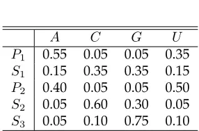
2.3 Emission probabilitiese(x|v). . . 56

2.4 Estimated emission probabilitiese(x|v)after 10 iterations. . . 57

3.1 The database search result for finding IREs. . . 82

4.1 Prediction results of the proposed method for several RNA families with pseudoknot structures. The prediction results of PSTAGs are also shown for comparison. The prediction results of PSTAGs are obtained from [66]. . . 111

4.2 CPU time for aligning two sequences in each RNA family. The experiments have been performed on a PowerMac G5 Quad 2.5 GHz with 4 GB memory. . . 111

4.3 Prediction results of the proposed method using randomly mutated RNA sequences. 112 6.1 Transition probabilities inside the CpG island region. . . 140

(20)

Chapter 1

Introduction

Signal processing is the art of representing, transforming, analyzing, and manipulating signals. It deals with a large variety of signals, including speech and audio signals, images and video signals, and even biological signals such as DNA sequences, ECG signals, MRI signals, and so forth. Signal processing techniques have been found useful in truly diverse applications, such as signal enhance-ment [33], denoising [14, 101], speech recognition [82], audio [73] and image compression [100, 118], radar signal processing [84], and digital communications [42, 43], just to name a few.

More recently, signal processing techniques have been also applied to the analysis of biological data with considerable success. For example, they have been utilized for the prediction of protein-coding genes [3, 106], characterization of ECG signals [63, 94], representation of gene regulatory networks [99], analysis of DNA microarray images [13, 115], and many others. The reader who is interested in the recent advances of signal processing methods in biology is referred to the following tutorial reviews [3, 22, 23, 112, 113, 130].

The primary focus of the thesis lies in the application of signal processing concepts to the anal-ysis of genomic sequence data. Among other things, this thesis presents various signal processing methods–such as digital filters, filter banks, and variants of HMMs (hidden Markov models)–that have been found especially useful in analyzing DNA and RNA sequence data and identifying re-gions of specific interest–e.g., protein-coding genes, CpG islands, and noncoding RNA (ncRNA) genes–inside these sequences. A more detailed outline of the thesis is presented in Section 1.6 of this Chapter.

(21)

order to serve this purpose. In Section 1.1 we briefly describe the discrete Fourier transform (DFT) that can be used for isolating the signal component with certain periodicity. The basic concepts of Markov chains and hidden Markov models (HMMs) are reviewed in Section 1.2 and Section 1.3, re-spectively. In Section 1.4, we review some fundamentals in genomics, and in Section 1.5, we briefly describe the concept of RNA secondary structures.

The material presented in this Chapter is only meant to be a quick introduction to signal pro-cessing and genomics, and it is by no means a complete and comprehensive coverage of these topics. For a more extensive treatment of these topics, the reader is referred to the references given at the end of each section.

1.1

Discrete Fourier transform (DFT)

Let us consider a finite length signalx(n)whose length isN. We assume thatx(n) = 0outside the range0≤n≤N−1. Thediscrete Fourier transform (DFT)ofx(n)is defined as

X[k] =

N−1

X

n=0

x(n)Wkn, (1.1)

whereW =e−j2π/N_{. Sometimes, we may assume that the signal}_x₍_n₎_{has length}_N _{even when its}

actual length is smaller. For example, it is possible thatx(n) = 0outside the range0 ≤n≤ L=

M −1, whereM ≤N. For this reason, the transform in (1.1) is sometimes called theN-point DFT, in order to prevent any ambiguity. As the Fourier transform ofx(n)is defined as

X(ejω) =X

n

x(n)e−jwn, (1.2)

we can view the DFTX[k]of a signalx(n)as a uniformly sampled version ofX(ejω₎_{at frequencies}

ωk = 2_Nπk fork = 0,1, . . . , N−1. Given the DFT coefficientsX[k], we can reconstruct the original

signalx(n)as follows

x(n) = 1

N

N−1

X

k=0

X[k]W−kn. (1.3)

(22)

opera-0 50 100 150 200 250 300 350 0

50 100 150 200 250 300 350

|X 1

[k]|

k

0 50 100 150 200 250 300 350 0

50 100 150 200 250 300 350

|X 2

[k]|

[image:22.612.154.494.109.376.2]

k

Figure 1.1: DFTs of periodic signals. (Top) Magnitude plot of the DFT of a signal with a period T = 3. (Bottom) Magnitude plot of the DFT of a signal with a periodT = 351/117.5.

tions, the FFT algorithm can compute the DFT in onlyO(NlogN)operations.1

The DFTX[k]of a signalx(n)can effectively analyze the frequency components contained in x(n). For example, the DFT coefficientX[k]shows the strength of the signal component whose frequency is located at (or near)ω = 2πk/N. This corresponds to the periodT =N/kin the time domain. Let us consider a finite-length periodic signalx1(n)defined as follows

x1(n) =ej2πn/3, 0≤n≤N−1, (1.4)

where the length of the signal isN = 351. As the period ofx1(n)if 3, its DFTX1[k] =DFT[x1(n)] should have a peak atω= 2π/3. This is demonstrated in Figure 1.1 (Top), where the magnitude of the DFTX1[k]has only a single peak atk=N/3 = 117. When the frequency of the input signal is not located at one of the frequenciesωk = 2_Nπk (k = 0,1, . . . , N −1), its energy will be distributed

(23)

0 50 100 150 200 250 300 350 0

50 100 150 200 250 300 350

|X3

[k]|

[image:23.612.187.462.95.323.2]

k

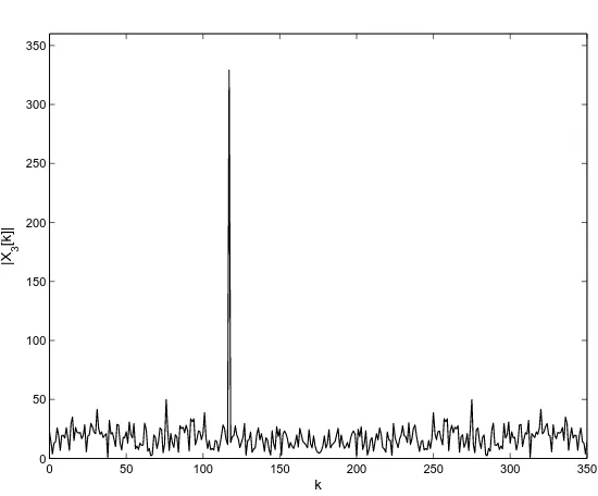
Figure 1.2: The DFT of a periodic signal with a periodT = 3buried in Gaussian noise. We can observe a clear peak atk=N/3.

over several frequency bins. For example, let us consider another periodic signalx2(n)defined as

x2(n) =ej2π(N/3)+0N .5n, 0≤n≤N−1,

whereN = 351is the same as before. The magnitude plot of the DFTX2[k] =DFT[x2(n)]is shown in Figure 1.1 (Bottom). We can see that the there are many non-zero DFT coefficients in this case, although the peak is located neark=N/3+0_N .5.

Finally, let us consider a periodic signal that is buried in noise. We define

x3(n) =x1(n) +z(n), 0≤n≤N−1

wherex1(n)is a periodic signal with periodT = 3as defined in (1.4) andz(n)is white Gaussian noise with unit variance. The magnitude plot ofX3[k] = DFT[x3(n)]is shown in Figure 1.2. In Figure 1.2, we can clearly observe the peak atk=N/3that corresponds to the periodT = 3of the signalx1(n).

(24)

1.2

Markov chain

Let us consider a system that can be described by one of a finite number of statesS={S1, . . . , SM}.

At each discrete time indexn, the stateynof the system takes one of the valuesyn ∈ S. The system

makes a state-transition at each unit time, which gives rise to a sequence of states

y0→y1→y2→. . .→yn. (1.5)

We say that this discrete-time stochastic process satisfies theMarkov property, if the probability distribution of the future stateyn+1depends only on the present stateynand not on the past states

yn−k(k≥1). This can be written as

P(yn+1=Sj|yn=Si, yn−1=Sk, yn−2=S`, . . .) =P(yn+1=Sj|yn=Si). (1.6)

In this case, the state sequence in (1.5) is called a first-order Markov chain (Markov model). If the transition probability shown in (1.6) is time independent such that

P(yn+1=Sj|yn=Si) =t(Si, Sj),

for alln, it is called astationaryMarkov chain. The transition probabilitiest(Si, Sj)satisfy

t(Si, Sj) ≥ 0 (1≤i, j≤M), M

X

j=1

t(Si, Sj) = 1 (1≤i≤M).

As we can see from above, a stationary Markov chain is completely governed by its state transition probabilitiest(Si, Sj), and it can be conveniently represented by a state transition diagram. An

example of such a diagram is shown in Figure 1.3. Unless mentioned otherwise, we assume that the Markov chain that is being used is stationary.

(25)

S

₁

S

₂

t(S₁,S₁)

t(S₁,S₂)

t(S₂,S₂)

t(S₂,S₁)

Figure 1.3: Example of a state transition diagram that represents a Markov chain with two distinct statesS1andS2.

Given that the current state isy0∈ S, how can we compute the probability that the nextLstates will be exactlyy1y2. . . yL? Using the Markov property, this probability can be simply computed as

P(y1y2. . . yL|y0) =

L

Y

n=1

P(yn|yn−1)

=

L

Y

n=1

t(yn−1, yn). (1.7)

Consider the case when we have multiple Markov chains, where each model describes the behavior of a system under different conditions. In this case, we can use the observation probability in (1.7) to determine which model describes the observed events best.

The Markov chains are utilized in Chapter 6, where they are used to represent the base se-quences inside CpG islands and those outside CpG islands. It is demonstrated that they can be effectively used for discriminating CpG islands from the non-CpG island regions. For further de-tails on Markov chains, the reader is referred to [89].

1.3

Hidden Markov model (HMM)

(26)

as follows. Letxn ∈ Abe the observed symbol at timen, whereA ={a1, . . . , aN}is the set of all

observable symbols. We denote the underlying state at timenasyn∈ S, whereS ={S1, . . . , SM}

is the set of distinct states in the hidden Markov model. As the state sequence satisfies the Markov property, we have

P(yn+1=Sj|yn =Si, yn−1=Sk, . . .) = P(yn+1=Sj|yn=Si)

= t(Si, Sj).

At timen, the emission probability of the observed symbolxndepends on the hidden stateyn

P(xn=ak|yn=S`) =e(ak|S`).

Note thatt(Si, Sj)is the stationary state transition probability from stateSito stateSj, ande(ak|S`)

is the stationary symbol emission probability of symbolak at stateS`. The stochastic process of

hidden states and the process of observable symbols are illustrated in Figure 1.4. In general, the hidden state sequence (typically called a “path”) cannot be directly inferred from the observed symbol sequence, although some information about the state sequence can be obtained from the observation. An HMM is completely defined by the set of parametersΘ = {T, E, π}, where the matricesT ={tij}andE={e`k}and the vectorπ={πi}are defined as follows.

tij = t(Si, Sj),

e`k = e(ak|S`),

πi = P(y1=Si),

for 1 ≤ i, j, ` ≤ M and 1 ≤ k ≤ N. T is the transition probability matrix, E is the emission probability matrix, andπis the initial state distribution of the model.

(27)

y₁

t(y₄,y₅)

y₂ y₃ y₄ y₅

x₁ x₂ x₃ x₄ x₅

t(y₃,y₄) t(y₂,y₃)

t(y₁,y₂)

… e(x1|y1) e(x2|y2) e(x3|y3) e(x4|y4) e(x5|y5)

observed symbols

[image:27.612.151.494.343.621.2]

hidden states

Figure 1.4: Illustration of the doubly embedded stochastic process in HMMs. The stochastic process consists of an observable symbol sequence and a hidden state sequence.

S

₁

S

₂

0.3

0.7

0.3

S

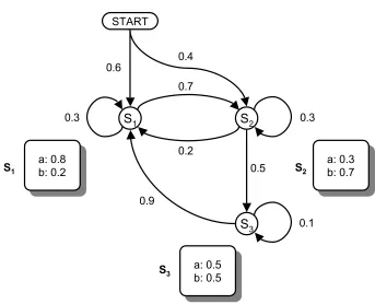
₃ 0.2

0.5

0.1 0.9

a: 0.8 b: 0.2

a: 0.8

b: 0.2 a: 0.3_{b: 0.7}

a: 0.3 b: 0.7

a: 0.5 b: 0.5

S1 S2

S3 START

0.4 0.6

(28)

set of parametersΘ ={T, E, π} T =     

0.3 0.7 0.0

0.2 0.3 0.5

0.9 0.0 0.1      , E =     

0.8 0.2

0.3 0.7

0.5 0.5      ,

π = h 0.6 0.4 0.0 i

.

As an example, let us consider the following observation sequence x with the underlying state sequenceyas shown below

x = a a b b a,

y = S1 S1 S2 S3 S1.

The probabilityP(x,y)can be computed as

There are three important problems that have to be solved in order to apply the HMMs to real world applications. These problems are typically called thealignment problem, thescoring problem, and thetraining problem. These problems are described in the following.

Alignment problem

Given an observed symbol sequencex=x1x2. . . xL and an HMM defined by the set of

pa-rametersΘ, how can we find the optimal state sequencey =y1y2. . . yLthat maximizes the

(29)

way [116]. The complexity of the Viterbi algorithm is onlyO(LM2), which increases linearly with respect to the sequence lengthL, whereM is the number of states.

Scoring problem

Given an observed symbol sequencex = x1x2. . . xL, how can we compute its observation

probability based on a given model Θ? As this probability can be used to score different models to choose the one that best describes the observation sequence, it is usually called the “scoring problem.” This problem can be efficiently solved using theforward algorithm[56, 81], which is closely related to the Viterbi algorithm. The complexity of the forward algorithm is alsoO(LM2₎_.

Training problem

Finally, we have to address the problem of how to choose the model parameters in an optimal manner, based on a number of training sequences. One popular solution to this problem is an EM (expectation-maximization) algorithm called the Baum-Welch algorithm [6]. This algorithm can iteratively find the parameters that achieve a local maximum of the observation probability of the training sequences.

The algorithms that can be used for solving these problems for HMMs are described in consid-erable detail in [56, 81].

HMMs are well known for their effectiveness in modeling short-term dependencies between adjacent symbols. For this reason, they have been extensively used in various fields, including speech recognition [56, 81] and bioinformatics [28, 59]. In Chapter 2, we extend the traditional HMM so that we can also describe long-range correlations between distant symbols. The extended model, called the context-sensitive HMM (csHMM) has important applications in RNA sequence analysis, as will be demonstrated in Chapter 3 and Chapter 4.

1.4

Review of some fundamentals in genomics

(30)

1.4.1

DNA and RNA

DNA (deoxyribonucleic acid) is a nucleic acid that contains the genetic information for cellular life forms and viruses. They are responsible for propagating the hereditary information in all living organisms. A single strand of DNA consists of many nucleotides that are linked to each other forming a long chain. A nucleotide consists of a base, a sugar, and a phosphate (or a phosphate group). The structure of a nucleotide is illustrated in Figure 1.6. The nucleotides that form a DNA strand can have four different kinds of bases, namely,adenine,cytosine,guanine, andthymine. For convenience, these nucleotides (or the bases) are typically represented by the four letters A, C, G, and T.

In general, a single strand of DNA forms adouble helixwith another single strand of DNA via hydrogen bonding between the bases. An illustration of a DNA double helix is shown in Figure 1.7. The nucleotide A in one strand is linked to T in the other strand (and vice versa), and the nucleotide C in one strand is connected to G in the other strand (and vice versa). As a result, one strand in a DNA double helix completely determines the nucleotide sequence in other strand, hence they are calledcomplementary strands.

Figure 1.8 shows an example of a short DNA double helix that has been straightened out for simplicity. As indicated in the figure, the sugar-phosphate forms the backbone of each DNA strand, and the two strands that run towards opposite directions are linked to each other by the chemical bonds formed between the complementary bases. As the nucleotide sequence in one strand deter-mines the nucleotide sequence in the other strand, a double-stranded DNA can be unambiguously represented by either strand. For this reason, a DNA molecule is represented by the nucleotide sequence of the forward strand, which is read from the so-called 5’-end to the 3’-end. For example, let us consider the DNA shown in Figure 1.8:

50−A−A−T−C−G−G−C−T −A−C−30 (forward strand)

30−T−T−A−G−C−C−G−A−T−G−50 (backward strand).

This can be simply represented by the forward strand

50−A−A−T−C−G−G−C−T−A−C−30.

(31)

se-A

5’

3’ 5’

G phosphate

sugar

base

nucleotide

A T C

DNA strand

[image:31.612.192.463.349.667.2]

3’

Figure 1.6: Illustration of a nucleotide and a DNA strand.

A T

G C

G

T A

C G

T A

C G

T A

G C

T A

C

G C

A T

sugar-phosphate

backbone

3.4nm

(34A)

(32)

A T C G A T C G A T C G C G A T _A T C G 5’ 3’ 3’ 5’ sugar-phosphate backbone bases forward strand backward strand

Figure 1.8: Example of a DNA double helix that has been straightened out for simplicity.

quence, where the symbols are taken from a finite alphabet.

The RNA (ribonucleic acid) is another type of nucleic acid that is closely related to the DNA. It also consists of four kinds of bases like the DNA, except thaturacil(U) is used instead of thymine (T). Unlike DNA molecules, the RNA is typically a single-stranded molecule.

1.4.2

Protein synthesis

A protein is a complex biomolecule that consists of a long chain of amino acids. The amino acids are linked to each other by strong covalent bonding called peptide bonds, and the amino acid chain is also known as a polypeptide. There are 20 different kinds of amino acids in proteins, where each amino acid has a different side-chain. Therefore, a protein can be conveniently represented as a sequence of amino acids, where each of the 20 distinct amino acids is denoted by a 3-letter code or an 1-letter code. For example, the amino acidalanineis denoted by ‘Ala’ or ‘A,’ andcysteineis denoted by ‘Cys’ or ‘C.’

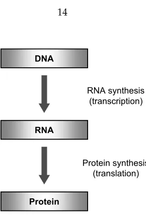
Proteins are involved in every single biological process in all cells, hence playing a crucial role in all living organisms. The information that is needed for encoding proteins is stored in the DNA. Portions in the DNA that contain the information for producing proteins are calledprotein-coding genes, or often simplygenes.2 Each gene in the DNA is first copied into an RNA molecule ( transcrip-tion), which is then used to produce proteins (translation). Therefore, it can be said that the genetic information flows from DNA to RNA to protein. This basic principle is typically called thecentral dogmaof molecular biology [1], and it explains how the genetic instructions contained in the DNA are used to synthesize RNAs and proteins. Figure 1.9 illustrates this principle in a simple diagram. The main steps in a typical protein synthesis process are shown in Figure 1.10. Each step in the process is discussed in the following subsections.

2_{Note that there exist also}_{ncRNA (noncoding RNA) genes}_{, which are portions of DNA that give rise to functional RNAs}

(33)

DNA

RNA

Protein

RNA synthesis (transcription)

[image:33.612.262.407.65.279.2]

Protein synthesis (translation)

Figure 1.9: The central dogma of molecular biology states that the genetic information flows from DNA to RNA to protein.

1.4.2.1 Transcription

The process of copying the content of a gene into an RNA is calledtranscription. The transcription process is carried out by an enzyme calledRNA polymerase, where anenzymeis a protein that cat-alyzes a specific chemical reaction. Initially, the RNA polymerase binds to a special region in the DNA called thepromoter, which is located upstream of a gene and is used to designate the starting point of the transcription process. During transcription, the RNA polymerase uses one strand of the DNA (called thetemplate strand) to copy the content into an RNA molecule. While copying the content from DNA to RNA, a thymine (T) in the original DNA sequence is replaced by a uracil (U) in the RNA that is being synthesized. The resulting transcript of a protein-coding gene is called a

pre-mRNA(pre-messenger RNA).

Living organisms can be categorized into two types, namely,prokaryotesandeukaryotes. Prokary-otes are simple organisms (mostly unicellular) that do not have a cell nucleus. Bacteria are com-mon examples of prokaryotes. On the other hand, eukaryotes are organisms that have complex cells with membrane-bound nuclei. Most of them are multicellular, and higher organisms such as worms, plants, insects and mammals belong to eukaryotes. Most protein-coding genes in eukary-otes consist of two types of regions called exons and introns (see Figure 1.10).3 _{The introns are} removed from the pre-mRNA and the remaining exons are concatenated to form amRNA (messen-ger RNA). This process is calledsplicing. Sometimes, one pre-mRNA gives rise to multiple mRNAs

(34)

Exon 1 Intron Exon 2 Intron Exon 3

5’ UTR 3’ UTR

Gene A Gene B Gene C

DNA

Pre-mRNA

mRNA

Exon 1 Exon 2 Exon 1 Exon 3

Protein

Protein 1 Protein 2

(a)

(b)

(c)

(d)

mRNA 1 mRNA 2

Transcription

Splicing

Translation

(35)

UUU : Phenylalanine UUC : Phenylalanine UUA : Leucine UUG : Leucine

CUU : Leucine CUC : Leucine CUA : Leucine CUG : Leucine

AUU : Isoleucine AUC : Isoleucine AUA : Isoleucine AUG : Methionine, Start

GUU : Valine GUC : Valine GUA : Valine GUG : Valine

UCU : Serine UCC : Serine UCA : Serine UCG : Serine

CCU : Proline CCC : Proline CCA : Proline CCG : Proline

ACU : Threonine ACC : Threonine ACA : Threonine ACG : Threonine

GCU : Alanine GCC : Alanine GCA : Alanine GCG : Alanine

UAU : Tyrosine UAC : Tyrosine UAA : Stop UAG : Stop

CAU : Histidine CAC : Histidine CAA : Glutamine CAG : Glutamine

AAU : Asparagine AAC : Asparagine AAA : Lysine AAG : Lysine

GAU : Aspartic acid GAC : Aspartic acid GAA : Glutamic acid GAG : Glutamic acid

UGU : Cysteine UGC : Cysteine UGA : Stop UGG : Tryptophan

CGU : Arginine CGC : Arginine CGA : Arginine CGG : Arginine

AGU : Serine AGC : Serine AGA : Arginine AGG : Arginine

GGU : Glycine GGC : Glycine GGA : Glycine GGG : Glycine

Figure 1.11: The genetic code.

by combining different exons. This phenomenon is calledalternative splicing, and it is widely ob-served in eukaryotes.

1.4.2.2 Translation

During thetranslationprocess, the mRNA that was transcribed from DNA is decoded by the ribo-some andtRNAs(transfer RNA) to generate a polypeptide (or a protein). A polypeptide is a long sequence of amino acids that are interconnected via peptide bonds. The translation of mRNAs into proteins is governed by thegenetic codethat maps each of the 64codons(triplets of nucleotides) into one of the 20 different amino acids. Figure 1.11 shows the genetic code that holds true for most genes in the vast majority of organisms. However, deviations from the standard code shown in Figure 1.11 are also widespread. For example, in several human mitochondrial mRNAs, the triplet ‘UGA’ was observed to code a tryptophan instead of serving as a stop codon [11].

(36)

(a) 5’ A C G A A A C G U C C A A A G C U U G 3’ A 5’ A A C G G C U A G 3’ A C U A U A G C C (b) A G A A A A 5’ U U C G

A G C U C G 3’ G C U A

5’ U U C G A A A G C U C G A A A A G G C U 3’ stem

loop

stem-loops

pseudoknot

Figure 1.12: Two examples of RNAs with secondary structures. The primary sequence of each RNA is shown along with its structure after folding. The dashed lines indicate interactions between bases. (a) RNA with two stem-loops. (b) RNA with a pseudoknot.

1.5

RNA secondary structure

As mentioned earlier, the RNA is a nucleic acid that consists of a chain of nucleotides. There are four distinct types of nucleotides, A, C, G, and U, where U is chemically similar to T. Just like in the DNA, A and U can form a hydrogen-bonded base pair, and similarly, C and G can also form a pair.4 In general, the RNA is a single-stranded molecule. If there exist complementary parts in a given RNA, these parts can form contiguous base pairs, making the RNA fold onto itself intramolecu-larly. This complementary base pairing determines the three-dimensional structure of the RNA to a considerable extent, and the two-dimensional structure resulting from the base pairing is referred as theRNA secondary structure. In contrast, the one-dimensional string of nucleotides is sometimes called theprimary sequenceof the RNA.

(37)

display characteristic secondary structures after folding. As indicated in Figure 1.12 (a), the con-tiguous base pairs that are stacked onto each other after folding is called astem, and the sequence of unpaired bases bounded by base pairs is called aloop. The secondary structure of the RNA in Fig-ure 1.12 (a) consists of twostem-loops(orhairpins). In many cases, the base pairings occur in a nested manner, where no interactions between bases cross each other. To be more precise, consider a base pair between locationsiandj(i < j), and another base pair between locationskand`(k < `). We say that these two base pairs are nested if they satisfyi < k < ` < j ork < i < j < `. The RNA shown in Figure 1.12 (a) has only nested interactions. Secondary structures with crossing interac-tions, where there exist base pairs at(i, j)and(k, `)that satisfyi < k < j < `ork < i < ` < j, are calledpseudoknots. One such example is shown in Figure 1.12 (b). Although RNA pseudoknots are observed less frequently than secondary structures with only nested base pairs, there are still many RNAs that are known to contain functionally important pseudoknots [104].

Many interesting RNAs are known to conserve their secondary structures among different species [25]. The conserved secondary structure gives rise to complicated long-range correlations between distant bases in the primary sequence of an RNA. More detailed discussion on this topic will be presented in Chapter 3.

For additional details on RNA secondary structures and RNA sequence analysis, the reader is referred to [25, 30].

1.6

Outline of the thesis

This thesis is organized as follows.

1.6.1

Context-sensitive hidden Markov models (Chapter 2)

In many applications, biological sequences are often treated as unstructured one-dimensional sym-bol sequences. However, they usually have higher dimensional structures that play important roles in carrying out their biological functions within cells. For example, an RNA molecule often folds onto itself to form a specific RNA secondary structure as shown in Section 1.5. This structure gives rise to complicated long-range correlations between distant bases in the RNA, which cannot be handled by simple models such as the Markov chains and the hidden Markov models (HMMs).

(38)

used for representing symbol sequences with long-range correlations. The csHMM is an exten-sion of the traditional HMM, where the emisexten-sion probabilities and the transition probabilities at certain states depend on the previous emission, called the “context.” This context-sensitive prop-erty increases the descriptive power of the model tremendously, making the csHMMs capable of handling complicated correlations between nonadjacent symbols. Due to the increased descrip-tive power of the model, we cannot use the algorithms that have been utilized for analyzing the traditional HMMs (e.g., the Viterbi algorithm, the forward algorithm, and the Baum-Welch algo-rithm). In Chapter 2, we propose dynamic programming algorithms that can be used with csHMMs for finding the optimal state sequence (the “alignment problem”) and computing the observation probability (the “scoring problem”) of a symbol sequence. In addition to this, we also propose a parameter reestimation algorithm that can be used for finding the optimal parameters of a csHMM based on a set of training sequences.

1.6.2

RNA sequence analysis using context-sensitive HMMs (Chapter 3)

The context-sensitive HMMs proposed in Chapter 2 have important applications in RNA sequence analysis. In Chapter 3, we focus on the role of csHMMs in the computational identification and analysis of the so-called noncoding RNAs (ncRNAs). For a long time, it has been believed that pro-teins are responsible for most of the important biological functions within cells. In the meanwhile, the RNA was mainly viewed as a passive intermediary that interconnects DNA and proteins. How-ever, recent results indicate that ncRNAs, which are RNA molecules that function without being translated into proteins, play pivotal roles in various biological processes, especially in controlling the regulatory mechanisms in the cells [30, 44].

In Chapter 3, we show how the csHMMs can be utilized for building probabilistic representa-tions of ncRNA families and finding new ncRNA genes. We give examples of csHMMs that repre-sent the correlations in symbol sequences that arise from various RNA secondary structures. Then, we propose a dynamic programming algorithm that can be used for searching a large database to find similar sequences that closely match the original RNA that is represented by the csHMM at hand.

(39)

ex-pression level of certain genes. Alternative folding in RNAs introduces some complications, as the resulting correlation structure is significantly more complex than those of typical RNAs that take only one structure. At the end of Chapter 3, we propose a method based on csHMMs, which can be used for modeling and identifying RNAs with alternative secondary structures. The pro-posed method provides a good prediction performance at a reasonably low complexity, making it practically usable in real applications.

The main emphasis of Chapter 3 lies on building tools that can be used to find new members (or homologues) of known ncRNA families.

1.6.3

Profile context-sensitive hidden Markov models (Chapter 4)

In Chapter 4, we present a subclass of context-sensitive HMMs, called profile-csHMMs, which are especially useful in representing RNA profiles. The Profile-csHMM is a csHMM with a linear structure that repetitively uses three kinds of states, namely, match states, delete states, and insert states. Unlike traditional profile-HMMs, some of the match states are made context sensitive such that we can represent pairwise correlations between the bases that form a complementary base pair in the RNA secondary structure. Profile-csHMMs can be easily constructed from an RNA multiple sequence alignment, in a simple and intuitive manner.

One of the most important advantages of profile-csHMMs is that they are capable of model-ing any kind of RNA pseudoknots. For example, models such as CMs (covariance models) [26] that have been extensively used for modeling RNAs, can only describe nested correlations, hence not capable of handling pseudoknots. More recent models such as PSTAGs (pair stochastic tree adjoining grammars) [66] can also deal with many pseudoknots, but not all of them. Based on profile-csHMMs, we propose a dynamic programming algorithm, which is called the sequential component adjoining (SCA) algorithm, that can be used for finding the optimal state sequence of profile-csHMMs.

(40)

Finally, we consider the problem of performing an RNA homology search using profile-csHMMs. Although the profile-csHMM alignment algorithm runs reasonably fast, it is still slow if we want to use it for scanning a large database. At the end of Chapter 4, we propose an efficient pre-filtering scheme for making a profile-csHMM search significantly faster, without affecting its prediction accuracy.

1.6.4

Predicting protein-coding genes using digital filters (Chapter 5)

In Chapter 5, we present digital filtering methods for identifying protein-coding genes. It is well known that protein-coding regions in DNA sequences frequently display period-3 behaviors that are not observed in noncoding regions. Therefore, we can exploit this property for identifying protein-coding regions in a given DNA sequence. Traditionally, these regions have been identified with the help of windowed DFT (discrete Fourier transform) [3, 106]. From a digital filtering per-spective, we can view the DFT approach as digital filtering using a bandpass filter whose passband is centered at2π/3. In this way, we can extract the period-3 component to measure the strength of the periodic behavior in a specific region. However, the DFT-based filter does not have a high stopband attenuation, which leaves a considerable amount of undesirable noise after filtering.

We can overcome this problem by designing a better digital filter with a higher stopband attenu-ation. In Chapter 5, we propose two different methods for designing digital filters that can be used for identifying protein-coding genes. The first method is based on allpass-based antinotch filters and the second method is based on multistage digital filtering. Experimental results indicate that both methods can isolate the period-3 components from the noisy background considerably better than the traditional DFT approach. Furthermore, the digital filters that are used in the proposed methods can be very efficiently designed, providing a significant advantage in terms of computa-tional cost.

(41)

1.6.5

Identification of CpG islands using filter banks (Chapter 6)

The CpG islands are specific regions in DNA molecules that are abundant in the dinucleotide CpG. They are usually located upstream of the transcription start regions of many genes, hence can be used as good gene markers. Furthermore, the methylation of CpG islands is known to play an important role in gene silencing, genomic imprinting, carcinogenesis, and so forth. For this reason, the computational identification of CpG islands has been of interest to many researchers.

(42)

Chapter 2

Context-Sensitive Hidden Markov

Models

Although biological sequences are often treated as unstructured one-dimensional symbol sequences for simplicity, they usually have three-dimensional structures that play important roles in carrying out their biological functions in cells. For example, a polypeptide (a long chain of amino acids) is biologically inactive until it folds into a correct three-dimensional protein structure. This is typi-cally calledprotein folding[11]. RNAs, which usually exist as single-stranded molecules, often fold onto themselves intramolecularly to form consecutive base-pairs. The three-dimensional structure of an RNA is determined by this complementary base-pairing to a considerable extent, and the two dimensional structure that results from this base-pairing is referred as theRNA secondary struc-ture[25].1 Due to these structures, many biological sequences–such as proteins and noncoding RNAs (ncRNAs)– exhibit complicated correlations between nonadjacent symbols [25]. Such corre-lations cannot be effectively handled by simple models such asMarkov chainsandhidden Markov models (HMMs). In fact, these models belong tostochastic regular grammars (SRGs)according to the so-calledChomksy hierarchy of transformational grammars, which cannot model symmetric sequences (orpalindromes). As RNAs with conserved secondary structures can be viewed as “biological palin-dromes,” these models are incapable of handling RNA sequences. This will be described in more detail in Section 2.2.

In order to overcome this limitation, we propose a new statistical model in this chapter, which is called the context-sensitive hidden Markov model (csHMM). The csHMM is an extension of the conventional HMM, where the probabilities at some states are made context sensitive. This in-creases the descriptive capability of the model tremendously, making csHMMs capable of

(43)

ing long-range correlations between nonadjacent symbols.2 _{The proposed model has several} ad-vantages over other existing models, including the stochastic context-free grammars (SCFG), as will be demonstrated later. The csHMMs are especially useful for modeling ncRNAs with conserved secondary structures and for building RNA sequence analysis tools.

The content of this chapter is mainly drawn from [131], and portions of it have been presented in [123, 127, 128].

2.1

Outline

The organization of this chapter is as follows. In Section 2.2, we briefly review the Chomsky hierar-chy of transformational grammars, and explain where the conventional HMMs are located in this hierarchy. We show that the descriptive capability of HMMs is limited to sequences with sequential dependencies and give examples that cannot be effectively modeled by the HMMs.

In Section 2.3, we introduce the concept of context-sensitive HMM (csHMM), which is an ex-tension of the HMM that can be used for representing long-range correlations between distant symbols. We first elaborate on the basic elements of a csHMM in Section 2.3.1, and explain in Section 2.3.2 how these elements can be used to build an actual csHMM.

In Section 2.4, we consider the “alignment problem” of csHMMs. It is shown that the Viterbi algorithm cannot be used for finding the optimal state sequence of a csHMM due to the context-sensitive property of the model. In Section 2.4.1, we briefly describe how we can implement a dynamic programming algorithm that can be used for finding the optimal state sequence that max-imizes the probability of an observation sequence, based on a given csHMM. The algorithmic de-tails are described in Section 2.4.2 and Section 2.4.3, and the overall complexity of the algorithm is analyzed in Section 2.4.4.

The “scoring problem” of csHMMs is considered in Section 2.5. In this section, we show how we can compute the observation probability of a symbol sequence in a systematic way. The details of the scoring algorithm is described in Section 2.5.1. In addition to this, we describe the outside algorithm for csHMMs in Section 2.5.2, which can be used along with the scoring algorithm for estimating the model parameters of csHMMs.

In Section 2.6, we describe a parameter re-estimation algorithm for csHMMs. We can iteratively 2_{It has to be noted that the}_{context-sensitive HMMs}_{proposed in this chapter are not related to the so-called}

(44)

apply the proposed algorithm to train a csHMM based on a set of training sequences. Experimental results are given in Section 2.7, which demonstrate the effectiveness of the algorithms proposed in Section 2.4, Section 2.5, and Section 2.6.

In Section 2.8, we discuss several interesting issues related to csHMMs. For example, we con-sider extending the proposed model for representing non-pairwise correlations in Section 2.8.1 and explain how csHMMs can be used for modeling crossing correlations in Section 2.8.2. In Sec-tion 2.8.3, we compare the proposed model with other variants of HMMs. The csHMM is also com-pared to other transformational grammars (e.g., context-free grammars, context-sensitive gram-mars) in Section 2.8.4, and we show that csHMMs have several advantages over these grammars. Concluding remarks are given in Section 2.9.

Finally, in Appendix A, we give an example of a context-free grammar (CFG) that cannot be represented by a csHMM. As there also csHMMs that cannot be represented by CFGs (shown in Section 2.8.2), this demonstrates that neither the csHMMs nor the CFGs fully contain the other (see Figure 2.19). In Appendix B, we describe simplified versions of the alignment algorithm and the scoring algorithm that are proposed in Section 2.4 and Section 2.5, respectively. The simpli-fied algorithms can be used for analyzing sequences withsingle nested correlations, and they are computationally more efficient compared to the original algorithms.

2.2

HMMs and transformational grammars

Hidden Markov models (HMMs) have been widely used in many fields. They are well known for their efficiency in modeling short-term dependencies between adjacent symbols, which made them popular in diverse areas. Traditionally, HMMs have been successfully applied to speech recognition, and many speech recognition systems are built upon HMMs and their variants [56, 81]. They have been also widely used in digital communications, and more recently, HMMs have become very popular in computational biology as well. They have been proved to be useful in various problems such as gene identification [25, 58, 96], multiple sequence alignment [25, 27], and so forth. Due to its effectiveness in modeling symbol sequences, the HMM gave rise to a number of useful variants that extend and generalize the basic model [35, 49, 50, 70, 79, 80, 136].

(45)

Type Allowed production rules

Regular Grammar A−→aB|a|

Context-Free Grammar A−→α

Context-Sensitive Grammar αAγ−→αβγ or S−→ Unrestricted Grammar αAγ−→δ

Table 2.1: The Chomsky hierarchy of transformational grammars.

are distant from each other. Therefore, the resulting model always displays local dependencies,3 and more complex sequences with non-sequential dependencies cannot be effectively represented using the conventional HMMs.

2.2.1

Transformational grammars

In computational linguistics, atransformational grammaris defined as a set of rules that can be used to describe (or generate) a set of symbol sequences over a given alphabet. It was first formally proposed by the computational linguist Noam Chomsky [16]. A transformational grammar can be characterized by the following components: terminal symbols,nonterminal symbols, andproduction rules. Terminal symbols are the observable symbols that actually appear in the final symbol se-quence, and nonterminal symbols are abstract symbols that are used to define the production rules. A production rule is defined asα→β, whereαandβ are strings of terminal and/or nonterminal symbols. It describes how a given string can be transformed into another string. We can generate various symbol sequences by applying these production rules repetitively, where the generation process starts from the start nonterminalSand terminates when there are no more nonterminals.

As an example, let us consider the following grammar which has a single nonterminal{S}and two terminals{a, b}:

S−→aS, S−→b.

This simple grammar can generate any sequence of the forma . . . ab. For example, we can generate the sequenceaaabby applying the above rules as follows

S −→aS−→aaS−→aaaS−→aaab.

In his work on transformational grammars, Chomsky categorized transformational grammars 3_By_{local dependencies}_{, we imply that the probability that a symbol appears at a certain location depends only on its}

(46)

regular unrestricted

context-free context-sensitive

• more complex • more powerful • less restricted

Figure 2.1: The Chomsky hierarchy of transformational grammars nested according to the restric-tions on the allowed production rules.

into four classes. These are theregular grammars,context-free grammars,context-sensitive grammars

andunrestricted grammars, in the order of decreasing restrictions on the production rules. The pro-duction rules allowed in each class are summarized in the Table 2.1.AandBare single nontermi-nals,ais a single terminal, andis the empty sequence.α,γ,δare any string of terminals and/or non-terminals, andβ is any nonempty string of terminals and/or non-terminals. (The notation ’|’ means ’or.’) These four classes comprise the so-calledChomsky hierarchy of transformational gram-mars, which is illustrated in Figure 2.1. As can be seen from the diagram, regular grammars are the simplest among the four, and they have the most restricted production rules.

HMMs can be viewed as stochastic regular grammars (SRG), according to this hierarchy. Due to the restrictions on their production rules, regular grammars have efficient algorithms such as the

(47)

aaba

abaa

babba

abbab

Figure 2.2: Examples of sequences that are included in the palindrome language. The lines indicate the pairwise correlations between distant symbols.

2.2.2

Palindrome language

One interesting language that cannot be represented using regular grammars (or equivalently, us-ing HMMs) is thepalindrome language[16]. The palindrome language is a language that contains all strings that read the same forwards and backwards. For example, if we consider a palindrome language that uses an alphabet of two letters{a, b}forterminal symbols, it contains all symbol se-quences of the formaa,bb,abba,aabbaa,abaaba, and so on. Figure 2.2 shows examples of symbol strings that are included in this language. The lines in Figure 2.2 that connect two symbols indicate the pairwise correlations between symbols that are distant from each other. Similarly, RNAs with conserved secondary structures display long-range correlations between nonadjacent bases, due to the existence of symmetric (orreverse complementary, to be more precise) portions in their pri-mary sequences. This kind of long-range interactions between symbols cannot be described using regular grammars.

It is of course possible that a regular grammar generates such palindromes as part of its lan-guage. However, we cannot force the model to generateonly such palindromes. Therefore regular grammars are not able to effectively discriminate palindromic sequences from non-palindromic ones. In fact, in order to describe a palindrome language, we have to use higher-order grammars such as the context-free grammars. Context-free grammars are capable of modeling nested depen-dencies between symbols that are shown in Figure 2.2.

(48)

2.3

Context-sensitive hidden Markov models

The context-sensitive HMM can be viewed as an extension of the traditional HMM, where some of the states are equipped with auxiliary memory [123, 131]. Symbols that are emitted at certain states are stored in the memory, and the stored data serves as thecontextthat affects the emission probabilities and the transition probabilities at certain future states. This context-sensitive property increases the descriptive power of the model significantly, compared to the traditional HMM. Let us first formally define the basic elements of a context-sensitive HMM.

2.3.1

Basic elements of a csHMM

Similar to the traditional HMMs, the csHMM is also adoubly-stochastic process, which consists of a non-observable process of hidden states and a process of observable symbols. The process of the hidden states is governed by state-transition probabilities that are associated with the model, and the observation process is linked to the hidden process via emission probabilities of the observed symbol that is conditioned on the hidden state. A csHMM can be characterized by the following elements.