Optimization of windspeed prediction using an artificial neural network compared with a genetic programming model

328

Chapter 15

ABSTRACT

The precise prediction of windspeed is essential in order to improve and optimize wind power predic-tion. However, due to the sporadic and inherent complexity of weather parameters, the prediction of windspeed data using different patterns is difficult. Machine learning (ML) is a powerful tool to deal with uncertainty and has been widely discussed and applied in renewable energy forecasting. In this chapter, the authors present and compare an artificial neural network (ANN) and genetic programming (GP) model as a tool to predict windspeed of 15 locations in Queensland, Australia. After performing feature selection using neighborhood component analysis (NCA) from 11 different metrological parameters, seven of the most important predictor variables were chosen for 85 Queensland locations, 60 of which were used for training the model, 10 locations for model validation, and 15 locations for the model test-ing. For all 15 target sites, the testing performance of ANN was significantly superior to the GP model.

Optimization of Windspeed

Prediction Using an Artificial

Neural Network Compared With

a Genetic Programming Model

University of Southern Queensland, Australia

Sujan Ghimire

University of Southern Queensland, Australia

Nathan J. Downs

University of Southern Queensland, Australia

Nawin Raj

Optimization of Windspeed Predictionl

1. INTRODUCTION

The fluctuation of the wind heavily affects wind power generation. Therefore, accurate wind forecast-ing models are very important for effective wind power systems management. Among all the renewable energy sources, windspeed needs more forecasting approaches than currently implemented due to its higher intermittency rate (Masrur, Nimol, Faisal, & Mostafa, 2016). In the literature, three different methods have been introduced for windspeed (Ws) forecasting: physical, statistical and hybrid (Foley, Leahy, Marvuglia, & McKeogh, 2012). Physical methods are based on principles of physics such as the numerical weather prediction (NWP) models. Statistical models can be as simple as persistence to more complicated models such as Artificial Neural Networks (ANN) (Blonbou, 2011) or Markov chains. Hybrid methods combine physical and statistical models like the Autoregressive Integrated Moving Av-erage Model (ARIMA) and ANN, which can generate non-linear functions to create an accurate model capable of predicting time series of windspeed and wind power output.

Many studies with several different models were done for diverse regions around the world. The ARIMA model was proposed by Benth and Benth (Benth & Benth, 2010) for forecasting the windspeed for three different wind farms in New York state. Zhu and Genton (Zhu & Genton, 2012) reviewed statistical short-term windspeed forecasting models, including autoregressive models and traditional time series approaches used in wind power developments to determine which model provided the most accurate forecasts. Due to the nonlinearity pattern of wind data, the forecasts using ARIMA may have inaccuracies because the ARIMA model is a linear series model (Cadenas & Rivera, 2010). Therefore, ANN has been applied to handle the nonlinear nature of windspeed data in previous research. A com-parison of ANN and ARIMA was presented by Cadenas and Rivera (Cadenas & Rivera, 2007) using seven years of windspeed data. Six years of this dataset were used for the training, and one year for the validation, using performance metrics like Mean Square Error (MSE) and Mean Absolute Error (MAE). These were found to be lower for ANN when compared with ARIMA. Similarly, daily, weekly and monthly windspeed was forecasted using data from four different measuring stations in the Aegean and Marmara regions of Turkey by Bilgili and Sahin (Bilgili & Sahin, 2013). The results show that the ANN forecast was superior. In addition to this, recently Zameer et al. (Zameer, Arshad, Khan, & Raja, 2017), proposed the Genetic Programming (GP) model for the short term prediction of wind for five different wind farms in Europe, the average root MSE was 0.1176 ms-1_.

Optimization of Windspeed Predictionl

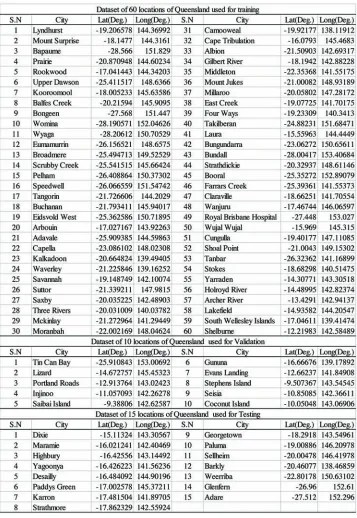
In our study, we have developed two ML models, ANN and GP to predict Ws for 15 locations in Queensland, Australia. ANN and GP is an appropriate method for wind power prediction and has been widely used (Alexiadis, Dokopoulos, Sahsamanoglou, & Manousaridis, 1998; Fan, Wang, Liu, & DAI, 2008; Kariniotakis, Stavrakakis, & Nogaret, 1996; Mohandes, Rehman, & Halawani, 1998; Seo & Hy-eon, 2015) in renewable energy prediction. In order to form the ML model, monthly average values of metrological parameters for 85 locations in Queensland were extracted from the surface meteorology and solar energy release 6.0 (SSE 6.0) (Stackhouse & Whitlock, 2009). This data was obtained from the NASA Science Mission Directorate’s satellite and re-analysis research programs which extends the temporal coverage of the solar and meteorological data from 10 years to more than 22 years. A total of 60 cities of the Queensland region were used for training, 10 cities for the validation and 15 cities for testing. Before feeding the ANN and GP model, feature selection was performed to optimize the selec-tion of predictor variables.

2. METHODOLOGY

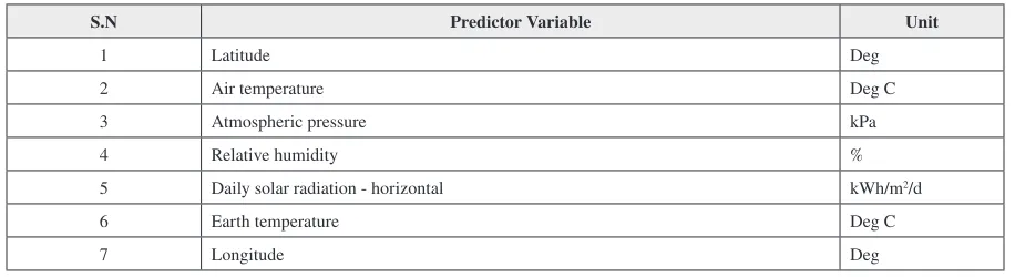
Table 1 shows the list of predictor variables extracted from SSE 6.0. Combinations of these variables were used for the long-term prediction of Ws. The monthly average values for each these variables were taken as input for the feature selection.

2.1 Artificial Neural Network

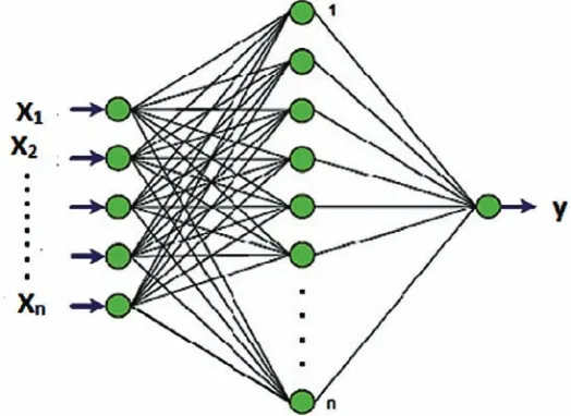
In this study, we applied an artificial neural network based multilayer perceptron (MLP) algorithm to examine the problem of windspeed forecast. Briefly, the MLP model is one of the most common neural network architectures, utilizing a feedforward backpropagation (FFBP) network. The basic advantages of ANN over the conventional correlations is neural networks have large degrees of freedom for fitting parameters and thus, capture the systems’ non-linearity better than regression methods. Furthermore, ANN can be further trained and refined when additional data become available in order to improve their

Table 1. Description of the extensive pool of predictor variables and notations

S.N. Predictor Variable Abbreviation Unit

1 Latitude Lat Deg

2 Longitude Long Deg

3 Elevation Elev m

4 Air temperature Tair Deg C

5 Relative humidity RH %

Optimization of Windspeed Predictionl

prediction accuracy while it is impossible to make any further change in a linear or non-linear regression model as soon as a model development is over (Farshad, Garber, & Lorde, 2000; Gharbi & Elsharkawy, 1996; Gharbi & Elsharkawy, 1997; Makinde, Ako, Orodu, & Asuquo, 2012). The FFBP model has been applied in many previous studies of renewable energy (e.g., Ravinesh C Deo & Sahin, 2017; Ghorbani, Khatibi, Hosseini, & Bilgili, 2013). The FFBP model offers a competent learning environment that mini-mizes error between the target and the obtained values (Ul-Saufie, Yahaya, Ramli, Rosaida, & Hamid, 2013). As shown in Figure 1 the network of FFBP usually consists of an input layer (X₁, X₂, X₃,..X_n), several hidden layers, and an output layer (Y). Each layer consists of several operating neurons, each of which is connected to every neuron in nearby layers through adaptable synaptic weights that determine the strength of the relationship between two connected neurons. In each layer, every neuron sums all the inputs that have been received from previous layers and forms the neuron output through a predefined activation or transfer function. Learning is defined as the ability of a network to change weights by ap-plication of a backpropagation algorithm through two phases. In the forward phase, the training data set is propagated through the hidden layer and comes out of the neural network through the output layer. The output values are then compared with actual target output values. The error between the output layer and the actual values are calculated and propagated back toward the hidden layer (Elbayoumi, Ramli, & Fitri Md Yusof, 2015). In the backward phase, derivatives of network error (with respect to the networks) are fed back to the network and used to adjust the weights to reduce errors with each iteration, thus improv-ing the FFBP models and promptimprov-ing the neural model to produce the desired outputs.

The network construction in this study consists of three-layer perceptron model. The first input layer contains the input variables that were selected by neighborhood component analysis (Yang, Wang, & Zuo, 2012) feature selection “fsrnca” method to reduce complexity by retaining fewer variables. The second architecture layer is the hidden layer. The common problems in hidden layer architecture are to identify the number of hidden layers, to identify neurons values and to choose the suitable activation function. The optimum number of neurons is important because too few neurons will contribute to

Optimization of Windspeed Predictionl

under-fitting, whereas too many neurons lead to overfitting. A fixed scientific solution for the design of an optimal ANN model does not exist. Using Equation 1, the initial number of neurons will be found and the number was increased until a stable and optimal value was achieved.

n_h = × +2 n_i 1

where, n_i is the number of input neurons, and n_h is the number of hidden neurons.

The second problem in building the architecture of the hidden layer is deciding suitable transfer func-tion. According to Kriesel (Kriesel, 2007), the transfer function in the hidden layers must use a nonlinear transfer function (otherwise the result end up with only linear separable solutions). Therefore, the optimal activation functions are obtained using sigmoid transfer function (Ul-Saufie, Yahaya, Ramli, Rosaida, & Hamid, 2013). The most common sigmoid functions are linear (purelin), log-sigmoid (logsig) and hyperbolic tangent sigmoid (tansig). The logistic function will generate values close to 0. If the argument of the function is negative, the output of hidden neuron will be close to zero, and as a result lowering the learning rate for all subsequent weights-will almost stop learning. Tansig can produce both positive and negative values which will generate a value close to −1.0, and thus will maintain learning (Kriesel, 2007). In this study, tansig, logsig and purelin functions were used to build the architecture of the hid-den layer. The third architecture layer is the output layer which consists of the target of the forecasting model which is the windspeed.

The ANN algorithm can be formulated as (REF):

Y X F w t X t_{i i} b

i L ( )=  ( ). ( )+        =

∑

1 2 1

1

1 ))

Linear=linear(x)=x

where X_i(t) is representing predictor/forecasting (input) variable(s) in discrete time space t while Y(x) is referred to a forecasted windspeed (Y) in (test) data set. Moreover, L is the number of hidden neurons that determined iteratively after finding the initial hidden neuron from Equation 1, w_j (t) is the weight which connects the ith _{neuron in the input layer. In Equation 2, b is used a neuronal bias and F(.) is the}

function of hidden transformation in the ANN network architecture.

Optimization of Windspeed Predictionl

Conjugate Gradient Backpropagation with Fletcher-Reeves Updates (traincgf) and Levenberg–Marquardt Backpropagation (trainlm) (MathWorks, 1996).

The traincgp algorithm, is the ratio of the inner product of the previous change in the gradient with the present gradient to the norm squared of the last gradient (Hagan, Demuth, & Beale, 1996; Møller, 1993), whereas the traincgf algorithm is the ratio of the norm squared of the current gradient to the norm squared of the previous gradient. In the first iteration, the conjugate gradient algorithm will find the steep descent direction. Approximate solution, ‘X_k’ for conjugate gradient iteration is described as formulas below (Ojha, Dutta, Chaudhuri, & Saha, 2013).

X_k =X_k+1+α_k·d_k

where, learning rate αk is determined using line search algorithm such that

SSE X( _k +α_{k k}g )≤SSE g( )_k

where, ‘d_k’ is the search direction basically d_k = −g_k, where g_k is gradient computed based on ‘X_k’. Note that,

d g k

g d Otherwise

k

k

k k k

= − =

− +    

 −

0

1

β

where, β_k is a factor which scales the influence previous gradient analogous to momentum factor in backpropagation.

The different methods employed in the computation of β_k leads to different versions of conjugate gradient methods.

For traincgf and traincgp, the β_k is calculated as per Equation [7] and Equation [8] respectively. Where, y_k−1=g_k −g_k−1:

β_k k k

g g

=

− 2

1 2

β_k k T

k

k

g y g

= −

− 1

1 2

Optimization of Windspeed Predictionl

The trainscg (Hagan, Demuth, & Beale, 1996; Møller, 1993) is formulated to avoid the time consump-tion in line search at each iteraconsump-tion of other conjugate gradient algorithms. It is used as general-purpose training algorithms.

The trainbfg algorithm approximates Newton’s method, a class of hill-climbing optimization tech-niques that seeks a stationary point of a function. For such problems, a necessary condition for optimality is that the gradient be zero (MathWorks, 1996).

The basic step of Newton’s method is:

X_{k+ =}X_{k −}A g_k− _k 1

1_.

where, A_k−1 _{is the Hessian matrix (second derivatives) of the performance index at the current values of}

the weights and biases. Newton’s method often converges faster than conjugate gradient methods. Un-fortunately, it is complex and expensive to compute the Hessian matrix for feedforward neural networks. There is a class of algorithms that is based on Newton’s method, but it does not require calculation of second derivatives. These are called quasi-Newton (or secant) methods. They update an approximate Hessian matrix at each iteration of the algorithm. The update is computed as a function of the gradient trainbfg updating method and the trainlm algorithms avoid this difficulty because they update an ap-proximate Hessian matrix at each iteration of the algorithm. Levenberg–Marquardt algorithm was de-signed to approach second-order training speed without having to compute the Hessian matrix. If the performance function has the form of a sum of squares, then the Hessian matrix can be approximated as (Sharma & Venugopalan, 2014). If the performance function has the form of a sum of squares, then the Hessian matrix can be approximated as:

H ₌J JT

and the gradient can be computed as:

g₌J eT

Where ‘J’ is the Jacobian matrix that contains first derivatives of the network errors with respect to the weights and biases, and ‘e’ is a vector of network errors. The Jacobian matrix can be computed through a standard back propagation technique that is much less complex than computing the Hessian matrix. The Levenberg–Marquardt algorithm uses this approximation to the Hessian matrix in the following Newton-like update:

X_k X_k J JT I J eT

+

−

= −_ + _

1

1

Optimization of Windspeed Predictionl

The trainbfg have superior performance even for non-smooth optimizations and an efficient train-ing function for smaller networks whereas the trainlm algorithm locates the minimum of a multivariate function that can be expressed as the sum of squares of non-linear real-valued functions. It is an iterative technique that works in such a way that performance function will always be reduced in each iteration of the algorithm. This feature makes trainlm back propagation optimization learning algorithm is the most rapid learning algorithm tool for moderate size network (Kamble, Pangavhane, & Singh, 2015). Both trainbfg and trainlm function has drawback of memory and computation overhead caused due to the calculation of the gradient and approximated Hessian matrix (Pham & Sagiroglu, 2001).

The trainoss algorithm is an improved method of trainbfg algorithm as it decreases the calculation and storage at each iteration. The trainoss method does not store the complete Hessian matrix; it assumes that the previous Hessian matrix was the identity matrix. This function has additional advantage that the new search direction can be calculated without computing a matrix inverse. So, trainoss is consid-ered a compromise between full quasi-Newton algorithms and conjugate gradient algorithms (Kamble, Pangavhane, & Singh, 2015).

2.2 Multi- Gene Genetic Programming

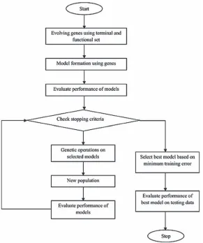
Genetic Programming (GP) uses principle of genetic algorithms (GA) to evolve computer programs/ models of varying sizes based on Darwinian Theory of “Survival of the fittest” (Koza, 1994). Although both GP and GA share the same working principle but there exists difference between them. The GP represents the problem solution as a tree in a symbolic form (Poli, Langdon, & McPhee, 2008; Raja, 2008) whereas GA evolves solutions represented by strings (binary or real number) of fixed length (Garg, Vijayaraghavan, Mahapatra, Tai, & Wong, 2014). Figure 2 below illustrates the main parts of GP approach. As shown, in the first step, the GP creates an initial population (individuals) based on a random search of space. Each individual, also called program, has a symbolic tree structure and is made up of predefined functions set and terminals. At next step, the fitness function is used to evaluate each individual of population. After that, with respect to the Darwinian principle (reproduction of the fit-test individual), the new generation will be created by using three genetic operators, namely crossover, mutation and reproduction.

The most common method of recombination is crossover. In this method two parents swap randomly selected sub-trees to produce two children. Mutation involves replacing the sub-tree with a new randomly generated tree at a mutation point. Reproduction selects the fitter individuals and repeats them into next generation with no change. After applying genetic operators, the new population is evaluated for fitness. This process will continue until criterion is satisfied that is finding the optimized individual, or reaching predefined number of generations. Another important aspect in GP is choosing the individuals for recombination. Different methods for individual selection have been proposed. The two common methods are fitness selection and tournament selection. In first method, each individual has a chance to be selected in accordance with its fitness, whereas in the second method, a small number of individuals compete in a fitness tournament to be selected for recombination (Rahdari, Eftekhari, & Mousavi, 2016).

Optimization of Windspeed Predictionl

A free open source GP toolbox called “GPTIPS “software is used for the implementation of GP. This software is a new “Genetic Programming and Symbolic Regression” code written based on MGGP (Hinchliffe, Hiden, McKay, Willis, Tham, & Barton, 1996; Searson, Leahy, & Willis, 2010) for the use with MATLAB (MathWorks, 1996). In GPTIPS, there are some adjustable parameters like the maximum number of genes in the regressing process, primary mathematical operators, number of population and so on which should be determined before the run by user. The structure of multigene symbolic regres-sion models is illustrated in Figure 3.

The prediction of the y training data is given by:

ˆ ...

y=b₀+b t_{1 1}+ +b t_{G G}

where t_i is the (N × 1) vector of outputs from the ith _{tree/gene comprising a multigene individual. Next,}

define G as a (N × (G + 1)) gene response matrix as follows in Equation [14].

G =[ ... ]1t₁ t_g

where, the 1 refers to a (N × 1) column of ones used as a bias/offset input. Now, Equation [13] can be written as:

ˆ

y=Gb

The least squares estimate of the coefficients b₀, b₁, b₂,..., b_G formulated as a ((G + 1) × 1) vector can be computed from the training data as Equation [16]:

b₌₍G G G yT ₎−1 T

In practice, the columns of the gene response matrix G may be collinear (e.g. due to duplicate genes in an individual, and so the Moore-Penrose pseudo-inverse (by means of the singular value decomposition; SVD) is used in Equation [16] instead of the standard matrix inverse. Because this is computed for every individual in a GPTIPS population at each generation (except for cached individuals), the computation of the gene weighting coefficients represents a considerable proportion of the computational expense of a run. In GPTIPS, the RMSE is then calculated from SSE and is used as the fitness/objective function that is minimized by the MGGP algorithm.

Optimization of Windspeed Predictionl

GPTIPS was used in this study in order to develop a non-linear correlation for Ws. Input data (training, validation and test sets) after the feature selection process “fsrnca” were feed to the GPTIPS program. Then, tuning parameters of the code were adjusted and modified. After running the program, the cor-relation was obtained with good statistical evaluation criteria and accuracy.

3. MODEL DEVELOPMENT

3.1 Data Normalization

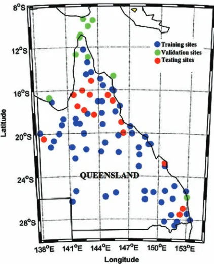
For the construction of the ANN and GP model, the data was partitioned into three sets of training, validation, and testing, comprising 60 Queensland cities for training, 10 Queensland cities for validation and 15 Queensland cities for model testing. Figure 4 shows the map of Queensland with training, testing and validation sites, Table 2 illustrates the data segregation for the modelling purpose. Furthermore, all predictors as well as objective variables were normalized using a normalization method. Normalization

Optimization of Windspeed Predictionl

can be performed between 0 and 1 or -1 and 1. The normalization gives equal weight to all variables (Afram, Janabi-Sharifi, Fung, & Raahemifar, 2017); it was done to reduce the time of learning because of large fluctuations in data and to ensure that the predictor variables do not affect the process of model construction. The data were normalized between 0 and 1 according to the following Equation .

X X X X X

norm =

− −

min

max min

where, X_norm,X_max and X_min represent the normalized, minimum, and maximum values of the variable

X, respectively.

3.2 Feature Selection

To achieve a high forecasting accuracy an optimal selection of input variables is vital. This is because there are often some features in the training datasets that might not be relevant to the leaning task. Some might even be noisy and have a negative impact on the performance of the forecasting model. In general, the impact of the input variables can be found in different ways by considering their relevance, computational effort, training difficulty, dimensionality and comprehensibility (May, Dandy, & Maier, 2011). The optimal input variable set will contain the fewest predictive variables required to describe the

Optimization of Windspeed Predictionl

behavior of the objective variable, Ws with a minimum degree of redundancy and with no uninformative (noise) variables. Kim (Kim, 2015) explains that the identification of an optimal set of input variables will lead to a more accurate, efficient, cost-effective and more easily interpretable ML model. Hence, it is vital to take advantage of feature selection algorithms that can identify the features that are relevant and necessary for the learning problem. In our modelling, we started with 10 different inputs (Table 1) downloaded as predictor variables and have done feature selection using neighborhood component analysis for regression (NCA). NCA is a non-parametric and embedded method for selecting features with the goal of maximizing prediction accuracy of regression algorithms (Yang, Wang, & Zuo, 2012). The MATLAB function called “fsrnca” performs NCA feature selection with regularization to learn feature weights for minimization of an objective function that measures the average ‘leave-one-out’ regression loss over the training data.

The fsrnca function performs NCA feature selection modified for regression. Given n observations

S ={( , ),x y i_{i i} =1 2, ,... },n

where x_{i ∈}p _{are the feature vectors, and y}

i = is a continuous function. The aim is to predict the

response y given the training set S.

Consider a randomized regression model that:

• Randomly picks a point (Re ( ))f x from S as the ‘reference point’ for x.

• The function sets the response value at x equal to the response value of the reference point

(Re ( ))f x

Again, the probability P Ref x( ( )=x S_j | ) that point x_j is picked from S as the reference point for x

is higher if x_j is closer to x as measured by the distance function d_w, where:

d x x_{w i j} w x_r x

r p

ir jr

( , )= −

=

∑

1

And w_r are the feature weights, assuming that,

P Ref x( ( )=x S_j )∝k d x x( (_w , _j)),

where, k is some kernel or a similarity function that assumes large values when d_w(x,x_j) is small. Sup-pose it is:

k z( )=exp−z ,   

   

σ

Optimization of Windspeed Predictionl

point for x is chosen from S, so the sum of P Ref x( ( )=x S_j | )for all j must be equal to 1. Therefore, it is possible to write:

P Ref x x S k d x x n d x x k

j

w j j

w j j N ( ( ) | ) ( ( )) ( ( )) , , = = =

∑

Now consider the ‘leave-one-out’ application of this randomized regression model that is predicting the response for x_i using the data in S−i_{, and the training set S excluding the point (x}

i, yi). The probability

that point x_j is picked as the reference point for x_i is:

p P Ref x x S k d x x d x x k

i j i j

w i j

w i j j j N = = − = = ≠

∑

Let yˆ_i be the response value the randomized regression model predicts and y_i be the actual response for x_i. Also let l :2 _{→ be a loss function that measures the disagreement between yˆ}

iand yi. Then,

the average value of l y y( _i, ˆ_i) is:

l_i =E_{( (}l y_{i, ˆ}y_{i) |}S−1₎= _{probability that is the reference pooint for}x_j

= , ( ) ( , ) , ,

x l y y

p l y y

i i j j j N ij j j N i j × = ≠ = ≠

∑

∑

After adding the regularization term, the objective function for minimization is:

f w

n li w

i n r r p ( )= + = =

∑

∑

Optimization of Windspeed Predictionl

After doing the feature selection using “fsrnca” a total of 7 input predictors were selected based on highest weights for all Queensland locations. The selected predictor variables after performing NCA feature selection are presented in Table 3.

3.3 Performance Evaluation

To evaluate the performance of ANN as well as the GP model, several statistical metrics were employed. The mathematical representations are enumerated as follows. Where, ws_OBS and ws_FOR are the observed and forecasted ith _{value of windspeed, wsOBS and wsFOR are the observed and forecasted mean windspeed}

and N is the number of datum points in the test set. 1. Correlation coefficient (r) expressed as:

r

ws ws ws ws

ws ws

OBS i OBS i FOR i FOR i i

N

OBS i OBS i

= −

(

)

(

)

(

)

∑

FOR i FOR i i N ws ws = =

∑

∑

(

)

The degree of collinearity between simulated and measured data ranges from −1 to 1 and is described by the correlation coefficient (r). If r = 0, no linear relationship exists. If r = 1 or −1, a perfect positive or negative linear relationship exists (Coimbra, Kleissl, & Marquez). The equation for r, however, is based on the consideration of a linear relationship between observed and simulated data.

2. Root mean square error (RMSE) is expressed as:

RMSE

N wsFOR i wsOBS i i N =

(

)

∑

1 , ,

The RMSE is a frequently used measure to compare forecasting errors of different models. In this case the RMSE of the target variable, Ws is expressed in ms-1_{. The lower RMSE value the better the}

predictive capability of a model in terms of its absolute deviation. However, presence of few large errors can result in a greater value of RMSE (Despotovic, Nedic, Despotovic, & Cvetanovic, 2016).

3. Mean absolute error (MAE) is expressed as:

MAE

N wsFOR i wsOBS i i N =

(

)

∑

Optimization of Windspeed Predictionl

Optimization of Windspeed Predictionl

The MAE is the sum of absolute values of the errors divided by the number of observations. This quantity is often used in statistics as a measure how close calculated values are to measured values (Willmott & Matsuura, 2005) .

4. Mean Bias error (MBE) is expressed as:

MBE ws ws N

FOR i OBS i

i n =

(

)

∑

This indicator expresses the tendency of forecast model to underestimate (negative value) or over-estimate (positive value) Ws. MBE values closest to zero are desirable. The drawback of this test is that it does not show the correct performance when the model presents overestimated and underestimated values at the same time, since overestimation and underestimation values cancel each other (Jiang, 2009). 5. Willmott’s Index (WI) is expressed as:

WI

ws ws

ws ws ws ws

FOR i OBS i i

N

FOR i OBS i OBS i OBS

= − −

(

)

∑

1 , ,

, , , ,ii

i N d

(

)

∑

The index of agreement (Willmott Index; WI) which signifies the ratio between the mean square error and the “potential error” was computed to overcome the issue with r, RMSE and MAE.

6. Relative root mean square error (RRMSE¸ %) is expressed as:

Table 3. Predictor variables used for modeling after feature selection

S.N Predictor Variable Unit

1 Latitude Deg

2 Air temperature Deg C

3 Atmospheric pressure kPa

4 Relative humidity %

5 Daily solar radiation - horizontal kWh/m2_/d

6 Earth temperature Deg C

Optimization of Windspeed Predictionl

RRMSE N

ws ws

N ws

FOR i OBS i i N OBS i i N = −

(

)

(

)

∑

∑

RRMSE is calculated by dividing RMSE with the average value of the measured observational data. A model’s precision level is excellent if the RRMSE < 10%, good if 10% < RRMSE < 20%, fair if 20% < RRMSE < 30% and poor if the RRMSE > 30% (Dawson, Abrahart, & See, 2007; Ravinesh C. Deo & Şahin, 2017; Jamieson, Porter, & Wilson, 1991; Moriasi, Arnold, Van Liew, Bingner, Harmel, & Veith, 2007; Shamshirband, Mohammadi, Chen, Narayana Samy, Petković, & Ma, 2015).

7. Relative root Mean absolute error (RMAE), is expressed as:

RMAE N

ws ws ws

FOR i OBS i

OBS i i N =

(

)

∑

The RMAE when expressed as a percentage is also known as mean absolute percentage error (MAPE) (Yadav & Chandel, 2014). This indicator is expressed as the average absolute value of relative differences between estimated and measured windspeed.

8. Nash–Sutcliffe coefficient (ENS), is expressed as:

E

ws ws

ws ws

NS

OBS i FORi i

N

OBS i OBS i i N = − − −           = =

∑

∑

, 0 E_NS 1

E_NS is a normalized statistic that governs the relative extent of the residual variance (“noise”) compared to the measured data variance (“information”) and provides a better assessment of a model as it is sensi-tive to differences in the observed and forecasted means and variances (Govindaraju, 2000).The closer the E_NS coefficient is to 1, the better the model’s performance (Qiaofeng, Xu, Siyu, & Xiaohui, 2015). 9. Legates and McCabe Index (E1), is expressed as:

E

ws ws

E

OBS i i i N FOR 1 1 1 0 = − −           ≤ =

∑

Optimization of Windspeed Predictionl

Legates and McCabe (1999) suggested a modified index of agreement (E₁) that is less sensitive to high extreme values because errors and differences are given appropriate weighting by using the absolute value of the difference instead of using the squared differences (Legates & McCabe, 1999).

10. Expanded uncertainty (U₉₅) expressed as:

U_{95 =1 96. (SD}2_+RMSE2 1 2₎/

Following Gueymard (Gueymard, 2014) and Behar et al.(Behar, Khellaf, & Mohammedi, 2015), this indicator is used in order to show more information about the model deviation. Where, 1.96 is the coverage factor corresponding to the 95% confidence level, and SD is the standard deviation of the dif-ference between the calculated and measured data.

11. t-statistic (t-stat) expressed as:

t stat N MBE RMSE MBE

- = −

−

( 1) 2

2 2

This indicator, which has had a long history of popular usage, was first proposed by Stone (Stone, 1993) to be used in combination with RMSE and MBE for more complete evaluation of models. For this research, t-statistics were used to validate whether the calculated values of windspeed are not significantly different from the measured observations. Better models have values closer to zero.

12. Global Performance Indicator (GPI) expressed as: GPI =MBE RMSE U× × ₉₅×t_stat× −₍₁ R2₎

The GPI is a multiplication of five statistical factors. These factors are less than unity. Therefore, the smaller the five statistics the smaller the GPI. The GPI combines the advantages of all the above-men-tioned indicators because it examines the short and long term performance and linearity of the models. It can be used for ranking the models since it offers a higher resolution as its values are in the order of 10−5_{. The first ranking model offers higher performance, with the highest modeling quality. The more}

the accuracy of the model, the closer to zero is the GPI (Stone, 1993).

3.4 ANN Implementation

Optimization of Windspeed Predictionl

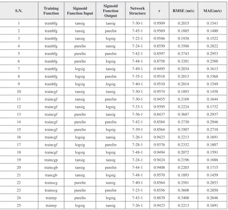
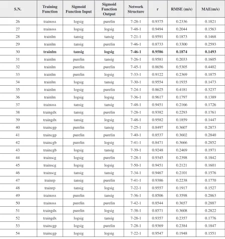
of 15–50 neurons were successively trialled until the output converged to a minimum Mean Square Error (MSE). In order to construct the best ANN model, the set of six back propagation training algo-rithms used were as follows: trainlm, trainscg, traincgp, traincgf, trainoss and trainbfg. Additionally, combinations of the input, hidden layer and output neurons of Equation [3] were tried one by one which resulted in a total of 54 ANN models being tested with different combinations of the transfer function (linear, hyperbolic-tangent sigmoid & log-sigmoid) for the hidden and output layer. As an additional measure, the correlation coefficient (r), RMSE and MAE of each trained model was noted to verify the model as detailed in Table 4. The ANN model with the Levenberg–Marquardt (LM) training function with tansig as sigmoid function for the input layer and logsig as sigmoid function for the output layer performed the best.

Table 4. Design parameters of artificial neural network (ANN) models with most appropriate 7 predictors, measured by correlation coefficient (r), root mean square error (RMSE) and mean absolute error (MAE).

S.N. _FunctionTraining _{Function Input}Sigmoid Function Sigmoid Output

Network

Structure r RMSE (m/s) MAE(m/s)

Optimization of Windspeed Predictionl

3.5 GP Implementation

A total of 17 runs were performed with varying population sizes (50-50000) and parameter settings as shown in Table 5. The best GP model was selected for each location based on minimum RMSE on validation data. The performance of each best GP model was evaluated on training, validation and test-ing data. Table 6 shows the performance of the devloped GP model. The GP model yielded the best

S.N. FunctionTraining Function InputSigmoid Function Sigmoid Output

Network

Structure r RMSE (m/s) MAE(m/s)

26 trainoss logsig purelin 7-28-1 0.9375 0.2336 0.1821 27 trainoss logsig logsig 7-48-1 0.9494 0.2044 0.1563 28 trainlm tansig tansig 7-21-1 0.9591 0.1873 0.1468 29 trainlm tansig purelin 7-46-1 0.8733 0.3300 0.2593

30 trainlm tansig logsig 7-46-1 0.9586 0.1874 0.1493

31 trainlm purelin tansig 7-26-1 0.9581 0.2033 0.1605 32 trainlm purelin purelin 7-45-1 0.8656 0.5305 0.4402 33 trainlm purelin logsig 7-33-1 0.9122 0.2369 0.1875 34 trainlm logsig tansig 7-30-1 0.9554 0.1935 0.1473 35 trainlm logsig purelin 7-24-1 0.8625 0.4181 0.3237 36 trainlm logsig logsig 7-36-1 0.9617 0.1797 0.1389 37 trainoss tansig tansig 7-48-1 0.9451 0.2166 0.1726 38 traingdx tansig purelin 7-28-1 0.9382 0.2293 0.1761 39 traingdx tansig logsig 7-48-1 0.9582 0.1859 0.1447 40 traincgp purelin tansig 7-25-1 0.8497 0.3607 0.2873 41 traincgp purelin purelin 7-40-1 0.8537 0.3602 0.2840 42 traincgb purelin logsig 7-41-1 0.8471 0.3666 0.2852 43 traincgb logsig tansig 7-39-1 0.9248 0.2469 0.1971 44 trainscg logsig purelin 7-28-1 0.9345 0.2398 0.1842 45 trainscg logsig logsig 7-50-1 0.9451 0.2121 0.1601 46 trainscg tansig tansig 7-34-1 0.9467 0.2101 0.1576 47 trainrp tansig purelin 7-41-1 0.9386 0.2238 0.1770 48 trainrp tansig logsig 7-22-1 0.9557 0.1917 0.1527 49 trainoss purelin tansig 7-36-1 0.8506 0.3598 0.2863 50 trainoss purelin purelin 7-42-1 0.8544 0.3657 0.2887 51 traingdx purelin logsig 7-38-1 0.8571 0.3608 0.2822 52 traingdx logsig tansig 7-28-1 0.9357 0.2357 0.1776 53 traincgp logsig purelin 7-28-1 0.9369 0.2384 0.1847 54 traincgp logsig logsig 7-22-1 0.9547 0.1948 0.1551

Optimization of Windspeed Predictionl

results with a population size of 10,000. Equation [38] shows the MGGP model for the best GP model (Abbreviation used as per Table 1).

Model =_{0 145.} P_atm−_{3 46.} e lat−5 −_{4 8.} e I−6 _rad+_{2 57.} e lat−5 −_{3 25.} e−5_*

eexp− . . exp . . tanh

  



 

− − −

(

)

(

)

0 263 1 0 0 33

T

long RH

air _EE

I lat e

temp

rad

(

)

+_{0 0136. exp(}−_{1 0. exp(}−_{1 0. * )1 2/ )}+_{0 64.} +_{4 12.} −7_{ttanh exp . *}

tanh . .

( ( ) )(

−

− − + +

(

)

(

)

1 57 1 0

P

long T

lat E

atm air

temp −−3 72. )+0 324.

4. RESULTS AND DISCUSSION

The measured and predicted values of Ws are plotted in Figure 5, it is clear that the predicted values are strongly correlated with the measured Ws data for the ANN model, with r ≈ 0.9545. ANN outper-forms the GP model, with the correlation coeffecient of the GP model being r ≈ 0.8314. Similarly, the analysis of RMSE and MAE of the ANN models provide positive evidence that the ANN is better than GP. Table 4 and 6 demonstrate the comparisons of evaluation parameters for the predictive performance of ANN and GP. In this case, RMSE (≈ 0.177 -0.5305 ms-1_{) and MAE (≈ 0.139- 0.44 ms}-1_{) were low}

for the ANN when compared to GP with RMSE (≈ 0.402-0.423 ms-1_{) and MAE (≈ 0.302 -0.356 ms}-1_).

The error histogram shows the variation of the error with instances. Figure 6 provides the authentica-tion to the ANN model with the major part of the data coinciding with the zero error line when compared with GP. To have a better understanding of the model accuracy for practical applications, the frequency of the error encountered was determined in various error brackets. A histogram of the frequency of

Table 5. Parameter settings for the genetic programming (GP) model

Run Parameters Value

Population size 50-50000

Number of generations 150

Number of runs 10

Parallel mode off

Tournament size 80

Elite fraction 0.7

Fitness cache enabled

Optimization of Windspeed Predictionl

Figure 5. Regression plot of the ANN and GP (Note: The line in blue and red is the least-squares fit line to the respective scatter plots, r is correlation coefficient).

Table 6. Design parameters of genetic programming (GP) models with most appropriate 7 predictors, measured by correlation coefficient (r), root mean square error (RMSE) and mean absolute error (MAE).

Population r RMSE (m/s) MAE(m/s)

50 0.8030 0.4123 0.3429

200 0.7954 0.4194 0.3555

500 0.7953 0.4157 0.3237

800 0.8046 0.4024 0.3130

1000 0.8072 0.4065 0.3301

1500 0.8101 0.4243 0.3523

2000 0.8107 0.4037 0.3292

4000 0.8122 0.3946 0.3231

5000 0.8236 0.3950 0.3134

8000 0.8187 0.3919 0.3102

10000 0.8314 0.3851 0.3016

15000 0.7813 0.4208 0.3397

20000 0.7806 0.4202 0.3387

25000 0.8028 0.4039 0.3220

30000 0.8065 0.4080 0.3319

40000 0.7755 0.4207 0.3340

Optimization of Windspeed Predictionl

forecasted error (FE) with a ±0.1 ms-1_day-1 _{error bracket has been prepared (Figure 7) Consistent with}

earlier results, the most correct forecasting is given by the ANN model. Remarkably, about 36% of the FE were seen to lie within the ± 0.1 ms-1_{error range for ANN (Figure 5) whereas for the GP (Figure 8),}

the recorded FE was about 20% of all errors within ± 0.1 ms-1_{. With ± 0.2 ms}-1_{ANN was also shown to}

be the better performing model with 71% of the FE falling within this error bracket.

The model assessment was also done using the normalized RMSE, RMAE and E₁ where the respec-tive percentages are used. In agreement with previous findings, the ANN model outperformed the GP model. The graph of predictor metrics versus the model under study are shown in Fig. 9. The relative RMSE, RMAE, E_NS and E₁ are higher for the ANN model, indicating better performance. Other metrics in the same figure further indicate the better performance of ANN compared to GP, with the lowest GPI (≈ 0), t-stat (≈ 0.842), MBE (≈ 0.011) and U₉₅ (≈ 0.519). Table 7 shows the measured and predicted values of Ws for the Queensland locations under study.

5. CONCLUSION

Optimization of Windspeed Predictionl

Figure 7. Cumulative frequency of daily forecasting errors of Ws (m/s) for ANN model when all testing locations are pooled together, X-axis showing the forecasted error of Ws (ms-1_).

Optimization of Windspeed Predictionl

Figure 9. Predictor metrices comparison for the best ANN and GP model.

Table 7. Predicted Values of Windspeed using ANN and GP models

Location Model Jan Feb March April May June July Aug Sept Oct Nov Dec

Optimization of Windspeed Predictionl

validation and 15 locations for testing. A total of eleven metrological data variables were extracted for the 85 locations from the publicly available NASA SSE6.0 dataset and optimised by the neighborhood component analysis (fsrnca) method of feature selection. In our study, we selected seven important predictor variables based on ‘fsrnca” which were: Latitude, Air temperature, Atmospheric Pressure, Relative Humidity, Daily Solar Radiation, Earth Temperature and Longitude.

Location Model Jan Feb March April May June July Aug Sept Oct Nov Dec

Paddys Green

Meas 4.50 4.80 5.50 5.90 5.70 5.30 5.50 5.40 5.80 5.40 5.10 4.90 ANN 4.63 4.71 5.27 5.79 5.79 5.26 5.25 5.56 5.75 5.55 5.15 4.78 GP 5.08 5.10 5.12 5.24 5.32 5.08 5.09 5.24 5.35 5.23 5.14 5.14 Karron Meas_ANN 4.50_4.68 4.60_4.73 5.10_5.33 5.30_{5.36 5.14}5.20 _4.694.80 _4.885.00 _5.094.90 _5.305.30 _5.295.00 4.90 4.70_{5.03 4.68} GP 4.81 4.83 4.85 4.86 4.88 5.03 4.86 4.95 4.84 4.77 4.79 4.81 Strathmore Meas_ANN 4.50_4.38 4.60_4.50 5.20_5.01 5.50_{5.25 5.11}5.30 _4.774.80 _4.845.00 _5.105.10 _5.185.60 _5.125.20 5.00 4.80_{4.86 4.55} GP 4.85 4.83 4.85 4.85 4.94 4.89 4.91 5.00 4.83 4.76 4.80 4.78 Georgetown _ANNMeas 4.50_4.40 4.50_4.39 5.10_4.87 5.20_5.19 5.00_{4.97 4.38}4.40 _4.424.80 _4.684.80 5.30_{5.15 5.17}5.10 4.90 4.70_{4.82 4.45} GP 4.84 4.91 4.90 4.97 4.96 4.64 4.63 4.78 4.97 4.87 4.85 4.85 Paluma Meas_ANN 4.50_4.37 4.30_4.47 5.10_4.97 5.20_{5.21 4.78}4.90 _4.153.80 _4.204.70 _4.594.70 _5.155.10 _5.255.00 5.00 4.50_{4.81 4.53} GP 4.89 4.91 4.92 5.02 5.00 4.67 4.63 4.80 5.10 4.98 4.93 4.88 Sellheim Meas_ANN 4.50_4.34 4.00_4.26 4.80_4.70 4.70_{4.69 4.29}4.40 _3.873.20 _3.974.20 _4.224.30 _4.824.80 _4.954.80 4.80 4.40_{4.74 4.42} GP 4.71 4.79 4.78 4.92 4.74 4.38 4.34 4.48 4.97 4.81 4.79 4.75 Barkly Meas_ANN 3.90_3.96 3.90_3.95 4.10_4.13 4.10_{4.10 4.10}4.30 _3.904.00 _4.054.10 _3.944.10 _4.164.40 _4.294.20 4.10 4.00_{4.03 3.99} GP 4.33 4.34 4.33 4.40 4.33 4.00 3.95 4.15 4.45 4.32 4.28 4.31 Weerriba Meas_ANN 4.50_4.67 4.70_4.89 5.00_5.22 4.90_{5.32 5.01}4.70 _4.654.50 _4.664.60 _4.654.50 _4.824.80 _4.984.60 4.70 4.40_{4.85 4.67} GP 4.59 4.59 4.61 4.71 4.83 4.36 4.37 4.53 4.83 4.70 4.62 4.61 Glenfern Meas_ANN 4.20_4.08 4.20_4.11 3.80_4.06 3.50_{3.92 3.79}3.50 _3.653.40 _3.673.60 _3.793.60 _4.093.80 _4.194.30 4.40 4.00_{4.12 4.07} GP 4.27 4.31 4.42 4.41 3.89 3.62 3.61 3.62 3.91 4.19 4.42 4.31 Adare Meas_ANN 3.50_3.82 3.60_3.79 3.70_3.70 3.70_{3.59 3.51}3.60 _3.523.60 _3.633.80 _3.543.70 _3.743.60 _3.873.70 3.90 3.60_{3.88 3.83} GP 4.31 4.30 4.40 4.31 3.66 3.56 3.60 3.52 3.70 3.96 4.15 4.31 *Note:- Meas:- is measured windspeed in m/s /day

Optimization of Windspeed Predictionl

A vast number of training algorithms and hidden transfer functions have been trailed in this study to achieve a prominent level of accuracy for the ANN model. The Levenberg–Marquardt backpropaga-tion (trainlm) algorithm with tangent sigmoid functions for hidden neuron and logarithmic sigmoid as transfer function for the output was adopted for the best prediction of Ws. Further, the ANN model was compared with GP models. The iteration was done on the number of population sizes for the GP model. The enumeration of major findings and results showed:

1. The better performance of ANN model was evidenced in terms of high correlation coefficient r

≈0.9686, low root mean square error, RMSE≈0.188 ms-1 _{and low mean absolute error MAE≈0.149}

ms-1_{, compared to low r ≈0.8314, high RMSE≈0.3851 ms}-1 _{and high MAE≈0.306 ms}-1 _{for the}

optimal GP model.

2. In terms of normalized performance metrics, Willmott index WI and Nash-Sutcliffe coefficient E_NS attained by the optimal ANN was higher than the GP model. The values of these metrics were WI≈0.961(ANN) and 0.647 (GP) and E_NS≈0.916 (ANN), and 0.648 (GP) respectively. The Mean bias error for ANN was ≈ 0.0118 ms-1 _{compared to 0.0328 ms}-1 _{for GP.}

3. By assessing the performance of ANN in relation to GP using the most advanced normalized metrics of LegatesMcCabes (LM), the ANN again outperformed the optimal GP model. The obtained LM agreement values between the predicted Ws and observed Ws were LM≈0.718 (ANN) and 0.430 (GP) respectively whereas the relative percentage errors RRMSE and RMAE ware only 3.89%, 3.19% (ANN) compared with 8.0%, 6.36% (GP).

4. In terms of expanded uncertainty U₉₅ ≈ 0.52, t-statistics (t-stat) ≈ 0.842 and global performance indicator GPI ≈ 4*10-5_{, the ANN model outperformed the GP model.}

Concisely, this study advocates the possibility of using publicly available climate data with suitable feature selection methods to predict the windspeed Ws. Such a technique has useful application for re-newable energy production and may be suited for selecting the best sites for development of wind power generators in the near future. The ANN model developed in this research can be optimized and tuned with other advanced techniques such as ensemble methods, particle swarm optimization PSO, genetic algorithms, fuzzy logic and so on. This study provides baseline information on the relevance of ANN at predicting local climatic factors., Other models such as support vector machine SVM and Extreme machine learning ELM which are built on and extend the commonly used ANN models may be utilized in future research to assess their potential for predicting windspeed in an Australian climate.

REFERENCES

Optimization of Windspeed Predictionl

Afram, A., Janabi-Sharifi, F., Fung, A. S., & Raahemifar, K. (2017). Artificial neural network (ANN) based model predictive control (MPC) and optimization of HVAC systems: A state of the art review and case study of a residential HVAC system. Energy and Building, 141, 96–113. doi:10.1016/j.en-build.2017.02.012

Alexiadis, M. C., Dokopoulos, P. S., Sahsamanoglou, H. S., & Manousaridis, I. M. (1998). Short-term forecasting of wind speed and related electrical power. Solar Energy, 63(1), 61–68. doi:10.1016/S0038-092X(98)00032-2

Amirkhani, S., Nasirivatan, S., Kasaeian, A. B., & Hajinezhad, A. (2015). ANN and ANFIS models to predict the performance of solar chimney power plants. Renewable Energy, 83, 597–607. doi:10.1016/j. renene.2015.04.072

Behar, O., Khellaf, A., & Mohammedi, K. (2015). Comparison of solar radiation models and their vali-dation under Algerian climate – The case of direct irradiance. Energy Conversion and Management, 98, 236–251. doi:10.1016/j.enconman.2015.03.067

Benth, J. Š., & Benth, F. E. (2010). Analysis and modelling of wind speed in New York. Journal of Ap-plied Statistics, 37(6), 893–909. doi:10.1080/02664760902914490

Bilgili, M., & Sahin, B. (2013). Wind speed prediction of target station from reference stations data.

Energy Sources. Part A, Recovery, Utilization, and Environmental Effects, 35(5), 455–466. doi:10.108 0/15567036.2010.512906

Blonbou, R. (2011). Very short-term wind power forecasting with neural networks and adaptive Bayesian learning. Renewable Energy, 36(3), 1118–1124. doi:10.1016/j.renene.2010.08.026

Cadenas, E., & Rivera, W. (2007). Wind speed forecasting in the south coast of Oaxaca, Mexico. Renew-able Energy, 32(12), 2116–2128. doi:10.1016/j.renene.2006.10.005

Cadenas, E., & Rivera, W. (2010). Wind speed forecasting in three different regions of Mexico, using a hybrid ARIMA–ANN model. Renewable Energy, 35(12), 2732–2738. doi:10.1016/j.renene.2010.04.022 Dawson, C. W., Abrahart, R. J., & See, L. M. (2007). HydroTest: A web-based toolbox of evaluation metrics for the standardised assessment of hydrological forecasts. Environmental Modelling & Software,

22(7), 1034–1052. doi:10.1016/j.envsoft.2006.06.008

Dee, D. P., Uppala, S. M., Simmons, A. J., Berrisford, P., Poli, P., Kobayashi, S., ... Vitart, F. (2011). The ERA-Interim reanalysis: Configuration and performance of the data assimilation system. Quarterly Journal of the Royal Meteorological Society, 137(656), 553–597. doi:10.1002/qj.828

Deo, R. C., & Sahin, M. (2017). Forecasting long-term global solar radiation with an ANN algorithm coupled with satellite-derived (MODIS) land surface temperature (LST) for regional locations in Queensland. Renewable & Sustainable Energy Reviews, 72, 828–848. doi:10.1016/j.rser.2017.01.114 Despotovic, M., Nedic, V., Despotovic, D., & Cvetanovic, S. (2016). Evaluation of empirical models for predicting monthly mean horizontal diffuse solar radiation. Renewable & Sustainable Energy Reviews,

Optimization of Windspeed Predictionl

Elbayoumi, M., Ramli, N. A., & Fitri Md Yusof, N. F. (2015). Development and comparison of re-gression models and feedforward backpropagation neural network models to predict seasonal indoor PM2.5–10 and PM2.5 concentrations in naturally ventilated schools. Atmospheric Pollution Research,

6(6), 1013–1023. doi:10.1016/j.apr.2015.09.001

Fan, G.-f., Wang, W.-s., & Liu, C. (2008). Wind power prediction based on artificial neural network.

Proceedings of the CSEE, 34, 118-123.

Farshad, F. F., Garber, J. D., & Lorde, J. N. (2000). Predicting temperature profiles in producing oil wells using artificial neural networks. Engineering Computations, 17(6), 735–754. doi:10.1108/02644400010340651 Fletcher, R., & Reeves, C. M. (1964). Function minimization by conjugate gradients. The Computer Journal, 7(2), 149–154. doi:10.1093/comjnl/7.2.149

Foley, A. M., Leahy, P. G., Marvuglia, A., & McKeogh, E. J. (2012). Current methods and advances in forecasting of wind power generation. Renewable Energy, 37(1), 1–8. doi:10.1016/j.renene.2011.05.033 Garg, A., Vijayaraghavan, V., Mahapatra, S. S., Tai, K., & Wong, C. H. (2014). Performance evalua-tion of microbial fuel cell by artificial intelligence methods. Expert Systems with Applications, 41(4), 1389–1399. doi:10.1016/j.eswa.2013.08.038

Gharbi, R., & Elsharkawy, A. (1996). Neural-network model for estimating the PVT properties of Middle East crude oils. In Situ, 20(4), 367–394.

Gharbi, R., & Elsharkawy, A. M. (1997). Neural network model for estimating the PVT properties of Middle East crude oils. Paper presented at the Middle East Oil Show and Conference. 10.2118/37695-MS Ghorbani, M., Khatibi, R., Hosseini, B., & Bilgili, M. (2013). Relative importance of parameters affecting wind speed prediction using artificial neural networks. Theoretical and Applied Climatology, 114(1-2), 107–114. doi:10.100700704-012-0821-9

Govindaraju, R. S. (2000). Artificial neural networks in hydrology. II: Hydrologic applications. Journal of Hydrologic Engineering, 5(2), 124–137. doi:10.1061/(ASCE)1084-0699(2000)5:2(124)

Gueymard, C. A. (2014). A review of validation methodologies and statistical performance indicators for modeled solar radiation data: Towards a better bankability of solar projects. Renewable & Sustainable Energy Reviews, 39, 1024–1034. doi:10.1016/j.rser.2014.07.117

Hagan, M. T., Demuth, H. B., & Beale, M. H. (1996). Neural network design. PWS Pub. Co.

Hinchliffe, M., Hiden, H., McKay, B., Willis, M., Tham, M., & Barton, G. (1996). Modelling chemical process systems using a multi-gene. Late Breaking Papers at the Genetic Programming, 56-65.

Optimization of Windspeed Predictionl

Kamble, L. V., Pangavhane, D. R., & Singh, T. P. (2015). Neural network optimization by comparing the performances of the training functions -Prediction of heat transfer from horizontal tube immersed in gas–solid fluidized bed. International Journal of Heat and Mass Transfer, 83, 337–344. doi:10.1016/j. ijheatmasstransfer.2014.11.085

Kariniotakis, G., Stavrakakis, G., & Nogaret, E. (1996). Wind power forecasting using advanced neural networks models. IEEE Transactions on Energy Conversion, 11(4), 762–767. doi:10.1109/60.556376 Kim, M. K. (2015). Short-term price forecasting of Nordic power market by combination Levenberg&#x2013;Marquardt and Cuckoo search algorithms. IET Generation, Transmission & Dis-tribution, 9(13), 1553–1563. doi:10.1049/iet-gtd.2014.0957

Kobayashi, S., Ota, Y., Harada, Y., Ebita, A., Moriya, M., Onoda, H., ... Takahashi, K. (2015). The JRA-55 Reanalysis: General Specifications and Basic Characteristics. Journal of the Meteorological Society of Japan.Ser. II, 93(1), 5–48. doi:10.2151/jmsj.2015-001

Koza, J. R. (1994). Genetic Programming II Videotape: The Next Generation (Vol. 55). MIT Press Cambridge.

Kriesel, D. (2007). A brief Introduction on Neural Networks. Academic Press.

Legates, D. R., & McCabe, G. J. Jr. (1999). Evaluating the use of “goodness‐of‐fit” measures in hydrologic and hydroclimatic model validation. Water Resources Research, 35(1), 233–241. doi:10.1029/1998WR900018 Makinde, F., Ako, C., Orodu, O., & Asuquo, I. (2012). Prediction of crude oil viscosity using feed-forward back-propagation neural network (FFBPNN). Petroleum and Coal, 54(2), 120–131.

Masrur, H., Nimol, M., Faisal, M., & Mostafa, S. M. G. (2016). Short term wind speed forecasting us-ing Artificial Neural Network: A case study. Paper presented at the 2016 International Conference on Innovations in Science, Engineering and Technology (ICISET). 10.1109/ICISET.2016.7856485 MathWorks. (1996). MATLAB: the language of technical computing: computation, visualization, pro-gramming: installation guide for UNIX version 5. Natwick: Math Works Inc.

May, R., Dandy, G., & Maier, H. (2011). Review of input variable selection methods for artificial neural networks. INTECH Open Access Publisher. doi:10.5772/16004

Mohandes, M. A., Rehman, S., & Halawani, T. O. (1998). A neural networks approach for wind speed prediction. Renewable Energy, 13(3), 345–354. doi:10.1016/S0960-1481(98)00001-9

Møller, M. F. (1993). A scaled conjugate gradient algorithm for fast supervised learning. Neural Net-works, 6(4), 525–533. doi:10.1016/S0893-6080(05)80056-5

Moriasi, D. N., Arnold, J. G., Van Liew, M. W., Bingner, R. L., Harmel, R. D., & Veith, T. L. (2007). Model evaluation guidelines for systematic quantification of accuracy in watershed simulations. Trans-actions of the ASABE, 50(3), 885–900. doi:10.13031/2013.23153

Optimization of Windspeed Predictionl

Pham, D. T., & Sagiroglu, S. (2001). Training multilayered perceptrons for pattern recognition: A comparative study of four training algorithms. International Journal of Machine Tools & Manufacture,

41(3), 419–430. doi:10.1016/S0890-6955(00)00073-0

Poli, R., Langdon, W., & McPhee, N. (2008). A field guide to genetic programming. Retrieved from http://lulu. com.

Qiaofeng, T., Xu, W., Siyu, C., & Xiaohui, L. (2015). Daily runoff time-series prediction based on the adaptive neural fuzzy inference system. Paper presented at the 2015 12th International Conference on Fuzzy Systems and Knowledge Discovery (FSKD).

Quej, V. H., Almorox, J., Arnaldo, J. A., & Saito, L. (2017). ANFIS, SVM and ANN soft-computing techniques to estimate daily global solar radiation in a warm sub-humid environment. Journal of Atmo-spheric and Solar-Terrestrial Physics, 155, 62–70. doi:10.1016/j.jastp.2017.02.002

Rahdari, F., Eftekhari, M., & Mousavi, R. (2016). A two-level multi-gene genetic programming model for speech quality prediction in Voice over Internet Protocol systems. Computers & Electrical Engineer-ing, 49, 9–24. doi:10.1016/j.compeleceng.2015.10.008

Raja, M. A. (2008). Real-time non-intrusive speech quality estimation of voice over internet protocol using genetic programming (PhD thesis). Electronic and Computer Engineering, University of Limerick, Ireland.

Rienecker, M. M., Suarez, M. J., Gelaro, R., Todling, R., Bacmeister, J., Liu, E., ... Kim, G.-K. (2011). MERRA: NASA’s modern-era retrospective analysis for research and applications. Journal of Climate,

24(14), 3624–3648. doi:10.1175/JCLI-D-11-00015.1

Searson, D. P., Leahy, D. E., & Willis, M. J. (2010). GPTIPS: an open source genetic programming toolbox for multigene symbolic regression. Proceedings of the International multiconference of engineers and computer scientists.

Seo, K., & Hyeon, B. (2015). Evolutionary nonlinear Model Output Statistics for wind speed predic-tion using Genetic Programming. Paper presented at the 2015 7th International Joint Conference on Computational Intelligence (IJCCI).

Shamshirband, S., Mohammadi, K., Chen, H.-L., Narayana Samy, G., Petković, D., & Ma, C. (2015). Daily global solar radiation prediction from air temperatures using kernel extreme learning machine: A case study for Iran. Journal of Atmospheric and Solar-Terrestrial Physics, 134, 109–117. doi:10.1016/j. jastp.2015.09.014

Sharma, B., & Venugopalan, K. (2014). Comparison of neural network training functions for hematoma classification in brain CT images. IOSR-JCE, 16(1), 31–35. doi:10.9790/0661-16123135

Admin-Optimization of Windspeed Predictionl

Stone, R. J. (1993). Improved statistical procedure for the evaluation of solar radiation estimation models.

Solar Energy, 51(4), 289–291. doi:10.1016/0038-092X(93)90124-7

Ul-Saufie, A. Z., Yahaya, A. S., Ramli, N. A., Rosaida, N., & Hamid, H. A. (2013). Future daily PM 10 concentrations prediction by combining regression models and feedforward backpropagation mod-els with principle component analysis (PCA). Atmospheric Environment, 77, 621–630. doi:10.1016/j. atmosenv.2013.05.017

Willmott, C. J., & Matsuura, K. (2005). Advantages of the mean absolute error (MAE) over the root mean square error (RMSE) in assessing average model performance. Climate Research, 30(1), 79–82. doi:10.3354/cr030079

Yadav, A. K., & Chandel, S. S. (2014). Solar radiation prediction using Artificial Neural Network tech-niques: A review. Renewable & Sustainable Energy Reviews, 33, 772–781. doi:10.1016/j.rser.2013.08.055 Yang, W., Wang, K., & Zuo, W. (2012). Neighborhood Component Feature Selection for High-Dimensional Data. JCP, 7(1), 161–168. doi:10.4304/jcp.7.1.161-168

Zameer, A., Arshad, J., Khan, A., & Raja, M. A. Z. (2017). Intelligent and robust prediction of short term wind power using genetic programming based ensemble of neural networks. Energy Conversion and Management, 134, 361–372. doi:10.1016/j.enconman.2016.12.032

Zhu, X., & Genton, M. G. (2012). Short‐Term Wind Speed Forecasting for Power System Operations.