Numerical solution of two-point boundary-value problems

NUMERICAL SOLUTION OF TWO-POINT

BOUNDARY-VALUE PROBLEMS

Thesis By

Andrew Benjamin White, Jr.

In Partial Fulfillment of the Requirements

For the Degree of

Doctor of Philosophy

California Institute of Technology

Pasadena, California 91109

1974

Acknowledgements

The a u t h o r w i s h e s t o t h a n k P r o f e s s o r H e r b e r t B , K e l l e r f o r h i s p a t i e n t guidence and i n v a l u a b l e a s s i s t a n c e i n t h e p r e p a r a t i o n of t h i s t h e s i s . H i s encouragement and e n t h u s i a s m were e s s e n t i a l t o t h e completion of t h i s work.

The o p p o r t u n i t y t o c a r r y o u t t h i s r e s e a r c h was p r o v i d e d by C a l i f o r n i a I n s t i t u t e of Technology Graduate Teaching A s s i s t a n t s h i p s f o r which t h e a u t h o r i s g r a t e f u l . H e a l s o w i s h e s t o e x p r e s s h i s a p p r e c i a t i o n t o t h e e n t i r e Department of Applied Mathematics, b o t h f a c u l t y and s t u d e n t s , f o r p r o v i d i n g a n i n v i g o r a t i n g c l i m a t e i n which t o p u r s u e t h i s work.

ABSTRACT

The a p p r o x i m a t i o n of two-point boundary-value problenls by g e n e r a l f i n i t e d i f f e r e n c e schemes i s t r e a t e d . A n e c e s s a r y and s u f f i c i e n t c o n d i t i o n f o r t h e s t a b i l i t y of t h e l i n e a r d i s c r e t e boundary-value problem i s d e r i v e d i n terms of t h e a s s o c i a t e d d i s c r e t e i n i t i a l - v a l u e problem. P a r a l l e l s h o o t i n g methods a r e shown t o b e e q u i v a l e n t t o t h e d i s c r e t e boundary-value problem. One-step d i f f e r e n c e schemes a r e c o n s i d e r e d i n d e t a i l and a c l a s s of c o m p u t a t i o n a l l y e f f i c i e n t schemes o f a r b i t r a r i l y h i g h o r d e r of a c c u r a c y i s e x h i b i t e d . S u f f i c i e n t c o n d i t i o n s a r e found t o i n s u r e t h e convergence of d i s c r e t e f i n i t e d i f f e r e n c e a p p r o x i m a t i o n s t o

n o n l i n e a r boundary-value problems w i t h i s o l a t e d s o l u t i o n s . ~ e w t o n ' s method

i s c o n s i d e r e d a s a p r o c e d u r e f o r s o l v i n g t h e r e s u l t i n g

Table of Contents

TITLE

PAGE

Introduction

Chapter 1. Linear Two-Point Boundary-Value

Problems

1. Existence Theory

2. Numerical Methods

3. Convergence for Linear Boundary-

Value Problems

Chapter 2. Difference Schemes

1. Taylor Series

2. Quadrature

3. Gap Schemes

4.

Other Schemes

5.

Stability of Triangular Schemes

6. Asymptotic Error Expansions

7. Increased Accuracy

Chapter 3. Parallel Shooting

1. Parallel Shooting

2. Method of Complementary Functions

3. Method of Adjoints

Chapter

4.

Nonlinear Two-Point Boundary-Value

Problems

1. Finite Difference Schemes

2. Existence of Solutions

3.

Newton's Method

4.

Equivalence of Shooting and Implicit

Schemes

Chapter 6 . A Numerical Example: P l a n e C o u e t t e Flow

1. I s o l a t e d S o l u t i o n

2 . Numerical P r o c e d u r e

3 . Numerical R e s u l t s Appendix A

I n t r o d u c t i o n

T h i s t h e s i s d e a l s w i t h t h e a p p l i c a t i o n of f i n i t e d i f f e r e n c e schemes t o two-point boundary-value problems. The assumption i s made throughout t h a t t h e s e boundary-value problems have i s o l a t e d s o l u t i o n s ; t h a t i s , t h e homogeneous, l i n e a r i z e d problem h a s o n l y t h e t r i v i a l s o l u t i o n , The g e n e r a l t h e o r y developed p l a c e s no r e s t r i c t i o n s on t h e form of t h e d i f f e r e n c e e q u a t i o n s ,

I n

r e p l a c e t h e boundary c o n d i t i o n s . From t h i s r e s u l t , i t i s c l e a r t h a t a s i m p l e s h o o t i n g method i s , i n f a c t ,

a

schemes.

In Chapter 3 , t h e e q u i v a l e n c e r e s u l t of Theorem 1.16 i s g e n e r a l - i z e d t o i n c l u d e a l l p a r a l l e l s h o o t i n g methods. Theorem 3 . 2 2 shows

t h a t t h e s e methods a r e e a c h a p a r t i c u l a r p r o c e d u r e f o r s o l v i n g t h e e q u a t i o n s d e r i v e d from approximating l i n e a r boundary-value problems. The Method of Complementary F u n c t i o n s i s examined i n d e t a i l a s a n example of methods f o r s o l v i n g problems w i t h s e p a r a t e d boundary

c o n d i t i o n s . The Method of A d j o i n t s i s a l s o c o n s i d e r e d and i t i s shown t h a t t h i s method i s n o t i n g e n e r a l e q u i v a l e n t t o t h e d i s c r e t e

boundary-value problem,

Nonlinear boundary-value problems a r e d e a l t w i t h i n Chapter 4. The d i f f e r e n c e schemes examined i n Chapter 2 a r e g e n e r a l i z e d t o be a p p l i c a b l e t o n o n l i n e a r d i f f e r e n t i a l e q u a t i o n s . Following Keller [

6

1,

Chapter 5 i s concerned w i t h t h e p r a c t i c a l problem of s o l v i n g t h e systems of a l g e b r a i c e q u a t i o n s a r i s i n g from t h e a p p r o x i m a t i o n of boundary-value problems w i t h s e p a r a t e d boundary c o n d i t i o n s . These e q u a t i o n s a r e w r i t t e n i n b l o c k t r i d i a g o n a l form, Mx = b. The s p e c i a l z e r o s t r u c t u r e of t h i s system i s e x p l o i t e d t o show t h a t , w i t h a n a p p r o p r i a t e row s w i t c h i n g s t r a t e g y , such a m a t r i x p o s s e s s e s a s i m p l e b l o c k LU decomposition i f and o n l y i f

M

A n u m e r i c a l example i s p r e s e n t e d i n Chapter 6. The e q u a t i o n s c o n s i d e r e d model p l a n e C o u e t t e flow. The Gap4 scheme, a s d e r i v e d i n Chapter

4 ,

n o n l i n e a r e q u a t i o n s .

Chapter I

L i n e a r Two-Point Boundary-Value Problems

1. E x i s t e n c e Theory

W e c o n s i d e r t h e system of n f i r s t - o r d e r , l i n e a r o r d i n a r y d i f f e r e n t i a l e q u a t i o n s :

where u ,

f,

6

0 1

p r o c e e d i n g t o t h e n u m e r i c a l approximation of ( l . l a , b ) , we p r e s e n t a n e x i s t e n c e and uniqueness r e s u l t c o n v e n i e n t f o r o u r p u r p o s e s .

Theorem 1 . 2 . L e t A ( t ) E c m [ o , l ] f o r some m 5 o. D e f i n e t h e fundamental m a t r i x ~ ( t ) a s t h e s o l u t i o n of

X' ( t )

-

Then f o r e a c h f ( t ) E c m [ o , l ] and

6

unique s o l u t i o n y ( t ) E

cm+l

,

.

P r o o f : The s o l u t i o n t o t h e i n i t i a l - v a l u e problem

Uniqueness f o r t h e i n i t i a l - v a l u e problem i n s u r e s t h a t X(t) i s n o n s i n g u l a r on [ o , l ] . The boundary-value problem ( l . l a , b ) h a s a s o l u t i o n i f and o n l y i f we c a n d e f i n e a n n-vector r such t h a t y ( t ) s a t i s f i e s t h e boundary c o n d i t i o n

T h i s r e q u i r e s

Thus, ( l . l a , b ) h a s a unique s o l u t i o n i f and o n l y i f [B

+

1

0 1

n o n s i n g u l a r . That y ( t ) E cm+'[o,l] i s an o b s e r v a t i o n from t h e form

of d i f f e r e n t i a l e q u a t i o n ( 1 . l a ) .

2 . Numerical Methods

Here w e d i s c u s s some s t a n d a r d c o n c e p t s of n u m e r i c a l a n a l y s i s and develop some n o t a t i o n . I n approximating t h e s o l u t i o n of

i = J

( l . l a , b ) , w e w i l l e m p l o y a n e t o f p o i n t s I t , } on [ o , l ] a n d a n e t i = J

f u n c t i o n {v,

1

Each v

i s a n n-vector and

where V i s a n n ( J + l ) - v e c t o r , W e d e f i n e t h e mesh w i d t h s max

hi = ti

-

i-1' o i'

t h a t f o r e a c h hi t h e r e e x i s t s a

A

>

i

T h i s c o n d i t i o n merely s t i p u l a t e s t h a t

E s min h./max hi 5 1

1

and t h u s t h e mesh becomes d e n s e i n [ o , l ] a s ho + o.

The norm we w i l l employ i s

1

I V

1 1

0 S i l J I l v i l l and f o r

b l o c k m a t r i c e s , t h e u s u a l induced norm max

l l ~ l l

I l v l l

I

IwI

1

I n t h e n = l c a s e , t h i s induced norm e q u a l s t h e maximum a b s o l u t e row sum, however t h i s r e s u l t does n o t g e n e r a l i z e t o n

>

max J

I I"I

I

'

osi<J

where M i s a n n x n m a t r i x element of t h e b l o c k m a t r i x M. i j

The boundary c o n d i t i o n s ( l . l b ) a r e approximated by

We d e f i n e t h e t r u n c a t i o n e r r o r T t o b e i

where y ( t ) i s any s o l u t i o n of t h e d i f f e r e n t i a l e q u a t i o n ( l o l a ) . S i m i l a r l y , we d e f i n e a t r u n c a t i o n e r r o r T a s s o c i a t e d w i t h t h e

0

boundary c o n d i t i o n s

where

y

.

ro w i l l always b e

the

More briefly, we will write

where

B

is an n(J+l)

n(J+l) matrix and r is an n(J+l)-vector

h

with ro =

Employing Euler's method to approximate the differential

equation (lala), this formulation of the discrete problem becomes

This example will be used throughout to illustrate various points of

interest.

Consistency. The difference approximation (1.5a) is said

to be consistent with the differential equation (l.la) iff

Thus, ~ u l e r ' s method i s c o n s i s t e n t and we s a y t h a t i t i s f i r s t - o r d e r a c c u r a t e because t h e l e a d i n g term i n t h e t r u n c a t i o n e r r o r expansion i s l i n e a r i n h

.

i

Order of a c c u r a c y . A n u m e r i c a l scheme h a s a n o r d e r of a c c u r a c y p

>

f o r a l l n e t s w i t h h o 5 H.

S t a b i l i t y . L e t V b e a s o l u t i o n t o (1.8). The d i f f e r e n c e scheme (1.8) i s s a i d t o b e s t a b l e i f f t h e r e e x i s t c o n s t a n t s

K 2 o, and H

>

0

f o r a l l n e t s w i t h

ho

>

f o r a l l n e t s w i t h ho 5 H.

Convergence. The n u m e r i c a l scheme (1.8) i s c o v e r g e n t iff max

o S i < J I l y ( t i )

-

h

.

A s t a n d a r d r e s u l t may now b e s t a t e d ,

Lemma 1.10 L e t t h e boundary-value problem ( l . l a , b ) have t h e e x a c t s o l u t i o n y ( t ) . L e t t h e d i s c r e t e boundary-value problem

b e c o n s i s t e n t w i t h ( l . l a , b ) and s t a b l e . Then t h e method i s c o n v e r g e n t , t h a t i s ,

P r o o f : The d e f i n i t i o n of t h e t r u n c a t i o n e r r o r ~ [ y ( t ) ] combined w i t h (1.5a, b ) g i v e s

By h y p o t h e s i s , t h e d i f f e r e n c e scheme i s s t a b l e , t h u s t h e r e e x i s t c o n s t a n t s KO 2 0 , H

>

Hence,

max

l

l y

-

'I l

I

-

1

For any p a r t i c u l a r scheme, we would l i k e t o be a b l e t o show t h a t t h e n e t f u n c t i o n approximates t h e e x a c t s o l u t i o n a t t h e n e t p o i n t s : t h a t t h e method i s c o n v e r g e n t . The t r u n c a t i o n e r r o r and o r d e r of a c c u r a c y a r e g e n e r a l l y d e r i v e d v i a T a y l o r ' s Theorem, a s was done i n t h e example of ~ u l e r ' s method. I n o r d e r t o show t h a t ~ u l e r ' s method i s convergent f o r t h e d i s c r e t e boundary-value problem, we need t o prove t h a t t h e m a t r i x

Bh

0

scheme would b e c o n v e r g e n t . However, even i n t h i s s i m p l e c a s e , t h e n o n s i n g u l a r i t y of

Bh

I n Theorem 1 . 2 t h e i n i t i a l - v a l u e problem i s used t o prove well-posedness of t h e boundary-value problem. A s K e l l e r

[ 5 ]

~ ( 0 ) =

B

S i m i l a r l y , we d e f i n e t h e d i s c r e t e i n i t i a l - v a l u e m a t r i x

Th

%

To form

I

i3

h'

1 , 0 r e s p e c t i v e l y .

3 . Convergence f o r l i n e a r boundary-value problems _--

T h e main r e s u l t of t h i s c h a p t e r i s t h a t a n u m e r i c a l scheme a p p l i e d t o a boundary-value problem w i t h a unique s o l u t i o n i s s t a b l e and c o n s i s t e n t i f and o n l y i f t h e a s s o c i a t e d i n i t i a l - v a l u e problem i s s t a b l e and c o n s i s t e n t . I t w i l l be u s e f u l t o prove s e v e r a l lemmas f i r s t .

Lemma 1.12 ( F a c t o r i z a t i o n ) Let

7

where L is a (J+l)n

n+l matrix

N is an (n+l)

(J+l)n matrix

and

6

is an (n+l)-vector

Proof: We take (1.7) to be the most general form of the boundary-value

matrix

Bh.

It may b e d i r e c t l y v e r i f i e d t h a t L,N,C a r e t h e p r o p e r f a c t o r s , b u t t h e sequence of o p e r a t i o n s below may c l a r i f y t h e d e r i v a t i o n .

The i d e n t i t y ro =

6

'

Lemma 1.13 (Reducing) L e t L,N be pxq and qxp m a t r i c e s r e s p e c t i v e l y . Let x and b be a p-vector and a q-vector r e s p e c t i v e l y . F u r t h e r , l e t L have r a n k q 5 p. Then t h e m a t r i x e q u a t i o n

h a s a s o l u t i o n

i f and o n l y i f

a r e l i n e a r l y i n d e p e n d e n t . T h e r e f o r e , t h e r e e x i s t s a p x ( P - ~ ) m a t r i x

L

W e may write any v e c t o r x E EP u n i q u e l y a s

Using t h i s r e p r e s e n t a t i o n i n (1.14),

The v e c t o r x i s a s o l u t i o n of (1.14) i f and o n l y i f

and

The n e c e s s i t y f o l l o w s .

m

Note t h a t t h i s lemma r e d u c e s t h e s o l u t i o n of p s i m u l t a n e o u s e q u a t i o n s

t o s o l u t i o n of q e q u a t i o n s , q 5 p ,

Theorem 1.16 L e t t h e boundary-value problem ( l , l a , b ) have a 1

unique s o l u t i o n y ( t ) E

c

a ) The d i s c r e t e boundary-value problem i s s t a b l e , c o n s i s t e n t (and c o n v e r g e n t ) .

b ) The a s s o c i a t e d i n i t i a l - v a l u e problem i s s t a b l e , c o n s i s t e n t (and c o n v e r g e n t ) .

P r o o f : (b

=>

The i n i t i a l - v a l u e problem i s s t a b l e by h y p o t h e s i s , t h e r e f o r e

Ih

ho

-1

Ih

D e f i n e Z and z by

where Z i s a n n ( J + l ) x n m a t r i x and z i s a n n ( ~ + l ) - v e c t o r , From ( 1 . 1 8 ) , we n o t e t h a t Z s a t i s f i e s

max

o r i l J

IIzi

-

0

and i n p a r t i c u l a r

I

IzJ

-

.

By v i r t u e of ( 1 , 1 8 ) , we may w r i t e (1.17) a s

v

+

-

51

.

1

The odumns of t h e n ( J + l ) x n + l m a t r i x [Z , z ] a r e l i n e a r l y independent s t

provided t h a t

r,

#

I

z e r o v e c t o r w e remove i t , r e p l a c e =

k ]

[e]

#

j

some j .

By t h e Reducing Lemma, (1.20) h a s a s o l u t i o n i f and o n l y i f

- 1

and t h e s o l u t i o n must be of t h e form

W e r e c a l l t h a t Zo = I and t a k e A = 1, s o t h a t (1.21) i s e q u i v a l e n t t o

s o l u t i o n of t h e boundary-value problem ( l . l a , b ) . E x i s t e n c e and u n i q u e n e s s of t h e s o l u t i o n , V, of t h e d i s c r e t e boundary-value

problem now h i n g e on t h e n o n - s i n g u l a r i t y of (B

+

0

By h y p o t h e s i s y ( t ) i s u n i q u e , and Theorem 1 . 2 s t a t e s t h a t

[Bo

+

t h u s , by t h e Banach Lemma, B

+

0 1 J

w i t h ho 5 H, provided H i s s o s m a l l t h a t f o r some

p

It i s c l e a r t h a t t h e d i s c r e t e boundary-value problem i s s t a b l e s i n c e

and Z and z a r e s o l u t i o n s of d i s c r e t e i n i t i a l - v a l u e problems, which were assumed s t a b l e .

( a

=>

I h V - r = o .

Following t h e F a c t o r i z a t i o n Lermna ( 1 . 1 2 ) , w e may w r i t e

Th

v

-

r

Bhv

-

L{NV

+

6 1 .

A

8 i s non-singular and we may d e f i n e [ Z

!

21

h

The Reducing Lemma (1.13) now i m p l i e s t h a t t h e s o l u t i o n V of (1.23) must be of t h e form

and e x i s t s i f and o n l y i f

A

T h e r e f o r e , w e wish t o show t h a t Z i s non-singular f o r a l l n e t s w i t h

0

h 5 H, f o r H s u f f i c i e n t l y s m a l l . Theorem 1 . 2 d e r i v e s t h e s o l u t i o n 0

of t h e boundary-value problem t o be

where r must s a t i s f y

Thus, t h e s o l u t i o n t o t h e boundary-value problem

A

2'

-

+

-

where R i s a n n x n m a t r i x and must s a t i s f y

By h y p o t h e s i s y ( t ) i s u n i q u e , t h u s t h e m a t r i x R i s n o n - s i n g u l a r ,

A A

t h a t i s , X(o) i s n o n - s i n g u l a r . W e n o t e t h a t Z a s d e f i n e d i n (1.24) i s a c o n v e r g e n t a p p r o x i m a t i o n t o t h e e q u a t i o n s ( 1 . 2 6 ) , hence

A

a n d , a s b e f o r e , Z i s n o n - s i n g u l a r f o r a l l n e t s w i t h h 5 H , where

0 0

H i s s u f f i c i e n t l y s m a l l . Now,

and t h e d i s c r e t e i n i t i a l - v a l u e problem h a s a s t a b l e s o l u t i o n .

m

W e r e c a l l t h a t t h e o r d e r of a c c u r a c y of a scheme i s d e t e r m i n e d by t h e l a r g e s t i n t e g e r p s u c h t h a t

I

1 1

0

C o r o l l a r y 1.27. L e t t h e boundary-value problem ( l . l a , b ) have a u n i q u e s o l u t i o n y ( t ) E C P + ~ [ O , ~ ] , f o r some i n t e g e r p 2 1. L e t t h e d i s c r e t e a p p r o x i m a t i o n s ( 1 . 5 a , b ) b e p-order a c c u r a t e , F u r t h e r , l e t t h e d i s c r e t e i n i t i a l - v a l u e problem a s s o c i a t e d w i t h ( 1 . 5 a , b ) b e s t a b l e . Then f o r a l l n e t s w i t h ho 5 H ,

i n d e p e n d e n t of h o e

P r o o f . The proof f o l l o w s t h a t of Theorem 1 . 1 6 .

These r e s u l t s and t h e m a n i p u l a t i o n s l e a d i n g t o them. s u g g e s t s e v e r a l f u r t h e r t o p i c s , Chapter 11 w i l l b e concerned w i t h t h e o p e r a t i o n a l c h a r a c t e r i s t i c s of v a r i o u s s p e c i f i c n u m e r i c a l schemes, Theorem 1.16 w i l l b e e x p l o i t e d t o d e t e r m i n e t h e s t a b i l i t y p r o p e r t i e s of a p a r t i c u l a r c l a s s of schemes. W e w i l l examine a s y m p t o t i c

e r r o r e x p a n s i o n s and d i s c u s s methods of i n c r e a s i n g t h e a c c u r a c y of d i s c r e t e a p p r o x i m a t i o n s . I n Chapter 111, we w i l l e n l a r g e upon Theorem 1.16 and t h e e q u i v a l e n c e of d i s c r e t e i n i t i a l - v a l u e and boundary-value problems.

D r . H , 0 , Kreiss h a s r e c e n t l y p u b l i s h e d a p a p e r

[ 7 ]

d e a l i n g w i t h t h e s t a b i l i t y of d i s c r e t e a p p r o x i m a t i o n s t o a r b i t r a r y o r d e r s y s t e m s of l i n e a r o r d i n a r y d i f f e r e n t i a l e q u a t i o n s . Thus, i t

Chapter I1

D i f f e r e n c e Schemes

I n t h i s c h a p t e r , w e w i l l examine some s p e c i f i c d i f f e r e n c e schemes; of p a r t i c u l a r i n t e r e s t a r e one-step (two-point) methods. One-step methods f o r l i n e a r problems have t h e c h a r a c t e r i s t i c form

These methods a r e of s p e c i a l i n t e r e s t f o r s e v e r a l r e a s o n s . They admit nonuniform n e t s and, a s K e l l e r

1 5 1

s o l u t i o n s . I n a d d i t i o n , t h e c a l c u l a t i o n s i n v o l v e d i n s o l v i n g t h e m a t r i x e q u a t i o n

f o r s e p a r a t e d boundary c o n d i t i o n s a r e p a r t i c u l a r l y s i m p l e . I n t h i s c a s e , t h e m a t r i x

8

h

p o s s e s s e s a s i m p l e LU-decomposition.

One of two methods i s u s u a l l y employed t o g e n e r a t e d i f f e r e n c e approximations t o ( l o l a ) and e v a l u a t e t h e i r o r d e r of a c c u r a c y . The f i r s t approach i s v i a T a y l o r s e r i e s and n e c e s s i t a t e s e v a l u a t i n g t h e t r u n c a t i o n e r r o r f u n c t i o n s a t some r e f e r e n c e p o i n t t ( t ) where

R i

t h e a p p l i c a t i o n of q u a d r a t u r e i s immediately obvious.

1. T a v l o r S e r i e s

The c e n t e r e d - E u l e r o r Box-scheme ( K e l l e r 1 : 5 ] ) i l l u s t r a t e s t h e u s e of T a y l o r s e r i e s . Applied t o ( l o l a ) t h e c e n t e r e d E u l e r scheme

where t

-

- -

i-112

-

I f we assume t h a t y ( t ) E C 2nrfl [ o , l ] and l e t t R ( t i ) = ti-1l2,

t h e t r u n c a t i o n e r r o r i s shown t o b e

2

and the l e a d i n g term, 0 (hi)

,

Here t h e c h o i c e of tR

-

-

must b e i n v a r i a n t t o t h e r e f e r e n c e p o i n t t I f we were t o u s e R.

-

t R

-

and t h e l e a d i n g term i s

However, r e c a l l i n g t h a t y ( t ) i s an e x a c t s o l u t i o n of (1. l a )

,

Thus, t h e l e a d i n g term of (2.3a) i s e x a c t l y t h e same a s (2.4a) w i t h = t

t~ i-1/2 and t R =

5-1

The c e n t e r e d - E u l e r scheme may b e g e n e r a l i z e d t o an a r b i t r a r i l y h i g h o r d e r by employing t h e e x a c t form of t h e t r u n c a t i o n e r r o r . In-

2

Act) and f ( t )

,

,

,

,

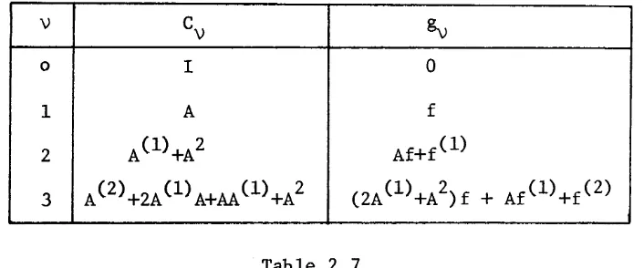
S i n c e t h e f u n c t i o n s C(t) and g ( t ) w i l l c o n t i n u e t o a p p e a r , we need t o d e f i n e t h e s e q u a n t i t i e s i n more g e n e r a l i t y . The u s u a l procedure w i l l b e t o e v a l u a t e y ( p ) ( t ) i n terms of d e r i v a t i v e s and combinations of A ( t ) , f ( t ) and y ( t ) . For s i m p l i c i t y , w e d e f i n e

where C ( t ) i s a n n x n m a t r i x and g ( t ) i s an n-vector.

v

Thus,

Y ( 0 ) ( t ) = y ( t ) => Co = I, go = 0

.

The terms of p a r t i c u l a r i n t e r e s t a r e c o n t a i n e d i n t h e f o l l o w i n g t a b l e .

Table 2.7

I n t h e n e x t s e c t i o n , t h i s method w i l l b e improved upon i n t h e s e n s e t h a t t h e f u n c t i o n s Co, C1, C 2 , and C w i l l b e used t o d e f i n e a s i x t h -

3

order-method.

2. Q u a d r a t u r e Employing (2.1) we g e t

where y ( t ) i s t h e e x a c t s o l u t i o n t o ( l . l a , b ) . I f we a p p l y t h e t r a p e z o i d a l r u l e t o ( 2 . 9 ) , t h e r e s u l t i s

T h i s may b e e q u i v a l e n t l y w r i t t e n a s

u s i n g t h e f u n c t i o n s i n T a b l e 2.7. T h i s one-step method and o t h e r s of a r b i t r a r i l y h i g h o r d e r may b e d e r i v e d i n a more g e n e r a l s e t t i n g by means of (2.9)

.

Lemma 2.11. L e t b ( t ) E cdl[a,b]. Also l e t polynomials p i ( t ) b e

d e f i n e d by

wh.e r e

5,

+

,

(2.12a) and, f o r m a l l y , i s

v-1

5

Thus,

Innumerable schemes p r e s e n t themselves by way of t h i s

Lemma. The Euler-Maclarin sum formula may b e d e r i v e d u s i n g polynomials which l o o k l i k e

of a r b i t r a r i l y high o r d e r . A f i f t h - o r d e r method d e f i n e d i n t h i s manner i s

One u n d e s i r a b l e a s p e c t of (2.13) i s e v a l u a t i n g c 4 ( t ) and g ( t ) . I n 4

o r d e r t o employ (2.13) w e must e v a l u a t e ( t )

,

,

,

,

,

,

,

t h e s e f u n c t i o n s .

3. Gap schemes Thus f a r , w e have c o n s i d e r e d s e v e r a l one-step schemes. The c e n t e r e d - E u l e r scheme w a s g e n e r a l i z e d i n S e c t i o n 1 t o a f o u r t h - o r d e r a c c u r a t e scheme. T h i s i n c r e a s e i n a c c u r a c y i s bought a t t h e p r i c e of e v a l u a t i n g AC2) ( t )

,

,

,

t o A(t) and f ( t )

.

r e q u i r e d e v a l u a t i o n of ( t )

,

complexity and computation time, we want t o examine h i g h - o r d e r , one- s t e p methods w i t h a minimum of d e r i v a t i v e s r e q u i r e d .

The c e n t e r e d - E u l e r scheme and t h e T r a p e z o i d a l Rule (2.10) p o s s e s s a n o t h e r u s e f u l p r o p e r t y . Each of t h e s e d i f f e r e n c e schemes h a s a t r u n c a t i o n e r r o r expansion which c o n t a i n s o n l y even powers of 11

For r e a s o n s t h a t w i l l become c l e a r , s e e S e c t i o n 6 on a s y m p t o t i c e r r o r e x p a n s i o n s , w e want t o p r e s e r v e this p r o p e r t y i n c o n s i d e r i n g high- o r d e r methods.

R e c a l l i n g Lemma 2.11, we have the r e s u l t

b

+

f

V=m

I f t h e sequence of polynomials ( p V ( t )

lvmo

-

13y(a) = pV(b) = 0 v=n+l,. ,

.

t h e n a d i f f e r e n c e method of o r d e r 2n can b e d e f i n e d which r e q u i r e s t h e e v a l u a t i o n of A - )

( 1 ,

,

1 n n

Then

a ) ( p v ( t ) ) s a t i s f y conclusion a ) of Lemma 2.11.

Proof: We can r e p l a c e (.2.15a) w i t h

and t h e sequence s a t i s f i e s c o n c l u s i o n a ) of Lemma 2.11.

b.

5

c. Immediate from (2.15a).

d. To prove t h i s p a r t of t h e Lemma, i t i s s u f f i c i e n t t o show t h a t p 2 r ( t ) , r

2

-

2 - b+a

l o s s of g e n e r a l i t y , we assume t h a t

-

-

2

-

tZr

BY

h y p o t h e s i s ,

p

F,

p

3

n

t-l

I

-

(L)

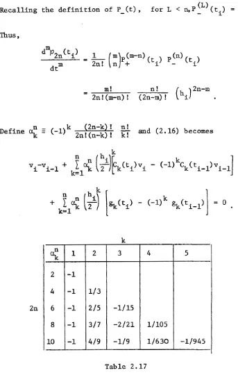
R e c a l l i n g t h e d e f i n i t i o n of P ( t )

,

-

Thus,

-

-

2n! (m-n) ! (2n-m) n! ! ( h i ) 2 n - m *

Define

8

-

(2n-k) !

"I

2n!(n-k)! k!

Table 2.17

Fourth-order scheme:

S i x t h - o r d e r scheme :

The m a t r i c e s C and t h e v e c t o r s gv a r e d e f i n e d i n Table 2.7.

V

D r . K e l l e r n o t e d t h a t t h e s e gap schemes might b e d e r i v e d u s i n g Hermite i n t e r p o l a t i o n t o e s t i m a t e t h e f u n c t i o n

b ( t ) = A ( t ) y ( t )

+

.

For

the

b ( t ) = H(t)

+

-

R e c a l l i n g t h e i n t e g r a l e q u a t i o n (2.1)

,

f f ( t ) may be i n t e g r a t e d e x a c t l y t o g e t

4.

d i f f e r e n c e schemes of t h e form (2.2)

,

,

,

(2.1) s u g g e s t s k - s t e p methods of t h e form

Note t h a t (2.20) r e p r e s e n t s (J-k+l)n e q u a t i o n s i n ( J + l ) n unknowns, and

kn

I1

s t a r t i n g " m-step d i f f e r e n c e schemes, m

<

t h e i n i t i a l - v a l u e matrix,

Ih,

I1

s t a r t i n g " scheme i s of lower o r d e r t h a n t h e k - s t e p method, t h e mesh s i z e , h ( l ) , a s s o c i a t e d w i t h t h e one-step method s h o u l d b e s m a l l e r t h a n t h a t of t h e k-s t e p method, h(k)

.

<

,

5. S t a b i l i t y of T r i a n g u l a r D i f f e r e n c e Schemes A l l of t h e methods mentioned h e r e and most of t h o s e commonly used g i v e r i s e t o b l o c k

i n the form

The f a c t o r of J appearing w i t h a l l M ' s i s a n o r m a l i z a t i o n of t h e

i

i n v e r s e of t h e mesh s i z e . We would l i k e t o examine t h e s t a b i l i t y of f a m i l i e s of m a t r i c e s

1

h

i n i t i a l - v a l u e problems i s well-developed provided t h a t a k-s t e p d i f f e r e n c e scheme i s used and a l l Mij can be w r i t t e n a s

M.

M

1 J i j

s c a l a r . We a r e i n t e r e s t e d i n a r e s u l t which does n o t r e q u i r e t h e s e two r e s t r i c t i o n s on

I

h e

Lemma ( 2 . 2 2 ) . L e t

Ih

.

-1 1

L e t Do b e n o n s i n g u l a r and l e t

I

I I

d ,

I I D ~ I

I=

1 1 ~ ~ 1

I

0

0

and

I

1

-

-

<

0

Proof : T h e matrix

1

-

h

o r , e q u i v a l e n t l y

where

and

-1

By h y p o t h e s i s and the Banach Lemma, D

+

0

I

I

Since (Do

+

+

+

+

Combining C o r o l l a r y 1.27 and Lemma (2.22)

,

Theorem 2.24. L e t t h e l i n e a r boundary-value problem ( l . l a , b ) have a 1

unique s o l u t i o n y ( t ) E C [O,l]. Also, l e t t h e d i f f e r e n c e scheme be pth-order a c c u r a t e . L e t

Bh

-1 1 where M

is

i=O

,

.

.

.

,

I

1

1 1

5

2

,

ii

vv

0

-

I

I M ~ ~ ~

I

5

n

0

and

- 5

1.

<

d 0

-

0

This

a

6. Asymptotic E r r o r Expansions

I n S e c t i o n 3, t h e gap schemes were d e r i v e d s o t h a t t h e t r u n c a t i o n e r r o r expansion would have only even powers of h The

i * advantage of t h i s arrangement w i l l b e e v i d e n t i n t h i s d i s c u s s i o n . The g e n e r a l d i f f e r e n c e scheme i s d e f i n e d a s

The t r u n c a t i o n e r r o r i s h e r e d e f i n e d t o b e

where

z(t)

For example, E u l e r ' s method has t h e t r u n c a t i o n e r r o r , l e t t i n g

-

tR

-

I n g e n e r a l , t h e t r u n c a t i o n e r r o r w i l l be assumed t o b e of t h e form

where e a c h

f

k

k + l which depends, in g e n e r a l n o n l i n e a r l y , upon A ( ~ ) ( t R )

,

Theorem 2.27. Let t h e d i f f e r e n t i a l e q u a t i o n ( l . l a , b ) have a unique s o l u t i o n y ( t ) E

c

Let

b e a s t a b l e , c o n s i s t e n t d i f f e r e n c e approximation t o (1. l a , b )

.

where z ( t ) E C P+l[O,l] and tR = ti

+

.

F k ( ~ ( t )

,

cv

v

midp-k,q-k} .

<

H,

where y o ( t ) = y ( t ) and y k ( t ) , k 1, i s d e f i n e d by

Proof: By i n d u c t i o n and t h e c o n t i n u i t y of

F

,

,

-

i t can b e shown t h a t

Immediately upon s u b s t i t u t i n g

i n t o t h e t r u n c a t i o n e r r o r expansion (2.28b), we g e t

S i n c e yk(t) s a t i s f y (2.30a), we have immediately

and hence

By h y p o t h e s i s , t h e d i f f e r e n c e scheme i s s t a b l e , t h u s

O r e q u i v a l e n t l y ,

The e x p r e s s i o n (2.29) f o r vi

-

1

e r r o r expansion. I n t h e f o l l o w i n g d i s c u s s i o n we assume t h a t

y ( t ) E

cm[O,l],

t r u n c a t i o n e r r o r -ri[z(t)] h a s only even powers of h t h a t i s , i'

F2k+l = 0 , k=O,l,

.

.

.

.

S i n c e t h e d i f f e r e n t i a l e q u a t i o n ( l . l a , b ) h a s a unique s o l u t i o n ,

Assume

,...,

v,

n

B

+

* r-l

b?

"

g

,

" 3 :

a z r t

3

. " ! g

& rl h U 0 k i

k

r l m

+

It

a

$ 8

h *rl 0

U k

a &

8 a a

5

5

"

k 4

- U L )

(I]

*I4

d

3

a (I]

a, * -rl

2 4

because the h. and h

terms

1

i

c l o s e r examination of

F2

F4

d

-

-

[Lz

+

~(A(~)A+A~(~)+~A(~)A(~))

[Lz

1-

Thus,

However, from (2.33) i t can b e s e e n t h a t

Theorem (2.27) and the i d e n t i t i e s ( 2 . 3 3 ) and ( 2 . 3 4 ) show that for t h e Gap6 d i f f e r e n c e scheme

where y 6 ( t ) i s d e f i n e d by

7.

w i l l c o n s i d e r two methods of i n c r e a s i n g

and FOX'S _{method of Deferred C o r r e c t i o n s (Fox} [

2

1,

9

1)

.

Both methods r e l y

on

U

[I]

k rl

'44 Q)

k 3 a Q) 0 0 k a [I] rl

6

5

g

5

3

2

8

5

8

8

3

2

hl \ d I =rl w I n rl I

dfd

?

3 U

disadvantages. At the boundary t=O, the quantity vo must be defined

-1

and thus we have to examine the solution outside the domain of interest.

Also, the solution procedure for

significantly different than

(2.38) where the approximation to the first truncation error term is

included. Evaluation of higher-order derivatives of y(t)

is at best a

delicate procedure and must be done with the utmost care.

Richardson extrapolation avoids these particular problems.

Once two aolutions are calculated, each on a different net, the power

structure of the asymptotic error expansion is used to eliminate the

leading error term at those points common to both nets. For example,

the sixth-order gap scheme has an asymptotic error expansion of the

form

If we solve the discrete problem twice for {vi (1)

3

and {vi(2)

1 ,

then

Let ti(l)

t.

(2), where t

(1)

is the ith point of the first net and

J

i

t

.

(2) is

the

th

point of the second net.

then

This

i s practical, tkat i s , u n t i l the continuity of y ( t ) or round-off

Chapter I11

P a r a l l e l Shooting

T h i s c h a p t e r examines t h e r e l a t i o n s h i p between i m p l i c i t f i n i t e d i f f e r e n c e p r o c e d u r e s and d i s c r e t e i n i t i a l - v a l u e t e c h n i q u e s . The proof of Theorem 1.16 y i e l d s t h e f o l l o w i n g r e s u l t : I f b o t h t h e boundary-value p r o c e d u r e

and t h e i n i t i a l - v a l u e p r o c e d u r e

BV

have un'ique s o l u t i o n s , t h e n

vIV

,

. .

1

p r o c e d u r e ( 3 . 2 a , b , c ) i s a c t u a l l y a method of s o l v i n g t h e e q u a t i o n s ( 3 1 ) The main r e s u l t of t h i s c h a p t e r s t a t e s t h a t any p a r a l l e l s h o o t i n g t e c h n i q u e i s a l s o e q u i v a l e n t t o (3.1) and, t h u s , t o

( 3 . 2 a , b , c ) .

o r t h o g o n a l i z a t i o n p r o c e d u r e ( f o r example, see S e c t i o n 2 on t h e

Method of Complementary F u n c t i o n s ) . W e i n c l u d e a s e p a r a t e t r e a t m e n t of t h e Method of Complementary F u n c t i o n s i n o r d e r t o i l l u s t r a t e

t h e i m p o r t a n t c a s e of s e p a r a t e d boundary c o n d i t i o n s . For completeness t h e Method of A d j o i n t s w i l l b e d i s c u s s e d even though i t h a s no s i m p l e r e l a t i o n s h i p t o (3.1)

.

1. P a r a l l e l Shooting

The boundary-value problem of i n t e r e s t i s

du

- -

d t A ( t ) u

-

(3. 3 )

The s i m p l e s h o o t i n g method (Theorem 1 . 2 ) u s e s t h e s o l u t i o n of (n+l) i n i t i a l - v a l u e problems t o g e n e r a t e t h e s o l u t i o n of ( 3 . 3 a , b ) . I n

p a r a l l e l s h o o t i n g , t h e i n t e r v a l [ o , l ] i s d i v i d e d i n t o K n o n o v e r l a p p i n ~ s u b i n t e r v a l s , [Ty, Tv+l], and s e p a r a t e i n i t i a l - v a l u e problems a r e

s o l v e d on each s u b i n t e r v a l .

he

v

...,

D i s c r e t e p a r a l l e l s h o o t i n g methods mimic t h i s p r o c e d u r e . we p l a c e a n e t ( t y ~ f : ~ on each s u b i n t e r v a l [ T

v-l,

V V

Zo, zo. These n + l i n i t i a l c o n d i t i o n s a r e a r b i t r a r y e x c e p t t h a t

V

we r e q u i r e t h e n x n m a t r i x

Z

0

o r , e q u i v a l e n t l y we w r i t e

V ' V

z

1

z

1

I I

I n p a r a l l e l s h o o t i n g , i t i s sometimes n e c e s s a r y t o s t a t e a n i n i t i a l - v a l u e problem on some i n t e r v a l [T

V '

Tvcl]

f o r m a l l y g i v i n g n + l "boundary" c o n d i t i o n s a t T r a t h e r t h a n v + l

" i n i t i a l " c o n d i t i o n s a t T However, Theoren 1.16 s t a t e s t h a t f o r

v *

a l l n e t s w i t h ho 5 H,

H

zV

0 0

a p p r o p r i a t e l y chosen. Thus, i n o r d e r t o exaniine t h e most g e n e r a l p a r a l l e l s h o o t i n g methods, i t i s s u f f i c i e n t t o c o n s i d e r d i s c r e t e i n i t i a l - v a l u e problems of t h e form (3.4).

V

D e f i n i n g Z

,

v

problem on t h e n e t { t i j i i 0 i s g i v e n by

Thus, t h e c o n t i n u i t y r e q u i r e m e n t s f o r p a r a l l e l s h o o t i n g a r e

Combining ( 3 . 5 ) , ( 3 . 6 ) , (3.,7), and (3.8), t h e p a r a l l e l s h o o t i n g s o l u t i o n ,

vPS,

S t a b i l i t y . For t h e p u r p o s e s of t h i s d i s c u s s i o n , t h e d i s c r e t e p a r a l l e l initial

value

to

I n t h e p r o o f s t o f o l l o w , d e f i n e t h e nJv x n ( J +1) m a t r i x

v

V

The i n i t i a l - v a l u e m a t r i x

I

shoot in^

procedure i s

For convenience, we w i l l w r i t e t h i s m a t r i x a s (K = 3 )

where t h e (1,o) block element of M' i s t h e (SV+2, Sv+l) block element of

1

1

c

Let t h e d i f f e r e n c e scheme be c o n s i s t e n t w i t h (3.3a). Then t h e following a r e e q u i v a l e n t :

a)

v

-

By h y p o t h e s i s

I

I

I

v

1

1

1

1

IK

,

11-

a)

=>

rh,

M

By u s i n g t h e F a c t o r i z a t i o n Lemma (1.12), t h e Reducing Lemma ( 1 . 1 3 ) , and t h e convergence of t h e i n i t i a l - v a l u e problem, i t c a n b e shown t h a t

where K i s independent of ho.

1

1 2 3

L e t V , V , V b e nJ1, n ( J + I ) , n J v e c t o r s r e s p e c t i v e l y .

2 3-

Consider t h e n ( J + l ) e q u a t i o n s

where g2 i s any n ( J 2 + 1 ) - v e c t o r . S i n c e

7

,

2

g2 t h e r e i s a V s u c h t h a t

R e c a l l i n g ( 3 . 1 4 ) , we f i n d t h a t

Thus,

T h i s argument i s v a l i d f o r any

v

...,

v

B e f o r e p r o c e e d i n g w i t h t h e theorem which w i l l t i e a l l t h r e e of t h e s e d i s c r e t e methods t o g e t h e r , i t i s c o n v e n i e n t t o p r e s e n t two lemmas.

Lemma 3.17. L e t C1, C b e n o n s i n g u l a r m x m m a t r i c e s . L e t C1 and

-

C2 b e r e l a t e d by

where L, N a r e m x q , q x m m a t r i c e s r e s p e c t i v e l y . F u r t h e r , l e t L have r a n k q I m. Then t h e q x q m a t r i x [ I

+

P r o o f . By h y p o t h e s i s C1 i s n o n s i n g u l a r , t h e r e f o r e f o r e a c h b E E?,

t h e r e e x i s t s a unique m-vector, x, s u c h t h a t

R e c a l l i n g ( 3 . 1 8 ) , t h i s e q u a t i o n c a n b e r e w r i t t e n a s

o r e q u i v a l e n t l y a s

The Reducing Lemma (1.13) s t a t e s t h a t (3.19) o n l y h a s s o l u t i o n s of t h e form

S i n c e a u n i q u e x, s o l u t i o n of (3.19), e x i s t s f o r e v e r y b , t h e m a t r i x ( I

+

Lemma 3.20. L e t t h e ~ ( J + K ) x ~ ( J + K ) expanded boundary-value m a t r i x

-

8'

L e t t h e boundary-value mat r i x

Bh

.

P r o o f . Suppose t h a t

B~

h

E

V such t h a t

E

However, i f we d e l e t e t h e K-1 e l e m e n t s

v

v

...,

E

By h y p o t h e s i s

Rh

1

[ v [

1

E

each element

vE

and vE a p p e a r s a s a n element of V. Thus, i-1

E

and by c o n t r a d i c t i o n , w e have 8 n o n s i n g u l a r . h

m

Now, w e s t a t e and prove t h e main theorem o f t h i s C h a p t e r , which w i l l i n c l u d e Theorem 1.16.

1

Theorem 3.22. L e t ( 3 . 3 a , b ) have a unique s o l u t i o n y ( t ) E

c

.

L e t t h e d i f f e r e n c e scheme employed b e c o n s i s t e n t w i t h (3.3a). Denote by B V ,

IV,

BV. D i s c r e t e boundary-value p r o c e d u r e , (3.1)

,

Then, f o r a l l n e t s w i t h ho 5 11, H s u f f i c i e n t l y s m a l l ,

i) Each method u n i q u e l y d e f i n e s a n n ( J + l ) v e c t o r as an approximation t o y ( t ) on t h a t n e t , and

Proof: Note that stability

of (3.1) is equivalent to (3.2a)

or (3.9a).

Re

i).

Theorem 1.16 proves that methods

and

IV

uniquely

define approximations to y(t).

To show that method PS uniquely

defines an approximation it is sufficient to show that

nK

nK

matrix in (3.9b) is nonsingular. Without loss of generality, we

consider the case where

3. Thus, we want to show that the

3n

3n matrix

P,

defined by

is nonsingular. From conclusion i),

Bh

is nonsingular, hence by

E

Lemma 3.20,

8

is nonsingular. Recall the n(J+l)-vector

in

E

(3.la), and define the ~(J+K)-vector r by

Consider the matrix equation

R e c a l l i n g t h e p a r a l l e l s h o o t i n 3 method [ 3 , 9 a , b , c ) , eq-uation (3.23) can b e w r i t t e n a s

where

and

-

I n z e n e r a l , L i s a n(J+K)x nK 1 n a t r i x ,

<

+

+

i s n o n s i n g u l a r , where

When t h e p r o p e r s u b s t i t u t i o n s a r e made, i t i s c l e a r t h a t (I

-

NL)

vBV

vIV*

where t h e n-vectors, wi, must s a t i s f y

Now, we have t h e r e l a t i o n s h i p

and thus

is clear that

IV

vps

vBv =

v

Unfortunately, Theorem (3.22) contains no information on

the numerical stability of any parallel shooting technique. To

say that a unique solution to the difference equations (3.9a,b,c)

exists is not to say that it can be accurately approximated

numerically. It is well-known that a simple shooting method may

produce disastrous numerical solutions if the linearly independent

solutions of (3.3a) grow at different rates. For example, consider

the problem

This problem has a unique solution for all f(t)

c[o,l] and

2

f3 E

E

,

because the matrix

1

+

e

1

[Bo

+

BIX(l)

1

1

-..]

l + e

l + e

is nonsingular. However, if we try to invert this matrix numerically,

on a machine with less than 85-bit accuracy, the computer will

be numerically singular due to round-off error. For this reason,

methods which are equivalent

the sense of Theorem 3.22 may yield

greatly different numerical solutions.

2. Method of Complementary Functions

The Method of Complementary Functions (Goodman and Lance

[ 3 ] )

is used to approximate the solution of (3.3a,b) when the boundary

conditions are separated. That is, the boundary conditions (3.3b)

can be written as

where Bo is a

n matrix of rank

is a

n matrix of rank

1

q y p

+

q

n, and Bo,

B1

are a p-vector, q-vector respectively. In

this section, we use the convention that a single matrix in parentheses,

(B,),

has p rows and a single matrix in brackets,

[B

1, has

rows.

The original equations (3.3a9b) can now be rewritten as

In what follows, we assume that the boundary-value problem (3.27ayb)

has a unique solution y(t).

If the boundary-value problem has

a

unique solution, then there exists

vector

such that

0

(Do)qo

(Bo)

where q o

is orthogonal to the null space of

Let the orthonormal

s e t { ~ ~ } z = ~ span t h e n u l l s p a c e of (Bo), t h e n

(qi, ?'lo) = 0 1 s i S q .

With t h e s e n o t i o n s i n hand, t h e s o l u t i o n of (3,27a,b) c a n b e c h a r a c t e r i z e d i n t h e f o l l o w i n g way. S o l v e t h e q homogeneous i n i t i a l - v a l u e problems

and t h e inhomogeneous problem

The unique s o l u t i o n of (3.27a9b) i s g i v e n by

where t h e c o n s t a n t s

cii,

I n t h e i n t r o d u c t i o n t o t h i s c h a p t e r , i t was s t a t e d t h a t t h e Method of Complementary F u n c t i o n s i s a s p e c i a l c a s e of p a r a l l e l s h o o t i n g . T h i s i s t h e b e s t p o i n t a t which t o make t h i s r e l a t i o n s h i p c l e a r . P a r a l l e l s h o o t i n g n a t u r a l l y c o n t a i n s t h e c a s e of s i m p l e

and t h e inhomogeneous problem

--

-

+

where C i s a n o n s i n g u l a r n x n n a t r i x and c i s an n - v e c t o r . Now,

where t h e n - v e c t o r i s d e t e r m i n e d by

The r e s u l t of s p e c i a l i z i n g t h e s i m p l e s h o o t i n g p r o c e d u r e ( 3 , 3 2 a , b ) , ( 3 . 3 3 a , b ) , ( 3 . 3 4 ) , (3.35) by t a k i n g

i s t h e Method of Complementary F u n c t i o n s .

(3.29a,b), (3.30), and (3.31) numerically. Solve the

homogeneous

discrete initial-value problems

and the inhomogeneous discrete initial-value problem

-

-

For convenience, we write (3.32), (3.33) as

c.

-

'li

0

0 L r

i

where Z is

(J+l)n

matrix with its ith column being

.

discrete approximation to

is given

The i n i t i a l - v a l u e e q u a t i o n (3.34) may b e f o r m a l l y w r i t t e n