Adaptive surrogate model based optimization (ASMBO) for unknown groundwater contaminant source characterizations using self-organizing maps

http://www.scirp.org/journal/jwarp ISSN Online: 1945-3108

ISSN Print: 1945-3094

Adaptive Surrogate Model Based Optimization

(ASMBO) for Unknown Groundwater

Contaminant Source Characterizations

Using Self-Organizing Maps

Shahrbanoo Hazrati-Yadkoori

, Bithin Datta

1_{Discipline of Civil Engineering, College of Science and Engineering, James Cook University, Townsville, Australia} 2_{CRC for Contamination Assessment and Remediation of the Environment, CRC CARE, University of Newcastle,}

Callaghan, Australia

Abstract

Characterization of unknown groundwater contaminant sources in terms of location, magnitude and duration of source activity is a complex problem. In this study, to increase the efficiency and accuracy of source characterization an alternative methodology to the methodologies proposed earlier is devel-oped. This methodology, Adaptive Surrogate Modeling Based Optimization (ASMBO) uses the capabilities of Self Organizing Map (SOM) algorithm to design the surrogate models and adaptive surrogate models for source cha-racterization. The most important advantage of this methodology is its direct utilization for groundwater contaminant characterization without the neces-sity of utilizing a linked simulation optimization model. The validation of the SOM based surrogate models and SOM based adaptive surrogate models de-monstrates that the quantity and quality of initial sample sizes have crucial role on the accuracy of solutions as the designed monitoring locations. The performance evaluation results of the proposed methodology are obtained using error free and erroneous concentration measurement data. These results demonstrate that the developed methodology could approximate groundwater flow and transport simulation models, and substitute the optimization model for characterization of unknown groundwater contaminant sources in terms of location, magnitude and duration of source activity.

Keywords

Self-Organizing Map, Surrogate Models, Adaptive Surrogate Models, Groundwater Contamination, Source Identification

How to cite this paper: Hazrati-Yadkoori, S. and Datta, B. (2017) Adaptive Surrogate Mo- del Based Optimization (ASMBO) for Un-known Groundwater Contaminant Source Characterizations Using Self-Organizing Maps. Journal of Water Resource and Protection, 9, 193-214.

https://doi.org/10.4236/jwarp.2017.92014

Received: December 5, 2016 Accepted: February 11, 2017 Published: February 14, 2017

Copyright © 2017 by authors and Scientific Research Publishing Inc. This work is licensed under the Creative Commons Attribution International License (CC BY 4.0).

1. Introduction

Groundwater has a fundamental role in human life as being one of the main re-newable sources of fresh water. Unfortunately, in recent decades, because of in-creasing anthropogenic activities and improper management worldwide, ground- water is subjected to several kinds of pollutants such as seepage from: chemical and petrochemical infrastructure; waste water collection systems; industrial, mining and agriculture fields. However, usually groundwater contamination remains undetected for a long time and is often detected accidently by changing qualities of regional surface water or by chemical analysis of water collected from drinking water wells. Therefore, identifying the unknown characteristics of these contaminant sources and remediation of contaminated groundwater is a necessity. On the other hand, identifying unknown groundwater contaminant source characteristics (contaminant magnitudes, locations and time releases) usually are time consuming and inaccurate because of the uncertainties in the available hydrogeologic information and sparsity of measurement data. Also, the solutions may be non-unique because of high sensitivity to the monitoring data and model parameters. The methodologies proposed earlier to identify unknown groundwater contaminant characteristics can be classified into two major groups: methods based on statistical estimation, and methods based on optimization ap-proaches. An extensive literature review of these methodologies can be found in

[1]-[6]. In the approaches based on optimization, the most effective method to tackle this problem is the linked simulation optimization approach. The linked simulation optimization procedures consist of two main components: 1) models for simulation of groundwater flow and contaminant transport processes, 2) op-timization model with an opop-timization algorithm. Some of the opop-timization

al-gorithms utilized are linear programming and multiple regressions technique [7];

a nonlinear optimization model with embedding technique [8] [9] [10]; Genetic

Algorithm (GA) [11] and [12]; the Artificial Neural Network (ANN) [13] and

[14]; a hybrid methodology based on GA [15] and [16]; the classical nonlinear

optimization algorithm [17]; Simulated Annealing (SA) [18] [19] [20] [21] and

Adaptive Simulated Annealing (ASA) [22], Genetic Programming (GP) [23] and

[24]; ASA in conjunction with uncertainty modeling [25] and [26]. Applica-

tion of these methodologies to real-world cases is generally computationally time intensive, and may need days or weeks of CPU time to obtain an optimal solu-tion.

Therefore, Surrogate Modeling Based Optimization (SMBO) methodologies have been proposed to reduce these enormous computing costs and time asso-ciated with repeated runs of the numerical simulation models within the opti-mization algorithm. Surrogate models based on ANN, GA, Kriging, and regres-sion techniques have been proposed as approximate simulators of the physical

processes [27]. Surrogate models are trained by using numerical simulation

optimi-zation simulation models linked using surrogate models [12]. Using surrogate models can substantially reduce computational time, as the linked simulation optimization models require a repeated solution of the simulation models. Therefore, replacing the numerical simulation models by surrogate models can

result in very substantial computational efficiency and feasibility [28]. In the

present study, an alternative approach to the linked simulation optimization model and SMBO for optimal characterization of unknown groundwater con-taminant sources is proposed and evaluated for potential applicability. In this methodology, the linked simulation optimization model is replaced by a trained Self Organizing Map (SOM) based surrogate model or adaptive surrogate model to characterize unknown groundwater contaminant sources. This methodology: Adaptive Surrogate Modeling Based Optimization (ASMBO) uses the capabili-ties of SOM algorithm to design the surrogate models, and adaptive surrogate models to improve the efficiency of solving the inverse problem of source cha-racterization. The surrogate models approximate the groundwater flow and transport simulation models and the ASMBO eliminates the need for using a formal optimization model for source characterization in terms of location, magnitude and duration of source activity. The specific, main objective of this study is to develop an efficient methodology to characterize unknown ground-water contaminant sources especially where measurement data are sparse and erroneous.

2. Methodology

2.1. Groundwater Flow and Transport Simulation Models

In this study, the numerical simulation model MODFLOW is utilized to simu-late groundwater flow process in a contaminated aquifer. The governing equa-tion in this numerical simulaequa-tion model can be represented by Equaequa-tion (1). This equation describes three-dimensional movement of groundwater in non-

equilibrium, anisotropic and heterogeneous conditions [29]. Analytical solution

of Equation (1), except in a few simple cases, is very difficult. Therefore, to solve Equation (1), different numerical models are applied to reach approximate solu-tions. MODFLOW uses the finite-difference method to solve Equation (1).

xx yy zz s

h h h h

K K K W S

x x y y z z t

 

∂  ∂ ₊ ∂ ∂ ₊ ∂  ∂ _{± =} ∂

 

   

∂  ∂  ∂  ∂  ∂  ∂  ∂ (1)

where:

xx

K , Kyy, and Kzz are the hydraulic conductivity along the x, y, and z

coordinate axes, (L/T);

h is the potentiometric head (L);

W is a volumetric flux per unit volume from aquifer as sources (sinks), the

negative value represents withdrawal of the groundwater system and vice versa (T−1_);

Moreover, for simulating the three dimensional transports of contaminants in groundwater MT3DMS is utilized. The governing equation of MT3DMS can be described by Equation (2), which is a partial differential equation and considers

the fate and transport of contaminants of species k in a 3-D, transient

ground-water flow system [30].

( )

(

)

k k

ij i s s n

j j i

C _C

D v C q C R

t x x x

θ

θ

θ

∂ _∂  _∂  _∂

= _ _− + +

∂ ∂ _ ∂ _ ∂

∑

where

θ

k

C is the concentration of species k which dissolved in groundwater, ML−3;

t is time;

, i j

x x is the distance along the respective Cartesian coordinate axis, L;

ij

D is the hydrodynamic dispersion coefficient tensor, L2T−1;

i

v is the seepage velocity, LT−1;

s

q is volumetric flow rate per unit volume of groundwater system which

represent fluid source (positive) and sinks (negative), T−1_;

k s

C is the concentration of the source or sink flux for species k, ML−3; and

n

R

∑

In this equation, advection, dispersion and chemical reaction of contaminants in groundwater are considered. To solve this equation, the seepage velocity that

is related to the Darcy flux through the relationship i

i

q v

θ

= , should be known.

Therefore, calculating the hydraulic head using MODFLOW is necessary.

2.2. Self-Organizing Map

The Self Organizing Map (SOM) is an algorithm introduced by Kohonen to vi-sualize multidimensional data. This algorithm vivi-sualizes complex non-linear

sta-tistical multidimensional data problems usually into two dimensional display [31]

and [32]. This algorithm transforms the high dimensional data to low

dimen-sional data by preserving the main characteristics and relationships of the input

data [33]. Therefore, the capabilities of SOM algorithm in reducing the

dimen-sions and visualizing of data leads this algorithm to be widely used in various complex fields of sciences such as: statistics, data mining, machine learning

sig-nal processing, financial asig-nalyses, chemistry and social networks [32] and [34].

The SOM algorithm consists of a set of processing units, “neurons”, which are commonly arranged in a 2-dimensional rectangular or hexagonal grid. These neurons are accompanied with a location and a weight vector that connects in-put to outin-put by stating an initial random weight in several iterations to reach a stable map. In other words, this algorithm tries to cluster training data based on

similarity and topology without any external supervision [35]. The main steps of

Kohonen’s SOM algorithm are initialization, competition, cooperation and

adaptation [35] [36] [37] [38], which are described as follows:

units is represented by X:

{

}

as M neurons Y:

{

}

will map to the corresponding units in the input space. The connection weight

vector between input units i and output neurons j can be written as Wj:

}

{

2) Competition: for each input pattern Xi, the output neurons compete to declare the winner neuron. The winner neuron or Best Matching Unit (BMU) is the closest neuron or most similar one to the input vector. The discriminant function used for this step can be defined by Equation (3) which is a squared

Euclidean distance between the input vector X and weight vector Wj.

( )

(

(

)

)

1

min N 1, ,

j i i ji

d x =

∑

3) Cooperation: according to the results of neurobiological studies there is a lateral interaction within a set of excited neuron and the winner neuron. This interaction decays with distance. Therefore, the winning neuron and its topo-logical neighbours update all weights according to Equation (4) and are moved to decrease their distance with the input units.

( )

( ) ( )

( )

ji ji i j i

W =w t +η t K j t _X −W t _ (4)

where

η

( )

( )

neigh-bourhood function.

4) Adaptation: the excited neurons decrease their discriminant function values to reach an appropriate alignment to the input pattern. For this step, the process repeats steps 2 to 4 until the feature map stops changing.

The SOM algorithm visualizes nonlinear relationship of high dimensional da-ta into low dimensional display by preserving the main characteristics of input data. This algorithm is capable of not only clustering and visualizing high di-mensional data but, also is capable of generalization. In other words, SOM can interpolate between the initial data and predict missing values of the system’s

vectors [33]. Figure 1(a) illustrates the process of SOM algorithm in clustering

(a)

(b)

Figure 1. (a) The SOM algorithm for clustering and visualization; (b) The prediction

and visualization. Figure 1(b) shows how this algorithm is utilized for predict-ing the misspredict-ing components of a new vector (Z) of the system based on its known components. In this study, Z represents the vector of measured concen-trations and unknown contaminant sources that need to be estimated. The

soft-ware “SOM Toolbox for Matlab 5” [39] is utilized for constructing the SOM

based surrogate model and the SOM based adaptive surrogate model.

2.3. Application of Adaptive Surrogate Model Based Optimization

for Source Characterization

Surrogate models function essentially by developing a relationship between the inputs and outputs of the system based on training of the model. If this model is constructed accurately, approximates can mimic the behavior of more

sophisti-cated simulation models at substantially reduced computational time [40].

Sev-eral methodologies have been developed to improve the accuracy and efficiency of surrogate modelling such as: Adaptive Surrogate Model Based Optimization (ASMBO). This methodology utilizes adaptive training of the surrogate models

[41] and has been suggested as an efficient methodology to solve time-consum-

ing computer models. The main idea of this procedure is that the direct optimi-zation is substituted by an iterative process comprised of construction,

optimiza-tion and updating of the surrogate model [42]. Moreover, by using adaptive

sampling which is based on the preliminary results of surrogate model, the effi-ciency of the surrogate models is increased. In ASMBO, after sampling a certain number of selected parameters sets in initial stage, additional sampling which can effectively increase the accuracy of the surrogate model results are added. An adaptive sampling methodology improves the speed of obtaining the accurate

variable values [43]. In this study, a new type of ASMBO is developed to

charac-terize unknown groundwater contaminant sources. This developed methodology is SOM based surrogate model or SOM based adaptive surrogate model which is utilized to characterize unknown groundwater contaminant sources in terms of

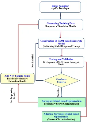
location, magnitude and activity time. Figure 2 illustrates the main stages of

constructing a SOM based surrogate model and SOM based adaptive surrogate model for source identification. These stages are briefly discussed in the follow-ing paragraphs.

1) Initial sampling: first, the main variables of the defined system as per their

degree of importance, according to the preliminary experiments are chosen [44].

The main question in this stage is how we could design our surrogate models to accurately mimic the behavior of the defined system with limited numbers of inputs. Furthermore, Latin Hypercube Sampling (LHS) is appropriate and

suita-ble for this stage [45]. In this stage, it is crucial to ensure sampling is selected

through all domains of input values and due to this characteristic LHS is utilized in this study. Also, the upper and lower bounds of these variables are assumed to be known.

Figure 2. Key elements of the Adaptive Surrogate Model based Optimization (ASMBO) procedure for source identification as an inverse method.

stage. In this study, the groundwater flow and transport simulation models MODFLOW and MT3DMS (within GMS 7) are solved for randomly generated source fluxes.

3) Construction of surrogate model: in this stage, Self-Organizing Map (SOM) is utilized as the surrogate model type to represent the response surface of the simulation model inputs-outputs values. The other main issue in this stage is how the selected variables are used to design the SOM based surrogate model.

4) Testing and validation: this stage evaluates the potential applicability of the surrogate models. The new randomly generated sample sets that were not used in the training process are utilized in this stage. The results are applicable for modification of the surrogate model type and its design. The performance of the SOM based surrogate model is evaluated for two conditions: first, it is assumed that the contaminant concentration values at specific time and locations are known and the corresponding contaminant source fluxes at specified potential locations at specific time are considered as unknown variables to be estimated.

Generating Training Data

Responses of Simulation Models

Construction of SOM based Surrogate Model

(Initializing Model Design and Traing)

Testing and Validation

Development of SOM based Surrogate Model

Goodness Criteria

N

o

t S

a

ti

sfi

ed

S

a

ti

sfi

ed

Surrogate Model based Optimization

Preliminary Source Characterization

F

or

I

m

p

rovi

n

g

Re

su

lt

s

Add New Sample Points

Based on Preliminary Estimation Results

Adaptive Surrogate Model based Optimization

(Source Characterization)

Initial Sampling

Second, the constructed SOM based surrogate model performance is also tested by estimating spatial and temporal concentration values at specified time and locations, assuming contaminant sources are known.

In this stage, the BMU which has similar definition (Equation (3)) as the im-plicit objective function of source identification problem is utilized to character-ize unknown contaminant sources of testing sample sets as an inverse problem. The implicit objective function of source identification problem is defined to minimize the difference between estimated contaminant concentration values and observed contaminant concentration values at specific monitoring locations at specific time. The main constraints of optimization model are groundwater flow and transport simulation models. In this proposed methodology, the SOM based surrogate models represent approximate simulation of the physical processes. In other words, the obtained BMU of the SOM based surrogate model is utilized to find the unknown characteristics (magnitude, location and duration) of potential contaminant sources, hence eliminating the necessity of using any complex and explicit optimization model.

5) SOM based surrogate model/stage 3: If the solution results are acceptable SOM based surrogate model is selected and it is ready for characterizing un-known contaminant sources as an inverse problem by utilizing BMU; otherwise, go to stage 3 and change the design of surrogate model.

6) Adaptive surrogate model: in this stage, to improve the SOM based surro-gate model results, the adaptive sampling strategy is applied. There are several adaptive sampling methods such as: Maximizing Expected Improvement (MEI), Maximizing the Probability of Improvement (MPI) and Minimizing a Statistical Lower Bound (MSL).

All of these three strategies lead the algorithm to go back and find the areas where the samples point are located. However, in this study instead of the men-tioned strategies new samples based on obtained results of SOM based surrogate model are added to the initial sample sets. This essentially means that additional training patterns are generated utilizing the latest source characterization esti-mates. Then the model is re-trained to effectively increase the accuracy of source identification results.

2.4. Performance Evaluation

In this study, performance of the developed methodology is evaluated utilizing synthetic hydrogeologic and geochemical data for an illustrative contaminated aquifer. The advantage in using synthetic data is that the unknown data errors in the measurement data can be quantified and need not be treated as unknown quantities for evaluation purpose. Normalized Absolute Error of Estimation (NAEE) is also utilized as a measure to calculate a normalized error of

estima-tion. Equation (5) represents NAEE [22]:

( )

( ) ( )

( )

1 1 est act

1 1 _act

NAEE % 100

S N j j

i i

i j

S N j

i

i j

q q

q

= =

= =

−

=

∑ ∑

where:

S is the number of pollution source (s);

N is the number of transport stress periods;

( )

q is actual source flux at source number i in stress period j;

( )

j i

q is estimated source flux at source number i in stress period j.

3. Performance Evaluation of the Developed Methodology

3.1. Study Area

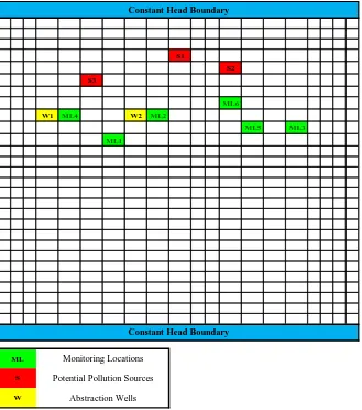
The illustrative study area utilized for the performance evaluation of the pro-posed methodology is a homogeneous aquifer which consists of one confined

layer (Figure 3). Table 1 shows the aquifer characteristic values and dimensions

of this study area. In this study area, the north and south boundaries are consi-dered as specified head boundaries with 35 m and 25 m as specified head for north and south boundaries, respectively. Whereas, the east and west boundaries are variable heads. In this case, only a conservative contaminant is considered and three potential contaminant source locations are considered (S1, S2, and S3). The locations and actual contaminant fluxes of these three potential

conta-minant sources are presented in Table 2. There are six monitoring locations

(ML1 to ML6) and two abstraction wells (W1 and W2); these important features

are shown in Figure 3. The total time of simulation is divided into 5 different

stress periods (SP1 to SP5). The first four stress periods are each of 183 days du-ration, and the last stress period is of 2200 days duration. Potential contaminant sources are assumed to be active only in the first four stress periods. The

ab-straction rates for each stress period at the abab-straction wells are presented in

Ta-ble 3.

Table 1. Hydrogeologic characteristics of the study area.

Parameter Unit Value

Maximum length of study area m 1000 Maximum width of study area m 1500 Saturated thickness, b m 7.6 Grid spacing in x-direction m 50 Grid spacing in y-direction m 50 Horizontal hydraulic conductivity m/d 18 Porosity Dimensionless 0.25 Longitudinal dispersivity m 35

Figure 3. Illustrative study area represents potential contaminant source locations, ab- straction wells and monitoring locations.

Table 2. The locations and actual contaminant fluxes of three potential contaminant

sources.

Potential contaminant source location (row, column)

Contaminant fluxes (Kg/day)

SP1 SP2 SP3 SP4 SP5

S1 (5, 10) 0 0 0 0 0

S2 (6, 13) 60 20 45 50 0

S3 (7, 6) 80 58 22 30 0

Table 3. Abstraction well locations and abstraction rates in different stress periods.

ID Row Column Abstraction rate for each stress period (m 3_/day)

1 2 3 4 5

Abstraction well 1 10 4 −100.25 −100.25 −68 −16 −49

Abstraction well 2 10 8 −100.25 −80.2 −96 −100.25 −88

S1

S2

S3

ML6

W1 ML4 W2 ML2

ML5 ML3

ML1

ML

S

W

Monitoring Locations Potential Pollution Sources

Abstraction Wells

3.2. Application of the SOM Based Surrogate Model for

Source Identification

In this study, SOM based surrogate models and SOM based adaptive surrogate models are utilized to characterize unknown groundwater contaminant sources as an inverse problem. The following steps are followed to select the best SOM based surrogate model among constructed models for illustrative study area; then, the SOM based adaptive surrogate model is developed.

1) Scenarios for initial sampling: LHS is used to randomly generate two groups of 1000 initial sample sets. These sample sets are generated by assuming that all of these three potential sources are active through first four stress periods, SP1 to SP4. Also, three groups of 100 sample sets are generated by assuming that in each group at least one of the sources is inactive. The contaminant source fluxes are assumed to be in the range of 0 - 100 kg/day for all potential sources. For all of the generated sample sets, the three potential contaminant source fluxes at five different stress periods and their corresponding contaminant con-centration magnitudes at specified monitoring locations and specific stress pe-riods are selected as the variables of the surrogate models for this study area.

2) Generating training data: the solution results of the numerical simulation models for generated initial sample sets are obtained in this step. The numerical flow and transport simulation models MODFLOW and MT3DMS (within GMS 7) are solved to obtain adequate sample data for training and testing of the

sur-rogate models. Figure 4 shows a typical contaminant plume 732 days after start

of the first source activity. The training data consist of randomly generated con-taminant source fluxes and their corresponding concon-taminant concentration

val-ues at the specified monitoring locations at specified times. Table 4 represents a

typical input for training of a SOM based surrogate model. This input consists of five sample sets. Each set consists of randomly generated contaminant source fluxes for three potential contaminant sources at four stress periods (SP1 to SP4). Also, it consists of corresponding contaminant concentration magnitudes at six monitoring locations (M1 to M6) at five stress periods (SP1 to SP5).

3) Construction of the SOM based surrogate model: in this step, SOM algo-rithm is utilized to create SOM based surrogate models. It is supposed that if SOM based surrogate models are constructed accurately, these models could properly approximate the groundwater flow and transport simulation models.

Table 4. Typical input vectors for training a SOM based surrogate model.

Source fluxes (Kg/day) Contaminant concentration (g/l)

S1-SP … M1-SP …

1 2 3 4 … 1 2 3 4 5 …

Figure 4. A typical concentration plume 732 days after start of first source activity.

4) Testing and validation of the SOM based surrogate model: the constructed SOM based surrogate models are tested by 100 new random sample sets. The contaminant source fluxes of these sample sets are generated randomly by using LHS method in the range of 0 - 100 kg/day. Then, the corresponding contami-nant concentration values at monitoring locations are obtained by utilizing the simulation models. In this stage, different surrogate models representing differ-ent numbers of initial sample sizes, and SOM map units are constructed and evaluated. The evaluation results lead to selection of the best candidate SOM based surrogate model among the constructed surrogate models for the illustra-tive study area.

As mentioned in the methodology section, because the definition of BMU of the SOM algorithm (Equation (3)) is similar to the definition of the implicit ob-jective function of source identification problem. Therefore, the BMU of SOM algorithm is utilized for estimating unknown characteristics (magnitude, loca-tion and duraloca-tion) of potential contaminant sources. This algorithm by using the information of known components of the input vector estimated the unknown components of the input vector. In this study, this capability of the SOM algo-rithm is utilized to characterize unknown groundwater contaminant sources as an inverse problem. It also utilized to estimate contaminant concentration values at specified location and time when the contaminant sources and their characte-ristics are known.

For performance evaluation of source characterization capabilities utilizing the trained SOM surrogate models, the contaminant concentration values at monitoring locations at specific times are considered as known variables of an input vector. This vector needs to have the same number of variables as the

in-put vectors of training phase. Table 5 represents a typical input for testing data

Table 5. A typical input vector with missing data for testing a SOM based surrogate model.

Source fluxes (Kg/day) Contaminant concentration (g/l)

S1-SP S2-SP S3-SP M1-SP …

1 2 3 4 1 2 3 4 1 2 3 4 1 2 3 4 5 0.00 0.04 0.10 0.14 0.00 … 0.00 0.03 0.08 0.16 0.00 … 0.00 0.05 0.13 0.16 0.00 … 0.00 0.02 0.09 0.22 0.00 … 0.01 0.06 0.15 0.24 0.00 …

models. The contaminant source fluxes for three potential contaminant sources at four stress periods (SP1 to SP4) are assumed as unknown variables. The BMU is utilized to estimate these unknown variables. By searching for the BMU and using the information of known components of the input vector, the most simi-lar vector is recognized. Therefore, missing values of the input vector are esti-mated.

5) The selected SOM based surrogate model: the selected SOM based surro-gate model is used to characterize the unknown groundwater contaminated sources as an inverse problem and for further performance evaluation.

6) SOM based adaptive surrogate model: It is supposed that SOM based adap-tive surrogate models could improve the source characterization results. There-fore, based on the preliminary results of the selected SOM based surrogate

mod-el (i.e., emphasizing the preliminary or latest source estimation results new

sam-ple patterns are randomly generated) the SOM based adaptive surrogate model is constructed for contaminated aquifer by adding new sample sets. 500 new sam-ple sets are generated by utilizing LHS and considering the results obtained by utilizing SOM based surrogate model for source identification.

3.3. Results

model for estimating contaminant concentrations at selected monitoring

loca-tions is shown in Figure 5. This figure compares the estimated concentration

values against actual concentration values.

Different SOM based surrogate models representing different numbers of SOM map units are also constructed. In these scenarios, the number of moni-toring locations and the number of initial sample sets are maintained constant at 6 and 2300, respectively. The solution results for source identification and

esti-mating contaminant concentration at monitoring locations are presented in

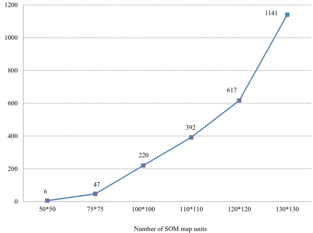
Ta-ble 6. The solution results except for SOM based surrogate model which is con-structed by utilizing 50 × 50 map units demonstrate a consistency in the solution result, and the best results are reached by utilizing 130 × 130 map units. An im-portant constraint in these evaluations of different scenarios is the CPU capacity, which is exceeded by increasing the number of SOM map units beyond 120 ×

120 (Figure 6). Therefore, the SOM based surrogate model which consisted of

Figure 5. The results obtained from SOM based surrogate model for estimating the

contaminant concentration values at selected monitoring locations (NAEE is equal to 15 percent).

Table 6. The performance evaluation of different scenarios representing different

numbers of SOM map units.

ID Number of _{map units}

SOM map characteristics NAEE (%)

Map shape Neighborhood _function (Substituting groundwater flow and SOM based Surrogate Model transport simulation models) 1 50 × 50

Rectangular Gaussian

43.8

2 75 × 75 31.3

3 100 × 100 30.4

4 110 × 110 30.9

5 120 × 120 30.4

6 130 × 130 29.8

0 0.05 0.1 0.15 0.2 0.25 0.3 0.35 0.4 0.45 0.5

M1 (12,7) M2 (10,9) M3 (11,16) M4 (10,5) M5 (11,14) M6 (9,13)

Co

n

ta

m

in

an

t

Co

n

ce

n

tr

at

io

n

(

g

/l

)

Monitoring locations (Row, Column)

Estimated and actual contaminant concentration values at monitoring locations

Figure 6. Required times for developing different SOM based surrogate models repre- senting different numbers of SOM map units.

2300 initial sample sets and 100*100 map units is selected as the best SOM based surrogate model among constructed SOM based surrogate models.

The developed SOM based surrogate models could approximate the ground-water flow and transport simulation models. These outcomes are achieved ac-cording to the solution results obtained at model evaluation and model testing stages. The solution results presented earlier lead to the selection of the most suitable surrogate model among the constructed surrogate models for the illu-strative study area. This model is constituted of 100 × 100 SOM map units that utilized the 2300 initial sample sets. These 2300 random initial sample sets used the information from three potential contaminant sources and the correspond-ing contaminant concentration at 6 existcorrespond-ing monitorcorrespond-ing locations. The obtained solution results for contaminated study area by utilizing the measured contami-nant concentration values at 6 existing monitoring locations are illustrated in

Figure 7. This figure compares the estimated contaminant source fluxes against actual contaminant source fluxes at three potential sources (S1 to S3) at 5 speci-fied stress periods (SP1 to SP5).

The obtained results are not entirely satisfactory and the NAEE is equal to 31 percent. However, the obtained results in this stage demonstrate that the S1 is an inactive source. This result also achieved by other constructed SOM based sur-rogate. Therefore, in order to improve the accuracy of results, it may be neces-sary to incorporate new samples, and possibly construct a SOM based adaptive surrogate model for unknown groundwater contaminant source identification. 500 new sample sets are generated by utilizing LHS and considering that S1 is an inactive source. The solution results for SOM based adaptive surrogate models

are illustrated in Figure 8. The illustrated solution results demonstrate

signifi-cant improvement by generating new samples. For example, the accuracy of

6

47

220

392

617

1141

0 200 400 600 800 1000 1200

50*50 75*75 100*100 110*110 120*120 130*130

R

equie

re

d

ti

m

e f

or

c

onstr

uc

ti

ng

S

O

M

m

aps

(se

c)

Figure 7. The results obtained from the selected SOM based surrogate models for source identification of actual contaminant source fluxes (NAEE is equal to 31 percent).

Figure 8. The performance evaluation of the SOM based adaptive surrogate models and

the selected SOM based surrogate model in terms of NAEE for characterizing unknown contaminant sources, the NAEE are equal to 20 and 31 percent, respectively.

solution results of SOM based adaptive surrogate models increases by 11 percent when compared to the results obtained using the previously selected SOM based surrogate model.

Moreover, for continuing the evaluation of the performance of the developed SOM based adaptive surrogate model and the previously selected SOM based surrogate model, synthetic erroneous concentration measurements data are uti-lized for evaluation purpose. For this purpose, simulated contaminant

concen-trations are perturbed with varied amounts of random errors, i.e., 5, 10, 15, 20,

0 10 20 30 40 50 60 70 80 90 S 1 -S P 1 S 1 -S P 2 S 1 -S P 3 S 1 -S P 4 S 1 -S P 5 S 2 -S P 1 S 2 -S P 2 S 2 -S P 3 S 2 -S P 4 S 2 -S P 5 S 3 -S P 1 S 3 -S P 2 S 3 -S P 3 S 3 -S P 4 S 3 -S P 5 So u rce flu x es ( k g /d ay ) Sources-Stress periods

Actual values Estimated values

0 10 20 30 40 50 60 70 80 90 100 S1 -SP 1 S1 -SP 2 S1 -SP 3 S1 -SP 4 S1 -SP 5 S2 -SP 1 S2 -SP 2 S2 -SP 3 S2 -SP 4 S2 -SP 5 S3 -SP 1 S3 -SP 2 S3 -SP 3 S3 -SP 4 S3 -SP 5 So u rce flu x es ( k g /d ay ) Sources-Stress periods

25 and 30 percent of simulated values. The simulated contaminant concentra-tions measurements at monitoring locaconcentra-tions are assumed to incorporate 5, 10, 15, 20, 25 and 30 percent random errors. The following equation is utilized for syn-thetically generating the perturbed concentration measurement values with

random errors [22].

per S S

C =C + × ×a b C (6)

where

per

C is perturbed concentration measurement values;

S

C is simulated concentration values;

a is maximum deviation expressed as a percentage; and

b is a random fraction between +1 and −1 obtained by utilizing the LHS.

The source characterization results obtained with these erroneous

concentra-tion measurements are shown in Figure 9.

These solution results shown in Figure 9 demonstrate that the source

charac-terization performances do not substantially change for scenarios with error free, 5 percent, 10 percent, 15 and 20 percent concentration measurement errors.

Figure 9 also indicates that the accuracy of estimated source fluxes significantly decreased when the incorporated errors are 25 percent or larger.

3.4. Discussion

The performance evaluation results of the SOM based surrogate model are not entirely satisfactory. These very limited results show that it could approximate groundwater flow and transport simulation models properly. However, for creasing the efficiency of developed methodology additional training with in-corporation of different actual source location scenarios were developed. The evaluation results also indicated that the quantity and quality of initial sample sets and the number of SOM map units have a crucial rule in the efficiency of the

Figure 9. The performance evaluation results of the SOM based surrogate models and

SOM based adaptive surrogate models in terms of NAEE. 0

10 20 30 40 50 60

Selected SOM based surrogate model SOM based adaptive surrogate model

N

A

EE (%

)

Error free data 5% uncontrolled errors 10% uncontrolled errors 15% uncontrolled errors

model (Table 6 and Figure 6). In order to improve the accuracy of the solution results, the following strategies are suggested:

1) Using the concentration data at designed monitoring locations, designed

for improving source characterization [24] [46] [47]. For example, for this study

area if the contaminant concentration values of 20 monitoring locations which recorded larger concentrations are utilized; the results for SOM based surrogate model improved by 12 percent. Selections of adequate and relevant monitoring locations are necessary, especially if the contaminant plumes from some of the potential sources overlap.

2) Exploring other methods to generate initial random sample sets;

3) Utilizing optimal number of variables in the designing of surrogate models by selecting only those available monitoring locations which affect the accuracy of identifying pollution sources; and

4) Applying sequential sampling method as in SOM based adaptive surrogate models by considering the previous stage results.

It can be concluded that, SOM based surrogate model and SOM based adap-tive surrogate model could be utilized to identify unknown characteristics of po-tential contaminant source in contaminated aquifers. Also, these could be ap-plied to estimate the contaminant concentration values at specified monitoring location if the contaminant sources are known. Especially, additional informa-tion based on earlier estimates of the contaminant source characteristics scena-rios if incorporated in the training stage; it can increase the efficiency in terms of more accurate estimation when new samples are added. This is essentially the adaptive surrogate model based optimization approach. One of the advantages of this methodology is the consistency of solution results for ideal (error free concentration measurements) and real (when contaminant concentration in-corporate up to 20 percent erroneous data) scenarios. This observation may be relevant only when limited numbers of initial samples are utilized. Therefore, the selected method to generate relevant initial sample sets has important role on the solution results. Also, utilizing sufficient size of sample sets is necessary.

4. Conclusions

Different scenarios correspond to different surrogate models with various num-bers of initial sample sizes and Self-Organizing Map (SOM) map units are con-sidered. Also, the performance of the developed methodology is evaluated by utilizing the SOM based surrogate model, to identify potential contaminant sources, for an ideal scenario of error free concentration data, as well as scena-rios with different degrees of erroneous concentration measurements data. In

addition, an improved version of SOM based surrogate model, i.e. SOM based

adaptive surrogate model (ASMBO) is constructed to characterize potential contaminant sources. Main conclusions that can be drawn from these limited performance evaluation results are:

me-thodology can be used as an alternative meme-thodology for unknown groundwater contaminant sources characterization, which can potentially eliminate the

ne-cessity of using other widely used methodologies, i.e., the linked simulation

op-timization methodology.

2) The quality of initial sample size is important. This size should be adequate and cover the whole plausible range of contaminant source fluxes for all the po-tential contaminant sources.

3) The size of SOM map units is important. The best size should be selected due to the memory of PC used, number of variables, and initial sample sizes.

4) The performance evaluation results do show comparatively large errors in terms of the specific error criteria utilized. However, a comparison of the source estimates and the actual source characteristics shows a good match.

5) Most important conclusion is that the SOM based surrogate models may provide a feasible methodology for characterization/identification of unknown groundwater contaminant sources in terms of location, magnitude and duration of source activity, without the necessity of using a linked simulation optimiza-tion model, when the ASMBO methodology is adopted. However, it appears likely that the accuracy of characterization may not be adequate in real life sce-narios with multiple sources, complex hydrogeology of the aquifer, and parame-ter estimation uncertainties.

6) The SOM based models seem to perform satisfactorily when concentration measurement data are erroneous.

7) The performance evaluation results presented in this study are very limited in scope and more rigorous evaluations are necessary to establish its applicability for source identification without using any optimal decision model. These per-formance evaluation results are based on very limited scenarios. More rigorous performance evaluations incorporating: random heterogeneity of hydrogeologic parameters and considering more complex geochemical processes are necessary to establish the applicability of the proposed methodology.

Acknowledgements

The second author thanks CRC-CARE, Australia for providing financial support for this research through Project No. 5.6.0.3.09/10(2.6.03), CRC-CARE-Bithin Datta which partially funded the Ph.D. scholarship of the first author.

References

[1] Atmadja, J. and Bagtzoglou, A. (2001) State of the Art Report on Mathematical Me-thods for Groundwater Pollution Source Identification. Environmental Forensics, 2, 205-214. https://doi.org/10.1006/enfo.2001.0055

https://doi.org/10.1016/j.jconhyd.2006.06.006

[4] Sun, A.Y., Painter, S.L. and Wittmeyer, G.W. (2006) A Constrained Robust Least Squares Approach for Contaminant Release History Identification. Water Resources

Research, 42, W04414. https://doi.org/10.1029/2005WR004312

[5] Chadalavada, S., Datta, B. and Naidus, R. (2011) Optimisation Approach for Pollu-tion Source IdentificaPollu-tion in Groundwater: An Overview. International Journal of

Environment and Waste Management, 8, 40-61.

https://doi.org/10.1504/ijewm.2011.040964

[6] Amirabdollahian, M. and Datta, B. (2013) Identification of Contaminant Source Characteristics and Monitoring Network Design in Groundwater Aquifers: An Overview. Journal of Environmental Protection, 4, 26-41.

https://doi.org/10.4236/jep.2013.45A004

[7] Gorelick, S.M., Evans, B. and Remson, I. (1983) Identifying Sources of Groundwater Pollution—An Optimization Approach. Water Resources Research, 19, 779-790. https://doi.org/10.1029/WR019i003p00779

[8] Mahar, P.S. and Datta, B. (1997) Optimal Monitoring Network and Ground-Water- Pollution Sources Identification. Journal of Water Resource Planning and Manage-ment, 123, 199-207. https://doi.org/10.1061/(ASCE)0733-9496(1997)123:4(199) [9] Mahar, P.S. and Datta, B. (2000) Identification of Pollution Sources in Transient

Groundwater Systems. Water Resources Management, 14, 209-227. https://doi.org/10.1023/A:1026527901213

[10] Mahar, P.S. and Datta B. (2001) Optimal Identification of Ground-Water Pollution Sources and Parameter Estimation. Journal of Water Resources Planning and Man-agement-Asce, 127, 20-29.

https://doi.org/10.1061/(ASCE)0733-9496(2001)127:1(20)

[11] Aral, M.M., Guan, J.B. and Maslia, M.L. (2001) Identification of Contaminant Source Location and Release History in Aquifers. Journal of Hydrologic Engineer-ing, 6, 225-234. https://doi.org/10.1061/(ASCE)1084-0699(2001)6:3(225)

[12] Singh, R.M. and Datta, B. (2006) Identification of Groundwater Pollution Sources Using GA-Based Linked Simulation Optimization Model. Journal of Hydrologic

Engineering, 11, 101-109. https://doi.org/10.1061/(ASCE)1084-0699(2006)11:2(101)

[13] Singh, R.M., Datta, B. and Jain, A. (2004) Identification of Unknown Groundwater Pollution Sources Using Artificial Neural Networks. Journal of Water Resources Planning and Management-Asce, 130, 506-514.

https://doi.org/10.1061/(ASCE)0733-9496(2004)130:6(506)

[14] Singh, R.M. and Datta, B. (2007) Artificial Neural Network Modeling for Identifica-tion of Unknown PolluIdentifica-tion Sources in Groundwater with Partially Missing Con-centration Observation Data. Water Resources Management, 21, 557-572. https://doi.org/10.1007/s11269-006-9029-z

[15] Mahinthakumar, G.K. and Sayeed, M. (2005) Hybrid Genetic Algorithm—Local Search Methods for Solving Groundwater Source Identification Inverse Problems.

Journal of Water Resources Planning and Management, 131, 45-57.

https://doi.org/10.1061/(ASCE)0733-9496(2005)131:1(45)

[16] Mahinthakumar, G.K. and Sayeed, M. (2006) Reconstructing Groundwater Source Release Histories Using Hybrid Optimization Approaches. Environmental Foren-sics, 7, 45-54. https://doi.org/10.1080/15275920500506774

[17] Datta, B., Chakrabarty, D. and Dhar, A. (2011) Identification of Unknown Ground- water Pollution Sources Using Classical Optimization with Linked Simulation. Jour- nal of Hydro-Environment Research, 5, 25-36.

[18] Jha, M. and Datta, B. (2012) Simulated Annealing Based Simulation-Optimization Approach for Identification of Unknown Contaminant Sources in Groundwater Aquifers. Desalination and Water Treatment, 32, 79-85.

[19] Prakash, O. and Datta, B. (2014) Characterization of Groundwater Pollution Sources with Unknown Release Time History. Journal of Water Resource and Pro-tection, 6, 337-350. https://doi.org/10.4236/jwarp.2014.64036

[20] Prakash, O. and Datta, B. (2014) Optimal Monitoring Network Design For Efficient Identification of Unknown Groundwater Pollution Sources. International Journal of

GEOMATE, 6, 785-790.

[21] Prakash, O. and Datta, B. (2015) Optimal Characterization of Pollutant Sources in Contaminated Aquifers by Integrating Sequential-Monitoring-Network Design and Source Identification: Methodology and an Application in Australia. Hydrogeology Journal, 23, 1089-1107. https://doi.org/10.1007/s10040-015-1292-8

[22] Jha, M. and Datta, B. (2013) Three-Dimensional Groundwater Contamination Source Identification Using Adaptive Simulated Annealing. Journal of Hydrologic

Engineering, 18, 307-317. https://doi.org/10.1061/(ASCE)HE.1943-5584.0000624

[23] Datta, B., Prakash, O., Campbell, S. and Escalada, G. (2013) Efficient Identification of Unknown Groundwater Pollution Sources Using Linked Simulation-Optimiza- tion Incorporating Monitoring Location Impact Factor and Frequency Factor. Wa-ter Resources Management, 27, 4959-4976.

https://doi.org/10.1007/s11269-013-0451-8

[24] Prakash, O. and Datta, B. (2013) Multiobjective Monitoring Network Design for Ef-ficient Identification of Unknown Groundwater Pollution Sources Incorporating Genetic Programming–Based Monitoring. Journal of Hydrologic Engineering, 19. https://doi.org/10.1061/(ASCE)HE.1943-5584.0000952

[25] Amirabdollahian, M. and Datta, B. (2014) Identification of Pollutant Source Charac- teristics Under Uncertainty in Contaminated Water Resources Systems Using Adap- tive Simulated Anealing and Fuzzy Logic. International Journal of GEOMATE, 6, 757-762.

[26] Amirabdollahian, M. and Datta, B. (2015) Reliability Evaluation of Groundwater Contamination Source Characterization under Uncertain Flow Field. International Journal of Environmental Science and Development, 6, 512-518.

https://doi.org/10.7763/IJESD.2015.V6.647

[27] Razavi, S., Tolson, B.A. and Burn, D.H. (2012) Review of Surrogate Modeling in Water Resources. Water Resources Research, 48, W07401.

https://doi.org/10.1029/2011WR011527

[28] Datta, B. and Kourakos, G. (2015) Preface: Optimization for Groundwater Charac-terization and Management. Hydrogeology Journal, 23, 1043-1049.

https://doi.org/10.1007/s10040-015-1297-3

[29] Harbaugh, A.W. (2005) MODFLOW-2005, the U.S. Geological Survey Modular Ground-Water Model—The Ground-Water Flow Process. U.S. Geological Survey Techniques and Methods 6-A16.

[30] Zheng, C. and Wang, P.P. (1999) MT3DMS: A Modular Three-Dimensional Mul-tispecies Transport Model for Simulation of Advection, Dispersion and Chemical Reactions of Contaminants in Groundwater Systems; Documentation and User’s Guide. Contract Report SERDP-99-1, US Army Corps of Engineers-Engineer Re-search and Development Center, 220.

[31] Kohenon, T., et al. (1996) Engineering Applications of the Self-Organizing Map.

[32] Kohonen, T. (2001) Self-Organizing Maps. Springer-Verlag, Berlin Heidelberg. [33] Simula, O., Alhoniemi, E. and Vesanto, J. (1999) Analysis and Modeling of

Com-plex Systems Using the Self-Organizing Map. 1-16.

[34] Thi, H.A.L. and Nguyen, M.C. (2014) Self-Organizing Maps by Difference of Con-vex Functions Optimization. Data Mining and Knowledge Discovery, 28, 1336- 1365. https://doi.org/10.1007/s10618-014-0369-7

[35] Dragomir, O.E., Dragomir, F. and Radulescu, M. (2014) Matlab Application of Ko-honen Self-Organizing Map to Classify Consumers’ Load Profiles. Procedia Com-puter Science, 31, 474-479. https://doi.org/10.1016/j.procs.2014.05.292

[36] Bullinaria, J.A. (2004) Self Organizing Maps: Fundamentals (Introduction to Neural Networks: Lecture 16).

[37] Bullinaria, J.A. (2004) Self Organizing Maps: Algorithms and Applications (Intro-duction to Neural Networks: Lecture 17).

[38] Bullinaria, J.A. (2014) Self Organizing Maps: Properties and Applications (Neural Computation: Lecture 17).

[39] Vesanto, J., Himberg, J., Alhoniemi, E. and Parhankangas, J. (2000) SOM Toolbox for Matlab 5, in Report A57. SOM Toolbox Team, Helsinki University of Technol-ogy, Finland, 1-60. http://www.cis.hut.fi/projects/somtoolbox

[40] Gorissen, D., et al. (2010) A Surrogate Modeling and Adaptive Sampling Toolbox for Computer Based Design. Journal of Machine Learning Research, 11, 2051-2055. [41] Sreekanth, J. and Datta, B. (2010) Multi-Objective Management of Saltwater Intru-sion in Coastal Aquifers Using Genetic Programming and Modular Neural Network Based Surrogate Models. Journal of Hydrology, 393, 12.

https://doi.org/10.1016/j.jhydrol.2010.08.023

[42] Koziel, S., Ciaurri, D.E. and Leifsson, L. (2011) Chapter 3: Surrogate-Based Me-thods. Vol. 356, Springer-Verlag, Berlin Heidelberg, 33-59.

[43] Wang, C., et al. (2014) An Evaluation of Adaptive Surrogate Modeling Based Opti-mization with Two Benchmark Problems. Environmental Modelling & Software, 60, 167-179. https://doi.org/10.1016/j.envsoft.2014.05.026

[44] Forrester, A.I.J. and Keane, A.J. (2009) Recent Advances in Surrogate-Based Opti-mization. Progress in Aerospace Sciences, 45, 50-79.

https://doi.org/10.1016/j.paerosci.2008.11.001

[45] Queipo, N.V., et al. (2005) Surrogate-Based Analysis and Optimization. Progress in Aerospace Sciences, 41, 1-28. https://doi.org/10.1016/j.paerosci.2005.02.001 [46] Chadalavada, S. and Datta, B. (2008) Dynamic Optimal Monitoring Network

De-sign for Transient Transport of Pollutants in Groundwater Aquifers. Water

Re-sources Management, 22, 651-670. https://doi.org/10.1007/s11269-007-9184-x

[47] Chadalavada, S., Datta, B. and Naidus, R. (2011) Uncertainty Based Optimal Moni-toring Network Design for a Chlorinated Hydrocarbon Contaminated Site.

Envi-ronmental Monitoring and Assessment, 173, 929-940.

Submit or recommend next manuscript to SCIRP and we will provide best service for you:

Accepting pre-submission inquiries through Email, Facebook, LinkedIn, Twitter, etc. A wide selection of journals (inclusive of 9 subjects, more than 200 journals)

Providing 24-hour high-quality service User-friendly online submission system Fair and swift peer-review system

Efficient typesetting and proofreading procedure

Display of the result of downloads and visits, as well as the number of cited articles Maximum dissemination of your research work

Submit your manuscript at: http://papersubmission.scirp.org/