The five planets in the Kepler-296 binary system all orbit the primary: a statistical and analytical analysis

THE FIVE PLANETS IN THE KEPLER-296 BINARY SYSTEM ALL ORBIT THE PRIMARY:

A STATISTICAL AND ANALYTICAL ANALYSIS

Thomas Barclay1,2, Elisa V. Quintana1,11, Fred C. Adams3, David R. Ciardi4, Daniel Huber5,6,7, Daniel Foreman-Mackey8, Benjamin T. Montet9,10, and Douglas Caldwell1,6

1

NASA Ames Research Center, M/S 244-30, Moffett Field, CA 94035, USA

2

Bay Area Environmental Research Institute, 625 2nd Street, Suite 209 Petaluma, CA 94952, USA

3

Department of Physics, University of Michigan, 450 Church Street, Ann Arbor, MI 48109, USA

4

NASA Exoplanet Science Institute, California Institute of Technology, MC 100-22, Pasadena, CA 91125, USA

5

Sydney Institute for Astronomy(SIfA), School of Physics, University of Sydney, NSW 2006, Australia

6

SETI Institute, 189 Bernardo Avenue, Mountain View, CA 94043, USA

7

Stellar Astrophysics Centre, Department of Physics and Astronomy, Aarhus University, Ny Munkegade 120, DK-8000 Aarhus C, Denmark

8

Center for Cosmology and Particle Physics, Department of Physics, New York University, 4 Washington Place, New York, NY 10003, USA

9

Cahill Center for Astronomy and Astrophysics, California Institute of Technology, 1200 East California Boulevard, Pasadena, CA 91125, USA

10

Harvard-Smithsonian Center for Astrophysics, 60 Garden Street, Cambridge, MA 02138, USA

Received 2015 March 7; accepted 2015 May 7; published 2015 August 4

ABSTRACT

Kepler-296 is a binary star system with two M-dwarf components separated by 0″. 2. Five transiting planets have been confirmed to be associated with the Kepler-296 system; given the evidence to date, however, the planets could in principle orbit either star. This ambiguity has made it difficult to constrain both the orbital and physical properties of the planets. Using both statistical and analytical arguments, this paper shows that allfive planets are highly likely to orbit the primary star in this system. We performed a Markov-Chain Monte Carlo simulation using a five transiting planet model, leaving the stellar density and dilution with uniform priors. Using importance sampling, we compared the model probabilities under the priors of the planets orbiting either the brighter or the fainter component of the binary. A model where the planets orbit the brighter component, Kepler-296A, is strongly preferred by the data. Combined with our assertion that allfive planets orbit the same star, the two outer planets in the system, Kepler-296 Ae and Kepler-296 Af, have radii of 1.53±0.26 and 1.80±0.31RÅ, respectively, and receive incident stellarfluxes of 1.40±0.23 and 0.62±0.10 times the incidentflux the Earth receives from the Sun. This level of irradiation places both planets within or close to the circumstellar habitable zone of their parent star.

Key words:binaries: general–methods: data analysis–methods: statistical–planetary systems–stars: individual

(Kepler-296, KIC 11497958, KOI-1422)–techniques: photometric

1. INTRODUCTION

More than half of the stars in our Galaxy are components of multiple star systems (Duquennoy & Mayor 1991; Raghavan et al. 2010). From the many hundreds of exoplanets already discovered(e.g., Rowe et al.2014), it has been estimated that as many as 40%–50% may orbit a star with a bound stellar companion (Horch et al. 2014). In addition, provided that the stellar components are well separated (a>10AU), there appears to be no suppression of the planet occurrence rates for binary star systems(Wang et al.2014).

For about half of the transiting exoplanet host stars that are members of a binary star system, however, establishing which stellar component the planet orbits is not trivial (Horch et al.2014). Often binary stars cannot be resolved as separate stars. Radial velocity observations of a planet in a binary star system can help identify which of the stars is the exoplanet host

(except perhaps for an equal mass binary)and in some cases even reveal the presence of a stellar companion (Gilliland et al. 2013). Radial velocity observations are not always available, however, thus it is often the case that we know that a transiting planet exists but that the planet’s host star remains uncertain.

The Kepler-296 system, which harborsfive small planets, is a prime example of exoplanets in a binary system. The system

consists of two stars separated by 0″. 22 (Horch et al. 2012) with a brightness difference of 1.72 mag at 692 nm. Lissauer et al.(2014)and Cartier et al.(2015)have reported that these two stars are highly likely to be bound M dwarfs. TheKepler

pipeline detected five transiting planet signals (Batalha et al.2013; Tenenbaum et al. 2013,2014; Burke et al. 2014) which were designated Kepler Object of Interest numbers KOI-1422.01 to .0512 by the Kepler team. These five candidates were later verified as planets through multiplicity arguments(Lissauer et al.2014; Rowe et al.2014).13Only the planetary nature of these candidates was verified, however, and the assignment of each planet to a host star was not determined, nor whether all of the planets orbited the same star. In other words, Lissauer et al.(2014)found valid solutions for any of the planets to orbit any of the stars since the planets remained small(<4RÅ)in all cases. More recently, Torres et al.(2015) performed a rigorous statistical analysis of false positive probabilities to independently validate the Kepler-296 system, showing through transit modeling that the planets likely orbit the same star and subsequently established planet and orbital

© 2015. The American Astronomical Society. All rights reserved.

11

NASA Senior Fellow.

12

The KOI numbers for this system do not increase monotonically with orbital period but represent the order in which they were detected. Hence, KOI-1422.05 has a shorter orbital period than KOI-1422.04.

13

parameters for two of the planets that were found to orbit in the habitable zone (which was the primary focus of their study).

Herein we take a novel approach to determining the host star of thefive transiting planets. We examine what the transit light curves tell us about the planet’s host star and then assess which star the planets are more likely to orbit based on our understanding of the physical properties of the two stars in the binary. We then use these analyses to constrain the physical parameters of these planets.

2. GROUND-BASED OBSERVATIONS OF KEPLER-296

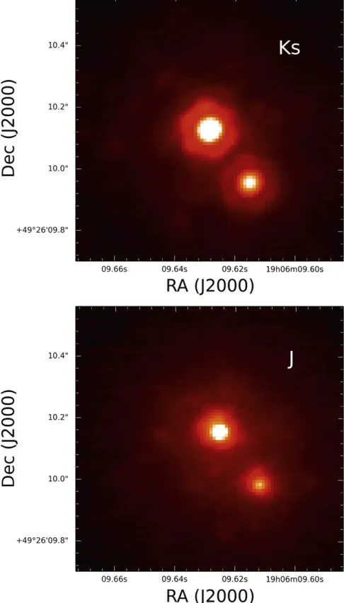
We observed Kepler-296 using the NIRC-2 instrument on the Keck II telescope using the Laser Guide Star Adaptive Optics system on 2013-08-08. We obtained a total integration time of 80 s with theKsfilter and 36 s inJband. As shown in Figure1, two stellar components are clearly resolved in the AO images. The flux ratio between the two stars in the J-band

image is 1.10±0.04 and in theKs-band image is 1.14±0.04

(brightnesses are shown in Table1).

Kepler-296 was observed as part of a campaign to obtain infrared spectra of cool Kepler Objects of Interest (KOIs)

(Muirhead et al.2012,2014). Muirhead et al. reported a stellar effective temperature,Teff =352070K, and an iron

abun-dance[Fe/H]=−0.08±0.14 dex.

We reanalyzed the spectrum from Muirhead et al. (2014) using the spectral fitting technique created by Covey et al.

(2010)and improved by Rojas-Ayala et al.(2012)but with a two spectrum modelfit applied to account for the two stars in the Kepler-296 system. This is a similar strategy to that employed and described by Montet et al.(2015). Specifically, we extract information on the temperature and metallicity of each star from observations of the Ks-band sodium doublet, calcium triplet, and absorption due to water opacity (the “

H O K22 - index”). In thefitting routine wefixed the ΔJ-band magnitude difference between the two stars to the values we measured using the NIRC-2 AO data. This analysis yielded temperatures for the two stars of 3435±58 and 3770±128 K and a surface gravity of 4.89±0.04 and 4.74±0.04 dex for the secondary and primary star, respectively.

When applying this method to combined-light spectra of two stars, there is a degeneracy between the allowed temperatures and metallicities of each star. Such degeneracy is reduced if we assume both stars have the same metallicity, as would be expected for a close binary pair. Assuming the stars are co-eval from the same cloud, we thenfit for one metallicty, measuring

[M/H] =−0.05±0.29. We note that the parameters found here are somewhat cooler than Cartier et al. (2015) who used

Hubble Space Telescope(HST)photometry to determine their

stellar properties. We have opted to use our values which are derived spectroscopically to the photometric properties pre-viously reported.

To estimate radii, densities, and theflux ratio of the two stars we used a grid of Dartmouth isochrones(Dotter et al. 2008). The grid is based on solar-scaled alpha-element abundances, and was interpolated to a step size of 0.01 Min mass and

0.02 dex metallicity using the interpolation tool provided in the Dartmouth database.14

We usedTeff,log g, and[Fe/H]of the primary to infer stellar properties from the isochrone grid using a Markov-Chain Monte-Carlo algorithm. We adopted uniform priors in mass, age, and metallicity. For ease of computation samples in age and metallicity were drawn in discrete steps corresponding to the sampling of the model grid(0.5 Gyr in age and 0.02 dex in

[Fe/H]). For each sample of fixed age and metallicity, we interpolated the grid in mass to deriveTeffandlog g, which are used to evaluate the likelihood function given the spectroscopic

Figure 1. NIRC-2 images of Kepler-296 inKsandJfilters show two stars separated by 0″. 217. The two images are scaled appropriately to account for differences in exposure time. The magnitude difference between the two stars is

J 1.10

D = andDKs=1.14.

Table 1

Summary of Properties Derived from AO Data

Property Primary Secondary

J 13.73±0.03 14.83±0.03

Ks 12.93±0.03 14.07±0.03

(J–Ks) 0.80±0.04 0.76±0.04

ΔR.A.(arcsec) L −0.130

Δdecl.(arcsec) L −0.174

q

D (arcsec) L 0.217

14

values forTeff,log g, and[Fe/H]. In addition toTeffandlog g, we interpolate in mass to derive absolute magnitudes in theKs

(MKs) and Kepler (MKp) bandpasses for the primary. For the

secondary, we added at each step the Ks contrast from AO imaging with a Gaussian random error to MKsderived for the primary and interpolated the grid in MKs to deriveTeff, mass,

g

log , and MKp for the secondary. Note that by fixing the secondary parameters to the primary we assume that both stars have the same age, metallicity, and distance.

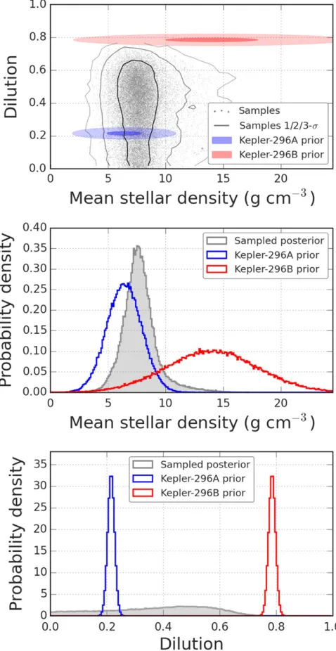
We calculated 106 iterations (discarding the first 10% as burn-in) and verified that the results are unaffected by the choice of initial guesses. The resulting MCMC chains provide stellar properties andKsandKeplerbandpass contrasts for both components (Table1). Figure2 shows both components in a Teff–density diagram as well as the stellar density posteriors and the derived dilution in the Kepler bandpass. The stellar properties we derive for both component stars are reported in Table2. We note that the properties for the secondary from the isochrone fit (Teff=345075K, log g 4.93 0.06

0.09

= -+ ) are in good agreement with the independent estimates from the spectroscopic analysis (Teff=343558K, log g

4.89 0.04

=  ).

Radii of interior models for cool stars are well known to show offsets from empirical observations such as long-baseline interferometry (Boyajian et al. 2012) or eclipsing binaries

(López-Morales2007; Irwin et al.2009). While recent models including magnetic field effects on convection show partial success to reproduce observations(Feiden & Chaboyer2013), empirical calibrations are commonly employed to avoid model-dependent offsets when estimating radii for cool planet host stars(Mann et al.2013). Using the most recentTeff- -R [Fe/H] relation from Mann et al. (2015)we derive empirical radii of 0.51Rfor Kepler-296 A and 0.35Rfor Kepler-296 B, which

are∼6%–9%(0.5 0.7s- )larger than the radii inferred from the isochrone grid. Importantly the fractional offsets are similar for both components and hence the densities of Kepler-296 A and B should not be strongly affected by differential model-dependent offsets.

Kepler has 4″pixels, therefore the two components, which

are separated by 0″. 217, are unresolved in theKeplerdata and can be treated as a point source. From our MCMC modeling we estimate a brightness difference in the Kepler bandpass of

ΔKp=1.41±0.08 which is equivalent to saying that 78.5± 1.2% of the light is coming from the primary and 21.5±1.2% from the secondary star in the binary. This is in good agreement with the results of Gilliland et al. (2015) and Cartier et al.

(2015)who reportHSTobservations that measure a brightness ratio of the two components of 5-to-1. Hereafter we define dilution as the proportion of total light coming from the other star, so the dilution of the primary star is 0.215±0.012.

Our analysis of the stellar properties relies on the two stars being physically bound. There are compelling arguments in previous work demonstrating that the two stars are highly likely to form a physically bound binary. Cartier et al.(2015)used model isochrones and performed a numerical analysis to show that the chances of observing two stars with these colors by chance is extremely unlikely. Similarly, Torres et al. (2015) look at the stellar density in this region of the sky where Kepler-296 is and used Galactic models to predict the chance alignment of an unbound star is very small compared with a bound companion scenario. In addition, if these stars were unbound this would likely result in two sets of stellar lines caused by differing radial velocities. However, Torres et al.

(2015)find no additional lines of another star appear in a Keck/ HIRES spectrum implying that the two stars have very similar radial velocities, as would be expected if they were bound.

3. KEPLERLIGHT CURVE MODELING

We modeled the long cadenceKepler data(Quintana et al. 2010; Twicken et al. 2010b) using a light curve model described by Rowe et al. (2014), Barclay et al. (2013), and Quintana et al. (2014)that comprises limb darkened transits

(Mandel & Agol2002)offive planet and allows the planets to have eccentric orbits. The parameters we use to describe the model are the mean density of the star, a linear and a quadratic limb darkening coefficient, a photometric zero-point, and for each planet, the mid-point of thefirst transit, the orbital period of the planet, the impact parameter at time of mid-transit, the planet-to-star radius ratio and two eccentricity vectorsesinw

andecoswwhereeis the eccentricity andωis the argument of the periastron. We also include an additional white noise term that is added in quadrature with the uncertainty reported in the

Keplerdata products. Finally, we include the dilution from the

other star as a model parameter.

Figure 2. Top panel: Dartmouth isochrones with an age of 6 Gyr and metallicities of-0.64,-0.34,-0.06, 0.22, and 0.48, roughly corresponding to the 2σerror bar from spectroscopy. The positions of Kepler-296A and B based on the median of the MCMC posteriors are shown as the red diamond and the blue triangle, respectively. Middle panel: posteriors for the density of both components. Bottom panel: posterior of the dilution in the Kepler

We used the Q1–Q15 Keplerlight curves. This target falls onto the failed Module 3 which resulted in no data for this source being taken in Quarters 8, 12, and 16. We used pre-search conditioned light curve data (Twicken et al. 2010a) which minimizes the instrumental signals. To remove astro-physical variability such as star spots we used a running medianfilter but weighted the transits zero in thisfiltering so as to avoid overly distorting the transit profiles.

We used emcee, an implementation of an affine invariant Markov Chain Monte Carlo algorithm (Goodman & Weare 2010; Foreman-Mackey et al. 2013) to efficiently explore the posterior probability of our transit model. We have made the assumption that all the planets orbit a single star but that star could either be Kepler-296A or Kepler-296B (for a discussion of the validity of this assumption see Section6). In the sampling we assumed uniform priors on the mean stellar density between 10−4 and 200 g cc−1 and a dilution, f, that is uniform between 0 and 1 where the total light from the system is unity and the light from the transited star is1-f.

We use uniform priors on the photometric zero point, the transit mid-point times, and the orbital period of the planets. The impact parameters are positive and uniform as is the planet-to-star radius ratio. Following Kipping(2013)we use a prior on the eccentricity of the orbits of the planets that takes the form of a beta distribution

P

B a b e e

1

( , ) (1 ) (1)

a 1 b 1

=

-b -

-where eis the orbital eccentricity of each planet andB is the beta function. Rowe et al. (2014) found that for multiple transiting planet systems the best fitting values for parameters

(a b, ) are a =0.4497 and b =1.7938 which we use in this work. In addition, we do not allow eccentricities that would allow for crossing orbits of any of the planets by excluding solutions where the periastron (or apastron)values are greater than(or less than)the semimajor axis of adjacent planets. We do, however, include a 1 e term in our likelihood function because our choice to sample in esinw and ecosw (rather thaneand ω)introduces a bias toward high values ofeif not modeled correctly (Eastman et al.2013).

Limb darkening is poorly constrained in the regime of cool stars(Claret et al.2012; Csizmadia et al.2013), so we assume a uniform distribution of the two limb darkening parameters but do enforce priors that keep the stellar brightness profile physical (Burke et al.2008).

In each simulation we used 800 chains with each chain taking 50,000 steps in the posterior probability. However, we discarded thefirst 10,000 steps in each chain for burn-in which leaves 32 M samples of the posterior probability.

4. MODEL COMPARISON

In our MCMC sampling we assumed uniform priors on stellar density and dilution. However, we are not ignorant of these parameters; indeed Section 2 describes our efforts to constrain these parameters. The reason for using uniform priors is that sampling from a bi-model parameter space which has well separated modes in a single model is difficult for standard MCMC algorithms (Kruschke 2014), while performing two MCMC simulations would necessitate computing the margin-alized likelihood which is a hard problem (Loredo1999).

We used a technique called importance sampling to re-sample the posterior under different priors than were used in the MCMC sampling. This is a well tested and used method when the posterior is difficult to sample directly (Hogg et al.2010).15Here we use importance sampling as a Bayesian evidence estimator. In this example we have two models, which we labelq1andq2, with two different sets of priors that contain our prior knowledge of the dilution and density for the planets orbiting the brighter star and the fainter star, respectively. Let α be the model we actually sampled from which is uniform in density and dilution. So we haveKsamples of(rk,fk)where

(

)

x

f p f p f p f

p

, ( , , ) ( , ) ( , )

( ) (2)

k k

r r a r a r

a

~ =

f

(r_k, _k) is drawn from p( ,r f∣x,a) where x is the observed data. Now what we want to compute is the marginalized likelihood of the data under modelsq1andq2, e.g.,

(

)

(

)

p qn =

ò

(

)

d df p ,d n p( , )f (4)

ò

=

wherep( ,r f∣qn)is the prior we want to enforce(qncan be either

1

q orq2)and is based on the measured densityrqand dilutionfq with uncertaintiesdr_q,df_q we calculated in Section2, such that

(

) (

)

(

)

p r,f qn =N r r dr; q, q N f f; q,dfq . (5)

Using the posterior samples from our MCMC sampling, we can approximate the integral as

(

)

(

)

(

)

(

)

(

) (

)

(

)

x x x

x x x x x x x

p d df p f p f p f

p f

p

d df p f p f

p f p f p f

p p K p f p f , ( , ) ( , , ) ( , , ) ( ) , , ( , ) ( , ) ( , , ) ( ) 1 , , , (6) n n n n k K

k k n

k k

1

ò

ò

å

q r r q r r a

r a

a

r r q r

r a r r a

q a r q r a = = ´ » =

which allows us to re-sample our data under the new priors. For a straight comparison betweenq1andq2, we can calculate

(

)

(

)

(

)

(

)

, . (7)

k K k k k K k k 1 2

1 1 1 1

1 2 2 2

q q r q r q » å å = =

In Figure 3 we show the sampling in dilution and mean stellar density under uniform priors in gray and the two different models,q1and q2 in blue and red, respectively. The blue model prior distribution overlaps significantly more with the sampled distribution than the red model, hinting that we are going to strongly prefer this model. We used Equation (7) under our modeling and foundp(x∣q1) p(x∣q2)=4713, that is

we are confident that the planets are orbiting the primary with a confidence level of 99.98%, provided all planets orbit the same star.

15

The reason why we are able to infer the planet’s host star is that the various transiting planet parameters are not entirely degenerate with dilution and stellar density. The key parameters that control the shape of the various transits are the stellar density which decreases with increasing transit duration, the planet-to-star radius ratio which increases with

transit depth, and the impact parameter which causes transits to be more “V”-shaped and decreases transit depths. So, for example, the transit can only be made so short by increasing the impact parameter before it becomes too V-shaped tofit the data: this limits the values stellar density can take.

5. REVISED PARAMETERS WITH THE PLANETS ORBITING THE PRIMARY

Given we are very confident that all the planets orbit the primary star (provided they all orbit the same star, this is discussed in detail in Section6), we can revise the stellar and

Figure 3.Sampled posterior probability based on theKeplerlight curve data and priors. The sampled posterior is shown in gray, the prior if thefive planets orbit 296A is shown in blue and the prior if the planets orbit Kepler-296B in red. The upper panel shows the joint-distribution of dilution and mean stellar density. The sampled data is shown as gray dots and the 1, 2, and 3-σ bounds of this sampling are shown as gray lines of decreasing opacity. The dark blue and red ellipses are the 1-σjoint distribution of the prior for Kepler-296 A and B respectively. The fainter blue and red ellipses are the 3-σbounds. Note that the sampling of the dilution-ρ distribution show negligible covariance. The central panel shows the mean stellar density marginal posterior distribution and the lower panel shows the dilution marginal posterior distribution. The Kepler-296A priors intuitively look more consistent with the observed Kepler light curve data than the Kepler-296B prior. We used importance sampling to quantify this intuition and we conclude with 99.9% probability that thefive planets orbit Kepler-296A.

planetary properties we calculated from our light curve modeling, properly accounting for the effect of dilution from the stellar companion. Given that a posterior probability is proportional to the product of the prior probability and the likelihood we can calculate the system’s parameters by weighting the original samples by the marginalized likelihood under the model of the planet orbiting Kepler-296 A where weights are equal to the probability p(x∣q)p(x∣a). In Table3 the weighted median and weighted quartiles are reported where a weighted median has 50% of the weight on either side. Figure 4 shows a transit model calculated using the MCMC sample with the highest weighted likelihood plotted over the phase-folded Kepler observations. In addition to the sampled parameters we report the ratio of the semi-major axis to the stellar radius (a Rs), the semi-major axis (a), the planetary radius (Rp), and the stellar flux incident on the planets (Sp). a Rsdepends only on stellar density and orbital period, whilea

and Rp rely on the stellar radius. We draw n stellar radii samples from the MCMC stellar property chains to properly include the stellar radius uncertainty and multiply these bya Rs and Rp Rsto infer aand Rp, wherenis the number of transit model samples.Spin solar-Earth units can be parametrized as a function ofa RsandTsso that

S S R

a a

R T

T (8)

p

s

2 s 4 =æ

è çç

çç ´

ö ø ÷÷÷ ÷

æ è ççç öø÷÷÷

Å Å

 

where SÅ is the incident flux on the Earth from the Sun,

a R

( Å )is the semi-major axis of the Earth in units of stellar

radius where we use 215.1 andT is the effective temperature

of the Sun which we have taken as 5778 K.

Thefive planets have radii of between 1.5 and 2.1RÅ, which places Kepler-296A into an elite group of planets with five small transiting planets that also includes Kepler-62(Borucki et al.2013), Kepler-186(Quintana et al.2014), and Kepler-444

(Campante et al. 2015). Kepler-296A is also one of just a handful of stars to host a sub-2 RÅ planet that receives less incidentflux than Earth receives from the Sun(Kepler-296 Af). Kepler-296 Ae and Af have been previously reported as potential habitable zone planets (Rowe et al. 2014; Torres et al.2015)—the region around a star where liquid water could exist given favorable atmospheric conditions. Kopparapu et al. (2013)published theoretical boundaries of incidentflux for circumstellar habitable zones; we find that Kepler-296 Ae falls into the Kopparapu et al.’s“optimistic”habitable zone and Kepler-296 Af in their “conservative”habitable zone.

Torres et al. (2015) model and report parameters for the outer two planets, the habitable zone planets, in the Kepler-296

Table 2

Derived Stellar Properties

Property Primary Secondary

Teff(K) 3740-+130130 3440-+7575

g

log (dex) 4.7740.059+0.091 4.933-+0.0630.087 [Fe/H] (dex) -0.08-+0.300.28 -0.08-+0.300.28

Radius(R) 0.480-+0.0870.066 0.322-+0.0680.060

Mass(M) 0.498-+0.0870.067 0.326-+0.0790.070 ρ(g cc−1) 6.4-+1.53.2 14-+48

ΔKp 0 1.409-+0.0700.085

Dilution 0.215±0.012 0.785±0.012

Table 3

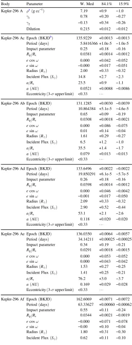
Inferred Stellar and Planetary Parameters from our MCMC Modeling

Body Parameter W. Med 84.1% 15.9%

Kepler-296 A ρa_{(g cc}−1_{) 7.19 +0.9 −1.0}

1

g 0.78 +0.20 −0.27

2

g −0.13 +0.34 −0.26

Dilution 0.215 +0.012 −0.012

Kepler-296 Ac Epoch(BKJDb) 135.9229 +0.0013 −0.0013 Period(days) 5.8416366 +1.0e-5 −1.0e-5 Impact parameter 0.25 +0.18 −0.16

R Rp s 0.0381 +0.0014 −0.0012

ecosw 0.000 +0.042 −0.052

esinw −0.000 +0.017 −0.051

Radius(RÅ) 2.00 +0.33 −0.32 Incident Flux(SÅ) 14.8 +2.7 −2.3

a Rs 23.5 +0.9 −1.1

a(AU) 0.0521 +0.0088 −0.0086

Eccentricity(3-σupper limit) <0.33 L

Kepler-296 Ab Epoch(BKJD) 131.1285 +0.0030 −0.0039 Period(days) 10.864384 +5.1e-5 −4.6e-5 Impact parameter 0.65 +0.09 −0.19

R Rp s 0.0308 +0.0018 −0.0021

ecosw 0.000 +0.086 −0.075

esinw 0.01 +0.14 −0.04

Radius(RÅ) 1.61 +0.29 −0.27 Incident Flux(SÅ) 6.5 +1.2 −1.0

a Rs 35.5 +1.4 −1.7

a(AU) 0.079 +0.013 −0.013

Eccentricity(3-σupper limit) <0.33 L

Kepler-296 Ad Epoch(BKJD) 133.6496 +0.0022 −0.0022 Period(days) 19.850291 +6.1e-5 −5.7e-5 Impact parameter 0.26 +0.18 −0.16

R Rp s 0.0398 +0.0014 −0.0012

ecosw 0.000 +0.046 −0.0042

esinw −0.001 +0.017 −0.050

Radius(RÅ) 2.09 +0.33 −0.32 Incident Flux(SÅ) 2.90 +0.52 −0.44

a Rs 53.1 +2.1 −2.6

a(AU) 0.118 +0.020 −0.020

Eccentricity(3-σupper limit) <0.33 L

Kepler-296 Ae Epoch(BKJD) 136.0350 +0.0064 −0.0057 Period(days) 34.14211 +0.00025−0.00025 Impact parameter 0.34 +0.19 −0.21

R Rp s 0.0291 +0.0018 −0.0015

ecosw 0.000 +0.053 −0.052

esinw 0.000 +0.043 −0.042

Radius(RÅ) 1.53 +0.27 −0.25 Incident Flux(SÅ) 1.41 +0.25 −0.21

a Rs 76.2 +3.0 −3.7

a(AU) 0.169 +0.029 −0.028

Eccentricity(3-σupper limit) <0.33 L

Kepler-296 Af Epoch(BKJD) 162.6069 +0.0071 −0.0072 Period(days) 63.33627 +0.00060−0.00062 Impact parameter 0.55 +0.11 −0.24

R Rp s 0.0344 +0.0021 −0.0019

ecosw −0.000 +0.071 −0.078

esinw −0.00 +0.10 −0.04

Radius(RÅ) 1.80 +0.31 −0.30

system. However, Torres et al. provide planet parameters for both stellar host scenarios. The planet parameters they report from their multi-modal nested sampling usingMULINEST(Feroz

& Hobson2008; Feroz et al. 2009)are largely consistent with our results if we consider only their model with planets orbiting the larger star. We see somewhat significant differences in Torres et al.’s derived planetary parameters. The discrepancy can be explained by the different stellar properties Torres et al. assume for the two stars compared with the analysis we present here. Torres et al. use spectroscopic parameters reported by Muirhead et al.(2014)who used just a single stellar spectrum model. By using two model spectra modeling we are able to improve upon previous stellar properties for both the stars in this system, removing the bias inherent when ignoring the companion.

6. THE VALIDITY OF OUR ASSUMPTION THAT THE PLANETS ORBIT THE SAME STAR

A critical assumption made in the analysis so far is that all

five planets orbit the same star. However, there is at least one example of a planetary system with planets orbiting different stellar members of the system—Kepler-132 (Lissauer et al. 2014). In the Kepler-132 system, two planets orbit one stellar companion of a binary while one planet orbits its companion. As a result, it is important that we assess whether our assumption that the planets all orbit the same star is justified.

In order for the planets to orbit different stars, and yet be seen in transit, the orbital planes of the two planetary systems must nearly line up (their angular momentum vectors must point in nearly the same direction).

In approximate terms, the difference in angle between the two orbital planes(of the two putative planetary systems)must be less than the alignment necessary for the planets to transit, i.e.,

R

a

R

* 0.3

0.2 AU 0.0070 rad 0 . 4, (9) P

 q

D ~  ~ ~ ◦

where we have used the small angle approximation. In other words, the required alignment is extremely tight, with a tolerance of less than half a degree. The binary has a projected

separation of about 35 AU, so the question becomes: What is the probability that nature will produce two planetary systems around the two binary components separated by at least 35 AU, such that the orbital angular momenta point in the same direction(within0 . 5◦ )?

6.1. Considerations of Disk Formation

Molecular cloud cores are the sites of star formation and their angular momentum profiles drive the formation of the circumstellar disks(which, in turn, provides the sites for planet formation). The rotation rate of these cores is estimated by measuring the velocity gradient of a given molecular line across a map of the core(starting with Goodman et al.1993). However, the direction of the inferred (two-dimensional) angular momentum vector varies from point to point within the map (Caselli et al.2002). As a result, the mean velocity gradients have values of~ -1 2km s−1pc−1, but the direction of the rotation varies by 10°–30°across the map. Moreover, the emission maps show a coherence length ofℓ»0.01pc, i.e., for two points separated by distances larger thanℓ, the directions of the rotation vectors are uncorrelated. Here, “uncorrelated” means chosen randomly from the distribution of values within the measured range, where the measured range is of order 30°.

(Note that the range is not 360°; if that were the case, the rotation vectors would take on a purely random direction for points separated by distances greater thanℓ.)

We can build a simple model of star/binary/disk formation using the results given above. As a first approximation, consider the density profile of the initial molecular cloud core to have the isothermal form

a

Gr

2 , (10)

2

2

r p

= L

where a is the isothermal sound speed and L ~ -1 2 is the overdensity factor (Fatuzzo et al. 2004)that accounts for the observed condensation velocities (Lee et al. 1999). The corresponding enclosed mass is thus given by

M r a

G r

( ) 2 . (11)

2 = L

The radiusrPthat initial encloses the massMPof the primary can be written in the form

r GM

a

M

M

a

2 3 10 cm 0.33 0.20 km s .

(12)

P P P

2

16

1 2 =

L » ´

æ è çç çç

ö ø ÷÷÷ ÷ æ è

ççç - öø÷÷÷

-

We thus note thatrp~ ~ℓ 0.01pc, i.e., the sphere that initially

contained the mass of the primary is comparable to the coherence length observed in molecular cloud cores. As a result, the primary, and the inner disk that forms its planetary system, can have a different direction for its angular momentum vector than the material that collapses later to form the secondary. Further, we would expect that the angle between the angular momenta of these different layers of the core to be tens of degrees. With this type of initial condition, the direction of the orbit of the binary companion is predicted to differ from that of the planetary system by tens of degrees

(also see Spalding et al.2014).

Table 3 (Continued)

Body Parameter W. Med 84.1% 15.9%

a Rs 115.1 +4.5 −5.6

a(AU) 0.255 +0.043 −0.042

Eccentricity(3-σupper limit) <0.33 L

Notes.Parameters are the weighted quartiles of the posterior distribution where the weights were calculated via importance sampling.

a

The stellar radius and stellar mass for Kepler-296A are listed in Table1and are R=0.4800.076, and R=0.4980.076. The stellar mass and

radius are not strictly consistent with the density present here because this density was calculated using additional information from the transit model.

b

The time zeropoint we use id the Barycentric Julian Date minus afixed offset of 2454833 days. This is referred to as BKJD and is the time system used in all

As a consistency check, consider the centrifugal radius produced during the collapse. When the inner portion of the core has collapsed to form the primary, the centrifugal radius

R G M

a

16 2 20 AU. (13)

P

C

3 3 2

3 8

= W

L »

-As a result, the primary and its planetary system, whose size is determined by RCto leading order, canfit inside the observed binary orbital separation of the Kepler-296 system(which has a projected separation of 35 AU and hence expected separation of about 70 AU).

This simple theoretical argument predicts that the disks observed in binary systems should not be perfectly aligned with the angular momentum vectors of the binary orbits and that the disks surrounding the two stars should not be aligned with each other. Since disks polarize the light scattered from their central stars, polarization measurements can be used to estimate the angular orientation of disks on the plane of the sky. Such a study has been carried out for a collection of 19 binary and higher-order multiple T Tauri systems(Jensen et al.2004); the results show that disks in binary systems are aligned with each other to within about 20, but are not exactly coplanar. A similar study for southern star formation regions (Monin et al. 2006) finds similar results; for 15 binary systems, the observed angle differences show a distribution of values, with all but one in the range 0°–40°, and more than half of the sources showing relatively small anglesD <q 10.

Both the theoretical argument and the observational studies indicate that two planetary systems associated with the two members of a binary pair should be roughly—but not exactly— aligned. The range of possible relative orientation angles appears to be about 20 . We can thus make a simple estimate of the probability to find highly aligned planetary systems: if the relative inclination angle is drawn uniformly from the range

20 q 20

-  < D < , and if we need ∣Dq∣<0 . 5◦ to observe transits, then the required alignment would occur only about 1 out of 40 times (2.5%).

6.2. Probability

This subsection considers a simple probability argument: the

five periods of the planets are observed to be almost equally spaced in a logarithmic sense: the period ratios between successive pairs of planets are all ∼1.8(more precisely, 1.88, 1.83, 1.71, and 1.86, with a mean of 1.82±0.066). This chain of nearly equal period ratios can naturally be produced if the planets experienced convergent migration during their early stages of evolution. On the other hand, if one or more planets orbit the secondary (with the rest of the planets orbiting the primary), then this set of nearly equal period ratios would be highly unlikely.

We can understand (roughly) how convergent migration results in regular orbital spacing as follows: when multiple planets migrate within a disk, they often lock into mean motion resonance (MMR) and move inward together (this phenom-enon has been studied by many authors, starting with Goldreich 1965). Indeed, since orbital eccentricity is easily excited during migration, the planets must often be in, or near, MMR to avoid orbit crossing and instability. The most common and strongest resonances in this context are the 2:1 and 3:2 MMR (Murray & Dermott 1999). With these period ratios, the semimajor axes of the planets are separated by

factors of f » 1.59 and 1.31, respectively, so that orbital spacings in this range are naturally produced. Moreover, detailed numerical studies(Rein2012)indicate that the period ratios for the multiplanet systems discovered by Kepler are indeed consistent with convergent planet migration. Additional stochastic forces(e.g., due to turbulentfluctuations in the disk) act to spread out the orbital spacing (Adams et al. 2008), so that values in the range 1.3–2 are naturally produced(including the value of 1.8 observed for Kepler-296).

If thefive planets detected in association with Kepler-296 do not orbit the same star, then there should be no correlation(or anti-correlation) between the orbital periods of the planets orbiting the two different stars. Since there are many possible ways for this scenario to be realized, we illustrate this point here by assuming that one planet orbits the secondary, while the other four planets orbit the primary. The period of the secondary planet should be independent of the periods of the four primary planets, so there is some chance that the secondary planetary period would be close to one of the periods of the others—close enough to render the system apparently unstable if one mistakenly considered all of the planets to orbit a single star.

To make a numerical estimate, suppose that the orbital periods are distributed with a log-random distribution. The observed planets have periods with a spacing of ∼1.8 (as described above). However, if a planetary pair were to have a period ratio that is too close to unity, it would most likely be unstable (in the absence of a well-tuned resonant state). As a general rule, orbital instability sets in when the semi-major axes are too close, more specifically when their separation is less than several mutual Hill radii. In practice, however, we find that theKeplermulti-planet systems have extremely few period ratios less than 4:3, i.e., the period ratio is almost never observed to be less than 4/3=1.33.

Suppose we have a chain of planets with a factor of 1.8 spacing in period and we choose another planet from a log-random distribution. Then the chances of the new planet being too close to another planet in the chain is given approximately by the expression

P ln(4 3)

ln(1.8) 0.49. (14)

= »

In other words, about 49% of the time, if you choose a planet around the secondary, it would have a period that is too close to one of the other planets (orbiting the primary), such that it would apparently lead to an unstable system.

ratios is approximately given by

P ln(1.886 1.754)

ln(11) 0.030. (15)

» »

In other words, the probability of continuing the observed chain of orbital period ratios is about 3% (and this value would be smaller if we allowed for a wider range of orbits to choose from).

6.3. Discussion of Planetary Alignment

The two arguments given above suggest that two highly aligned planetary systems orbiting the two members of a binary pair will be rare. More specifically, the chances of forming such a system(Section6.1)and the chances that planets orbiting two stars produce a coherent chain of period ratios(Section6.2)are both approximately2% 3%- .

Either argument, by itself, is highly suggestive but not definitive. With a 3% occurrence rate, if we observe∼35 binary systems containing multiple transiting planets, then we would expect tofind sufficient alignment in(of order)one system. In this case, however, the two arguments are independent. We need to see thefive planets of the Kepler-296 system in transit

(a 2.5% effect)and also see the observed chain of period ratios

(another 3% effect). The chances of both properties occurring is thus much lower, with a probability P~(0.025)(0.03) = 7.5_´10-4_{. With this probability, we would need to observe} more than 1300 binary systems with multiple planets in order to expect one with these properties.

In the most recent release ofKeplerplanet candidates, there are 608 multiple transiting planet systems comprising 1492 planet candidates(Mullally et al.2015). Of those systems, only Kepler-132 presents a compelling case for a binary star with transiting planets orbiting both stars. The planets in the Kepler-132 system are on considerably shorter periods(6.1, 6.4, and 18 days)and orbit a star more than twice the size of the planets in the Kepler-296 system, hence the probability of the observed planets to transit Kepler-132 is much higher. The probability to transit Kepler-132c and d is roughly 8% and 4%, respectively, whereas the probability for Kepler-296Ae and f to transit is roughly 1.3% and 0.9%, respectively. Therefore, it is many times more probable that two stars have disks aligned enough for transiting planets in the Kepler-132 system than in the Kepler-296 system. Indeed, we should not be surprised to see a false positive case occurring for close-in two-planet systems.

Perhaps a fairer family to compare Kepler-296 to is a system with at leastfive transiting planets. Of the 608 multi-transiting planet systems just 24 host at least 5 planet candidates, inclusive of Kepler-296. At most 50% of these five planet systems are likely to be binaries(Wang et al.2014). Taking the false positive rate for systems like Kepler-296 as 7.5_´10-4 and having(0.5 × 24)systems, we would expect to see 0.009 false multi-systems, making it very likely that the planets in the Kepler-296 system orbit the same star. This result validates the assumptions made in earlier sections and leads us to the conclusion that the five planets orbit Kepler-296A.

7. NOMENCLATURE

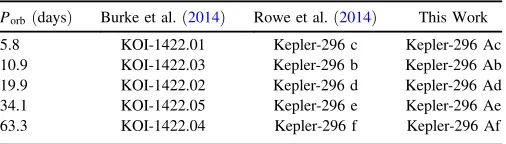
We want to briefly touch upon our naming system for the planets in this system. The five planets have KOI numbers 1422.01, 1422.03, KOI-1422.02, KOI-1422.05, and KOI-1422.04 in order of increasing orbital period. Owing to

the additional data available to us in this work compared to that used by Rowe et al. (2014) and Lissauer et al. (2014), we realized that KOI-1422.03 had an orbital period of 10.86 days, a factor of precisely three longer than was reported by Rowe et al. (2014) and Lissauer et al. (2014) who assigned the Kepler number 296 to this system. To retain consistency with Rowe et al. (2014) we stick with the letter b to identify KOI-1422.03 even though planet b now has a longer orbital period than planet c. We note that recent Kepler planet candidate catalogs all list KOI-1422.03 with an orbital period of 10.86 days(Burke et al.2014; Mullally et al. 2015; Rowe et al.2015). In addition, Torres et al.(2015)used 10.86 days as the orbital period of KOI-1422.03 in their analysis of the stellar density (G. Torres & D. Kipping 2015, private communica-tion). All papers subsequent to the earlier discovery papersfind an orbital period of 10.86 days and we believe that it is highly probable that this is the correct orbital period solution.

In our naming scheme we also use the letter A after the primary star name to make it clear that the planets orbit the primary star in the binary. Consequently, identifiers now used for these planets, in order of increasing orbital period are Kepler-296 Ac, Kepler-296 Ab, Kepler-296 Ad, Kepler-296 Ae and Kepler-296 Af. We summarize this information in Table4.

8. CONCLUSIONS

The Galaxy is expected to contain many binary systems with planets orbiting one or both stellar components. In this work, we have explored whether it is likely that one will observe planets (in multi-planet systems) transiting both stellar components. For the solar system architecture of the Kepler-296 system, this exploration strongly indicates that allfive of the observed planets are likley to orbit the primary.

The paper presents a statistical analysis which demonstrates that if the planets all orbit the same star, then that host star must be the brighter component of the binary system. For this analysis, we start by modeling theKeplerlight curve of Kepler-296 under a prior with no preference for stellar properties(see Section3). We then compare the two competing models of(a) planets orbiting the brighter star or (b) planets orbiting the fainter star, where the comparison uses importance sampling under the different priors(Section4). Wefind that the planets are significantly more likely to orbit the brighter star.

The paper also provides a supporting statistical argument for the orbital alignment of high multiplicity transiting planet systems such as Kepler-296. This analysis(Section6)indicates that it is highly unlikely that one would observe planets transiting both stars—where the odds are less than about 1 in 1000 for this example. The reason for this low probability of observing planets in transit orbiting both stars is twofold:(a) the probability of randomly observing a system with planets orbiting both stars such that the system is apparently stable and the planets are in an apparent(near) resonant chain is only a

Table 4

Nomenclature for the Kepler-296 A Planets

Porb(days) Burke et al.(2014) Rowe et al.(2014) This Work

few percent, and (b) the probability of having the two stars with aligned circumstellar disks is also only a few percent. The probability of realizingbothof these independent and unlikely events occurring is thus low.

The combination of the two analyses described above provides a compelling argument that the currently observed planets in the Kepler-296 system must orbit the brighter star. With thisfinding taken as given, the planetary properties can be determined to greater precision than before. This paper thus reports revised estimates for the planetary radii, orbital periods, and incident stellar fluxes for the outer planets in the system Kepler-296 Ae and Kepler-296 Af(see Section5). This update to the planetary parameters is important as these planets are thought to orbit within or near the habitable zone (see also Torres et al. 2015) of their host star (argued here to be the primary, Kepler-296A). After the first discovery of the first Earth-sized planet in the habitable zone(Quintana et al.2014), and a dozen subsequent detections (Torres et al. 2015), we expect the Galaxy to be brimming with analogous planets. The discovery and characterization of such planetary systems thus poses a rich problem for future work.

This paper includes data collected by the Kepler mission. Funding for the Kepler mission is provided by the NASA Science Mission Directorate. We would like to express our gratitude to all those who have worked on theKeplerpipeline over the many years of the Keplermission. SomeKeplerdata presented in this paper were obtained from the Mikulski Archive for Space Telescopes(MAST)at the Space Telescope Science Institute(STScI). STScI is operated by the Association of Universities for Research in Astronomy, Inc., under NASA contract NAS5-26555. Support for MAST for non-HSTdata is provided by the NASA Office of Space Science via grant NNX09AF08G and by other grants and contracts. This research has made use of the NASA Exoplanet Archive, which is operated by the California Institute of Technology, under contract with the National Aeronautics and Space Administra-tion under the Exoplanet ExploraAdministra-tion Program. This research made use of APLpy, an open-source plotting package for Python hosted athttp://aplpy.github.com. This work was supported by a NASA Keck PI Data Award, administered by the NASA Exoplanet Science Institute. Some of the data presented herein were obtained at the W. M. Keck Observatory from telescope time allocated to the National Aeronautics and Space Administration through the agency’s scientific partner-ship with the California Institute of Technology and the University of California. The Observatory was made possible by the generous financial support of the W. M. Keck Foundation. The authors wish to recognize and acknowledge the very significant cultural role and reverence that the summit of Maunakea has always had within the indigenous Hawaiian community. We are most fortunate to have the opportunity to conduct observations from this mountain. E.V.Q. is supported by a NASA Senior Fellowship at the Ames Research Center, administered by Oak Ridge Associated Universities through a contract with NASA. B.T.M. is supported by the National Science Foundation Graduate Research Fellowship under Grant No. DGE1144469. D.H. acknowledges support by the Australian Research Council’s Discovery Projects funding scheme (project number DE140101364) and support by the National Aeronautics and Space Administration under Grant

NNX14AB92G issued through the Kepler Participating Scientist Program.

REFERENCES

Adams, F. C., Laughlin, G., & Bloch, A. M. 2008,ApJ,683, 1117 Barclay, T., Burke, C. J., Howell, S. B., et al. 2013,ApJ,768, 101 Batalha, N. M., Rowe, J. F., Bryson, S. T., et al. 2013,ApJS,204, 24 Borucki, W. J., Agol, E., Fressin, F., et al. 2013,Sci,340, 587 Boyajian, T. S., von Braun, K., van Belle, G., et al. 2012,ApJ,757, 112 Burke, C. J., Bryson, S. T., Mullally, F., et al. 2014,ApJS,210, 19 Burke, C. J., McCullough, P. R., Valenti, J. A., et al. 2008,ApJ,686, 1331 Cameron, E., & Pettitt, T. 2013, arXiv:1309.2737

Campante, T. L., Barclay, T., Swift, J. J., et al. 2015,ApJ,799, 170 Cartier, K. M. S., Gilliland, R. L., Wright, J. T., & Ciardi, D. R. 2015,ApJ,804, 97 Caselli, P., Benson, P. J., Myers, P. C., & Tafalla, M. 2002,ApJ,572, 238 Claret, A., Hauschildt, P. H., & Witte, S. 2012,A&A,546, A14

Covey, K. R., Lada, C. J., Román-Zúñiga, C., et al. 2010,ApJ,722, 971 Csizmadia, S., Pasternacki, T., Dreyer, C., et al. 2013,A&A,549, A9 Dotter, A., Chaboyer, B., Jevremović, D., et al. 2008,ApJS,178, 89 Duquennoy, A., & Mayor, M. 1991, A&A,248, 485

Eastman, J., Gaudi, B. S., & Agol, E. 2013,PASP,125, 83 Fatuzzo, M., Adams, F. C., & Myers, P. C. 2004,ApJ,615, 813 Feiden, G. A., & Chaboyer, B. 2013,ApJ,779, 183

Feroz, F., & Hobson, M. P. 2008,MNRAS,384, 449

Feroz, F., Hobson, M. P., & Bridges, M. 2009,MNRAS,398, 1601 Foreman-Mackey, D., Hogg, D. W., Lang, D., & Goodman, J. 2013,PASP,

125, 306

Gilliland, R. L., Cartier, K. M. S., Adams, E. R., et al. 2015,AJ,149, 24 Gilliland, R. L., Marcy, G. W., Rowe, J. F., et al. 2013,ApJ,766, 40 Goldreich, P. 1965,MNRAS,130, 159

Goodman, A. A., Benson, P. J., Fuller, G. A., & Myers, P. C. 1993,ApJ, 406, 528

Goodman, J., & Weare, J. 2010,Comm. App. Math. Comp. Sci,5, 65 Hogg, D. W., Myers, A. D., & Bovy, J. 2010,ApJ,725, 2166

Horch, E. P., Howell, S. B., Everett, M. E., & Ciardi, D. R. 2012,AJ,144, 165 Horch, E. P., Howell, S. B., Everett, M. E., & Ciardi, D. R. 2014,ApJ,795, 60 Irwin, J., Charbonneau, D., Berta, Z. K., et al. 2009,ApJ,701, 1436 Jensen, E. L. N., Mathieu, R. D., Donar, A. X., & Dullighan, A. 2004,ApJ,

600, 789

Kipping, D. M. 2013,MNRAS,434, L51

Kopparapu, R. K., Ramirez, R., Kasting, J. F., et al. 2013,ApJ,765, 131 Kruschke, J. K. 2014, in Doing Bayesian Data Analysis: A Tutorial with R,

JAGS, and Stan(2nd ed; New York: Academic Press) Lee, C. W., Myers, P. C., & Tafalla, M. 1999,ApJ,526, 788 Lissauer, J. J., Marcy, G. W., Bryson, S. T., et al. 2014,ApJ,784, 44 López-Morales, M. 2007,ApJ,660, 732

Loredo, T. J. 1999, in ASP Conf. Ser. 172, Astronomical Data Analysis Software and Systems VIII, ed. D. M. Mehringer, R. L. Plante & D. A. Roberts(San Francisco, CA: ASP), 297

Mandel, K., & Agol, E. 2002,ApJL,580, L171

Mann, A. W., Feiden, G. A., Gaidos, E., & Boyajian, T. 2015,ApJ,804, 64 Mann, A. W., Gaidos, E., & Ansdell, M. 2013,ApJ,779, 188

Monin, J.-L., Ménard, F., & Peretto, N. 2006,A&A,446, 201

Montet, B. T., Johnson, J. A., Muirhead, P. S., et al. 2015,ApJ,800, 134 Muirhead, P. S., Becker, J., Feiden, G. A., et al. 2014,ApJS,213, 5 Muirhead, P. S., Hamren, K., Schlawin, E., et al. 2012,ApJL,750, L37 Mullally, F., Coughlin, J. L., Thompson, S. E., et al. 2015,ApJS,217, 31 Murray, C. D., & Dermott, S. F. 1999, in Solar System Dynamics(Cambridge:

Cambridge Univ. Press)

Quintana, E. V., Barclay, T., Raymond, S. N., et al. 2014,Sci,344, 277 Quintana, E. V., Jenkins, J. M., Clarke, B. D., et al. 2010,Proc. SPIE,7740,

77401X

Raghavan, D., McAlister, H. A., Henry, T. J., et al. 2010,ApJS,190, 1 Rein, H. 2012, MNRAS,427, L21

Rojas-Ayala, B., Covey, K. R., Muirhead, P. S., & Lloyd, J. P. 2012,ApJ, 748, 93

Rowe, J. F., Bryson, S. T., Marcy, G. W., et al. 2014,ApJ,784, 45 Rowe, J. F., Coughlin, J. L., Antoci, V., et al. 2015,ApJS,217, 16 Spalding, C., Batygin, K., & Adams, F. C. 2014,ApJL,797, L29 Tenenbaum, P., Jenkins, J. M., Seader, S., et al. 2013,ApJS,206, 5 Tenenbaum, P., Jenkins, J. M., Seader, S., et al. 2014,ApJS,211, 6 Torres, G., Kipping, D. M., Fressin, F., et al. 2015,ApJ,800, 99

Twicken, J. D., Chandrasekaran, H., Jenkins, J. M., et al. 2010,Proc. SPIE, 7740, 774023

Twicken, J. D., Clarke, B. D., Bryson, S. T., et al. 2010,Proc. SPIE,7740, 77401U