This is a repository copy of Nonlinear output frequency response functions for multi-input
nonlinear volterra systems.
White Rose Research Online URL for this paper: http://eprints.whiterose.ac.uk/74574/
Monograph:
Peng, Z.K., Lang, Z.Q. and Billings, S.A. (2006) Nonlinear output frequency response functions for multi-input nonlinear volterra systems. Research Report. ACSE Research Report no. 925 . Automatic Control and Systems Engineering, University of Sheffield
eprints@whiterose.ac.uk https://eprints.whiterose.ac.uk/
Reuse
Unless indicated otherwise, fulltext items are protected by copyright with all rights reserved. The copyright exception in section 29 of the Copyright, Designs and Patents Act 1988 allows the making of a single copy solely for the purpose of non-commercial research or private study within the limits of fair dealing. The publisher or other rights-holder may allow further reproduction and re-use of this version - refer to the White Rose Research Online record for this item. Where records identify the publisher as the copyright holder, users can verify any specific terms of use on the publisher’s website.
Takedown
If you consider content in White Rose Research Online to be in breach of UK law, please notify us by
Nonlinear Output Frequency Response Functions for
Multi-Input Nonlinear Volterra Systems
Z K Peng, Z Q Lang, and S A Billings
Department of Automatic Control and Systems Engineering The University of Sheffield
Mappin Street, Sheffield S1 3JD, UK
Nonlinear Output Frequency Response Functions
for Multi-Input Nonlinear Volterra Systems
Z.K. Peng, Z.Q. Lang, and S. A. Billings
Department of Automatic Control and Systems Engineering, University of Sheffield
Mappin Street, Sheffield, S1 3JD, UK
Email: z.peng@sheffield.ac.uk; z.lang@sheffield.ac.uk; s.billings@sheffield.ac.uk
Abstract: The concept of Nonlinear Output Frequency Response Functions (NOFRFs) is extended to the nonlinear systems that can be described by a multi-input Volterra series
model. A new algorithm is also developed to determine the output frequency range of
nonlinear systems from the frequency range of the inputs. These results allow the concept
of NOFRFs to be applied to a wide range of engineering systems. The phenomenon of the
energy transfer in a two degree of freedom nonlinear system is studied using the new
concepts to demonstrate the significance of the new results.
1 Introduction
Linear systems, which have been widely studied by practitioners in many different fields,
have provided a basis for the development of the majority of control system synthesis,
mechanical system analysis and design, and signal processing methods. However, there
are certain types of qualitative behaviour encountered in engineering, which cannot be
produced by linear models [1], for example, the generation of harmonics and inter-
modulation behaviour. In cases where these effects are dominant or significant nonlinear
behaviours exist, nonlinear models are required to describe the system, and nonlinear
system analysis methods have to be applied to investigate the system dynamics.
The Volterra series approach [2] is a powerful tool for the analysis of nonlinear systems,
which extends the familiar concept of the convolution integral for linear systems to a
series of multi-dimensional convolution integrals. The Fourier transforms of the Volterra
kernels are known as the kernel transforms, Higher-order Frequency Response Functions
(HFRFs) [3], or Generalised Frequency Response Functions (GFRFs), and these provide
a convenient tool for analyzing nonlinear systems in the frequency domain. If a
differential equation or discrete-time model is available for a system, the GFRFs can be
determined using the algorithm in [4]~[6]. The GFRFs can be regarded as the extension
However, the GFRFs are much more complicated than the FRF. GFRFs are
multidimensional functions [7][8], which can be difficult to measure, display and
interpret in practice. Recently, the novel concept of Nonlinear Output Frequency
Response Functions (NOFRFs) was proposed by the authors [9]. The concept can be
considered to be an alternative extension of the FRF to the nonlinear case. NOFRFs are
one dimensional functions of frequency, which allow the analysis of nonlinear systems to
be implemented in a manner similar to the analysis of linear systems and which provides
great insight into the mechanisms which dominate many nonlinear behaviours. The
NOFRF concept was recently used to investigate the energy transfer properties of bilinear
oscillators in the frequency domain [10]. The results revealed the existence of resonances
at frequencies different from the frequencies at the input excitation in this class of
oscillators.
The objective of this paper is to extend the concept of NOFRFs to multi-input nonlinear
Volterra systems so that the concept of NOFRFs can be applied to a much wider range of
engineering systems. The phenomenon of energy transfer in a 2DOF nonlinear system is
also investigated using the extended concept of NOFRFs to demonstrate the effectiveness
and significance of the results obtained in the present study.
2 The Concept of Nonlinear Output Frequency Response Functions
NOFRFs were recently proposed and used to investigate the behaviour of structures with
polynomial-type non-linearities. The definition of NOFRFs is based on the Volterra
series theory of nonlinear systems.
Consider the class of nonlinear systems which are stable at zero equilibrium and which
can be described in the neighbourhood of the equilibrium by the Volterra series
i n
i
i n
N
n
n x t d
h t
y( ) (τ ,...,τ ) ( τ ) τ 1
1
1
∏
∑∫ ∫
= =
∞ ∞ −
∞ ∞
− −
= L (1.1)
where y(t) and x(t) are the output and input of the system, hn(τ1,...,τn) is the nth order
Volterra kernel, and N denotes the maximum order of the system nonlinearity. Lang and
Billings [3] have derived an expression for the output frequency response of this class of
nonlinear systems to a general input. The result is
⎪ ⎪ ⎩ ⎪ ⎪ ⎨ ⎧
=
∀ =
∫
∏
∑
= +
+ =
− =
ω ω ω
ω σ ω ω
ω π
ω
ω ω
ω
n
n n
i
i n
n n
n
N
n n
d j X j
j H n
j Y
j Y j
Y
,..., 1
1 1
1
1
) ( ) ,..., ( )
2 (
1 ) (
for
) ( )
(
This expression reveals how nonlinear mechanisms operate on the input spectra to
produce the system output frequency response. In (1.2), Y(jω) and X(jω)are the spectra
of the system output and input respectively, Yn(jω) represents the nth order output
frequency response of the system,
n j
n n
n
n j j h e d d
H ( ω ,..., ω ) ... (τ ,...,τ ) ωτ ωnτn τ ... τ 1 ) ,..., ( 1
1
1 1 + +
− ∞
∞ − ∞
∞ −
∫
∫
= (1.3)
is the definition of the Generalised Frequency Response Function (GFRF), and
∫
∏
= +
+ ω ω =
ω
ω
σ ω ω
ω n
n n
i
i n
n j j X j d
H
,..., 1
1
1
) ( ) ,..., (
denotes the integration of
∏
over the n-dimensional hyper-plane =n
i
i n
n j j X j
H
1
1,..., ) ( )
( ω ω ω
ω ω
ω1+L+ n = . Equation (1.2) is a natural extension of the well-known linear relationship Y(jω)=H1(jω)X(jω) to the nonlinear case.
For linear systems, the possible output frequencies are the same as the frequencies in the
input. For nonlinear systems described by Equation (1.1), however, the relationship
between the input and output frequencies is more complicated. Given the frequency range
of the input, the output frequencies of system (1.1) can be determined using an explicit
expression derived by Lang and Billings in [3].
Based on the above results for output frequency responses of nonlinear systems, a new
concept known as the Nonlinear Output Frequency Response Function (NOFRF) was
recently introduced by Lang and Billings [9]. The concept was defined as
∫ ∏
∫
∏
= +
+ =
= +
+ =
=
ω ω ω
ω ω
ω ω
ω
σ ω
σ ω ω
ω ω
n n
n n
i
i
n n
i
i n
n n
d j X
d j X j
j H j
G
,..., 1
,..., 1
1
1 1
) (
) ( ) ,..., ( )
( (1.4)
under the condition that
0 )
( )
(
,..., 1
1
≠
=
∫ ∏
= + + ω ω =
ω
ω
σ ω ω
n
n n
i
i
n j X j d
U (1.5)
Notice that Gn(jω) is valid over the frequency range of Un(jω) , which can be
determined using the algorithm in [3].
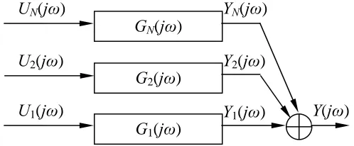
By introducing the NOFRFs Gn(jω), n=1,LN, Equation (1.4) can be written as
∑
∑
= =
=
= N
n
n n
N
n
n j G j U j
Y j
Y
1 1
) ( ) ( )
( )
( ω ω ω ω (1.6)
which is similar to the description of the output frequency response of linear systems. For
Figure 1. Similarly, the nonlinear system input and output relationship of Equation (1.1)
[image:6.612.177.426.173.276.2]can be illustrated in Figure 2.
Figure 1. The output frequency response of a linear system
Figure 2. The output frequency response of a nonlinear system
The NOFRFs reflect a combined contribution of the system and the input to the
frequency domain output behaviour. It can be seen from Equation (1.4) that Gn(jω)
depends not only on Hn (i=1,…,N) but also on the input X(jω). For a nonlinear system,
the dynamical properties are determined by the GFRFs (i= 1,…,N). However, from
Equation (1.3) it can be seen that a GFRF is multidimensional [7][8], and may become
difficult to measure, display and interpret in practice. Feijoo, Worden and Stanway
[11]-[12] demonstrated that the Volterra series can be described by a series of associated linear
equations (ALEs) whose corresponding associated frequency response functions (AFRFs)
are easier to analyze and interpret than the GFRFs. According to Equation (1.4), the
NOFRF
n H
) (jω
Gn is a weighted sum of Hn(jω1,...,jωn) over ω1+L+ωn =ω with the weights depending on the input. Therefore Gn(jω) can be used as an alternative
representation of the structural dynamical characteristics described by . The most
important property of the NOFRF
n H
) (jω
Gn is that it is one dimensional, and thus allows
the analysis of nonlinear systems to be implemented in a convenient manner similar to
the analysis of linear systems. Moreover, there is an effective algorithm [9] available
which allows the evaluation of the NOFRFs to be implemented directly using system
input output data.
2 NOFRFS for Multi-Input Nonlinear Volterra Systems
2.1 Multi-Input Nonlinear Volterra Systems
Multi-input multi-output nonlinear Volterra systems can be expressed so that each output
can to be modeled as a multi-input Volterra series. The extension of the single input
single output Volterra series representation (1.1) to this more general case is as follows UN(j )
U2(j )
U1(j ) Y1(j )
Y2(j )
YN(j )
G1(j )
G2(j )
GN(j )
Y(j )
X(j ) Y(j )
∑
= = N n n i i t y t y 1 ) ( ) ( )( (2.1)
where n n m N N m N N N n N N N n n N P N P i n i d d t x t x t x t x t x t x h t y m m m m τ τ τ τ τ τ τ τ τ τ L L L L L L L L L L 1 1 2 1 2 1 1 1 1 ) ( ) , , , ( ) ( ) ( ) ( ) ( ) ( ) ( ) ( ) , , ( ) ( 1 1 2 1 1 1 1 1 1 − − − − − − = + + + + + = + + +∞ ∞ − +∞ ∞ − = = −
∑ ∫ ∫
(2.2)and ((,) , , ) represents the nth order kernel associated with the ith output and N
1 1 n N P N P
i m m
h = L = 1th
input x1(t), N2th input x2(t),…, Nmth input xm(t). Equation (2.2) can be rewritten as
n n n N N N N n n N P N P i n
i h x d d
y
m
m m
m τ Lτ τ Lτ τ L τ
L
L
L
L 1 ( , , ) 1 1
) ( ) , , , ( ) ( ) , , ( ) , , ( 1 1 1 1
∑ ∫ ∫
= + + +∞ ∞ − +∞ ∞ − = == (2.3)
where ) ( ) ( ) ( ) ( ) ( ) ( ) , , ( 1 2 1 2 1 1 1 1 ) , , ( 1 1 2 1 1 1 1 n m N N m N N N N n N N t x t x t x t x t x t x x m m τ τ τ τ τ τ τ τ − − − − − − = + + + +
+ L L − L
L L
L L
(2.4)
In the single-input case, the Volterra series has only one kernel for each order of
nonlinearity, for example, h2(τ1,τ2) is the second order kernel. It can be seen, however, that in the multi-input case more kernels are involved for each order of nonlinearity. For
example, for a two input system there are three 2nd order kernels for the ith output which are ((2,) 2, 0)( 1, 2), , and .
2
1= P= τ τ
P i
h ((2,) 0, 2)( 1, 2)
2
1= P= τ τ
P i
h ((2,) 1, 1)( 1, 2)
2 1= P= τ τ
P i
h
The frequency domain description of (2.1), (2.2) can be expressed as
∑
= = N n n ii j y j
Y 1 ) ( ) ( )
( ω ω (2.5)
ω ω ω ω σ ω ω ω ω ω π ω n n N N i i m N N N i i N i i n N N n n N P N P i n n i d j X j X j X j j H j Y m m n m m
∏
∏
∏
∑
∫
+ + + = + + = = = + + + + = = = − − × ⎟ ⎠ ⎞ ⎜ ⎝ ⎛ = 1 1 2 1 1 1 ) ( ) , , , ( 1 ) ( 1 1 2 1 1 1 1 1 1 1 ) ( ) ( ) ( ) , , ( 2 1 ) ( L L L L L L (2.6)This is an extension of Equation (1.2) for the single-input case to the multi-input case.
Define , then Equation (2.6) can be written as N0 =0
ω ω ω ω σ ω ω ω π
ω m n
j N N N N i i j n N N n n N P N P i n n
i H j j X j d
n j Y j j m n m
m
∏ ∏
∑
∫
= + + + + + = = + + + + = = = − − ⎟ ⎠ ⎞ ⎜ ⎝ ⎛ = 1 1 1 ) ( ) , , , ( 1 ) ( 0 1 0 1 1 11 ( , , ) ( )
1 2 1 ) ( L L L L L L (2.7) For a given set of N1,N2,LNm, define
ω ω ω ω σ ω ω ω π ω n m j N N N N i i j n n N P N P i n n N P N P i d j X j j H n j Y j j n m m m m
∏ ∏
∫
= + + + + + = = + + = = − = = − × ⎟ ⎠ ⎞ ⎜ ⎝ ⎛ = 1 1 1 ) ( ) , , , ( 1 ) ( ) , , , ( 0 1 0 1 1 1 1 1 ) ( ) , , ( 1 2 1 ) ( L L L L Lthen Equation (2.7) can be written in a compact form
∑
= + + = = = n N N n N P N P i n i m m m j Y j Y L L 1 11 ( )
)
( ((,) , , )
)
( ω ω
(2.9)
2.2 Definition of the NOFRFs for Multi-Input Nonlinear Volterra Systems
Define
∫ ∏ ∏
= + + = + + + + + = − = = − ⎟ ⎠ ⎞ ⎜ ⎝ ⎛ = ω ω ω ω σ ω π ω n j j m m n m j N N N N i i j n n N P NP X j d
n j U L L L L 1 0 1 0 1 1 1 1 1 ) ( ) , , ( ( ) 1 2 1 )
( (2.10)
then (2.8) can be rewritten as
) ( ) ( ) ( 1 2 1 ) ( ) ( ) , , ( ) ( ) ( ) , , ( ) ( ) , , , ( 1 1 1 1 1 1 1 1 ) ( ) , , , ( ) ( ) , , , ( 1 1 1 1 1 0 1 0 1 0 1 0 1 0 1 0 1 1 1 1 ω ω σ ω π σ ω σ ω ω ω ω ω ω ω ω ω ω ω ω ω ω ω ω j U j G d j X n d j X d j X j j H j Y n N P N P n N P N P i n m j N N N N i i j n n m j N N N N i i j n m j N N N N i i j n n N P N P i n N P N P i m m m m n j j n j j n j j m m m m = = = = = + + = + + + + + = − = + + = + + + + + = = + + = + + + + + = = = = = = ⎟ ⎠ ⎞ ⎜ ⎝ ⎛ ⎟⎟ ⎟ ⎟ ⎠ ⎞ ⎜⎜ ⎜ ⎜ ⎝ ⎛ × =
∫ ∏ ∏
∫ ∏ ∏
∫
∏ ∏
− − − L L L L L L L L L L L L L L (2.11) where∫ ∏ ∏
∫
∏ ∏
= + + = + + + + + = = + + = + + + + + = = = = = − − ⎟⎟ ⎟ ⎟ ⎠ ⎞ ⎜⎜ ⎜ ⎜ ⎝ ⎛ × = ω ω ω ω ω ω ω ω σ ω σ ω ω ω ω n j j n j j m m m m n m j N N N N i i j n m j N N N N i i j n n N P N P i n N P N P i d j X d j X j j H j G L L L L L L L L L 1 0 1 0 1 0 1 0 1 1 1 1 1 1 1 1 1 ) ( ) , , , ( ) ( ) , , , ( ) ( ) ( ) , , ( )( (2.12)
will be referred to as the Nonlinear Output Frequency Response Function for multi-input
nonlinear Volterra systems, and is a natural extension of Equation (1.4) to more general
case. Substituting (2.12) into (2.9) yields
∑
= + + = = = = = n N N n N P N P n N P N P i n i m m m mm j U j
G j Y L L L 1 1 1 1
1 ( ) ( )
) ( (( ) , , ) ) ( ) , , , ( )
( ω ω ω
(2.13)
It is easy to verify that ((,) , , )( ) has the following important properties.
1
1 jω
GinP N P N
m m=
= L
(i) allows to be described in a manner similar
to the description for the output frequency response of linear systems. ) ( ) ( ) , , ,
( 1 1 jω
GinP N P N
m m=
= L ( )
) ( ) , , ,
( 1 1 jω
YinP N P N
m m=
= L
(ii) G((,)1 1, , )(jω) is valid over a frequency range where . n
N P N P
i = L m= m ( ) 0
) (
) , ,
(1= 1 = jω ≠
U Pn N P N
m m
L
(iii) is insensitive to the change of the input spectra by a constant
gain, that is, ) ( ) ( ) , , ,
( 1 1 jω
GinP N P N
m m=
) ( ) ( ) ( ) ( ) ( ) , , , ( ) ( ) ( ) ( ) ( ) ( ) , , ,
( 1 1
1 1 1
1 1
1 ( ) ( )
ω ω ω ω ω α ω ω α ω ω ω j X j X j X j X n N P N P i j X j X j X j X n N P N P i m m m m m m m
m j G j
G = = = = = = =
= L M = L M (2.14)
2.3 Determination of the Output Frequency Range of Multi-Input nonlinear Volterra Systems
For a nonlinear system that can be modeled as a single-input Volterra series, given the
frequency range of the input, Lang and Billings [3] derived an explicit expression for the
output frequency range. In the following, a method will be derived to determine the
output frequency range of multi-input nonlinear Volterra systems.
Obviously, the frequency range of (( ) , , )( ) is given as the range of
1
1 jω
U Pn N P N
m m= = L
∑
= = m k k 1 ) ( ωω (2.15)
where ω(k) is associated to the kth input xk(t) of order Nk, and k
k N N
N N k + + + + + + +
= L − L L
0 1
0 1
)
( ω ω
ω (2.16) Define the frequency range of the kth input xk(t) (k = 1,…,m) as
[
−bk −ak] [
U ak bk]
Now, assume Lk of Nk components are located in
[
−bk −ak]
, and the remainder arelocated
[
ak bk]
, in this case, the frequency range is[
(Nk −Lk)ak−Lkbk (Nk −Lk)bk −Lkak]
(2.17)that is
[
Nkak −Lk(bk +ak) Nkbk −Lk(ak +bk)]
(2.18) Therefore the range of ω(k)is[
( ) ( )]
0 k k k k k k k k k k N L b a L b N a b L a N k k + − + − =
U (2.19)
that is
[
( ) ( )]
0 ) ( k k k k k k k k k k N L k b a L b N a b L a N k k + − + − ∈ = Uω (2.20)
This can easily be extended to case of ω(1)+L+ω(m)
U
U
L L m m N L m i i i i m i i i m i i i i m i i i N L m b a L b N b a L a N0 1 1 1 1
0 ) ( ) 1 ( ) ( ) ( ) ( 1
1= = = = = =
⎥ ⎦ ⎤ ⎢ ⎣ ⎡ − + − + ∈ + +
= ω ω
∑
∑
∑
∑
ω (2.21)
Therefore, the frequency range of (( ) , , )( ) can be expressed
1
1 jω
U Pn N P N
m m= = L
U
U
L L m m m m N L m i i i i m i i i m i i i i m i i i N L n N P NP N a L a b Nb L a b
f
0 1 1 1 1
0 ) ( ) , , ( ( ) ( ) 1 1 1 1 = = = = = = = = ⎥ ⎦ ⎤ ⎢ ⎣ ⎡ + − + −
=
∑
∑
∑
∑
(2.22)From Equation (2.11), it can be shown that and
have the same frequency range. Furthermore, according to Equation (2.9), it can easily be shown that the frequency range of is
) ( ) ( ) , , ,
( 1 1 jω
YinP N P N
m m=
= L ( )
) (
) , ,
( 1 1 jω
U Pn N P N
(2.23)
U
L
L
n N N
n
N P N P n
i
m
m m
f f
= +
= = =
1
1 1
) (
) , , ( )
(
Finally, according to Equation (2.5), the frequency range of Yi(jω) is given by
U
Nn n i
y f
f
i 1
) ( =
= (2.24)
Therefore, given the frequency ranges of the inputs xk(t) (k = 1 ,…, m) as
[
−bk −ak] [
U ak bk]
,the output frequency range can be determined by Equations (2.22), (2.23) and (2.24). The
validity of this method will be verified by numerical studies in Section 3.
2.4 Evaluation of the NOFRFs for Multi-Input Systems
For single-input nonlinear systems, Lang and Billings [9] derived an effective algorithm
for the estimation of the NOFRFs, which can be implemented directly using system input
output data. To estimate the NOFRFs up to Nth order, the algorithm generally requires
experimental or simulation results for the system under N different input signal
excitations, which have the same waveforms but different intensities. This algorithm can
be extended to estimate the NOFRFs in the multi-input case. As a multi-input system of
nonlinearity up to Nth order involves more than N NOFRFs, more than N experiments or
simulations under different signal excitations are needed to estimate the NOFRFs.
Combining Equation (2.5) and (2.13) yields
∑ ∑
= + + = = = = N
n N N n n
N P N P i i
m
m
m j
Y j
y
1
) (
) , , , (
1
1
1 ( )
) (
L
L ω
ω (2.25)
Equation (2.25) can be further written in the polynomial form
[
]
[
]
[
]
∑ ∑
∑ ∑
∑
= =
= = =
− +
+ +
=
m
k
m
k k
k k
N k k
m
k m
k k
k k
k k m
k
k k
i
N N
N
N j U j U j
G
j U j U j G j
U j G j
y
1
) (
1 2 1
) 1 (
1 1
1 1
1 2 1
2 1
2 1 1
1 1
) ( )
( ) (
) ( ) ( ) ( )
( ) ( )
(
ω ω
ω
ω ω
ω ω
ω ω
L L
L
L
(2.26)
where ( ) ( ) represents a specific
1 jω
GkNk
N
L
{ { ( )
) (
2 1 1
1 1 12 2
) (
) , , ,
( jω G jω
G
m N N N m
m m m
n
N P N P
i = L = = L LL1L23 (2.27)
with N1+L+Nm =n, and n=1,L,N, and
⎥ ⎥ ⎦ ⎤ ⎢
⎢ ⎣ ⎡ = =
= L 14 244L4 344 1444L24443L1444L24443
m m
m
N m m
N N
n
N P N
P j U j U j U j U j U j U j
U ( ) ( ) ( ) ( ) ( ) ( ) ( )
2 1
1
1 1 1 2 2
) (
) , ,
( ω ω ω ω ω ω ω (2.28)
The number of terms contained in Equation (2.26) can easily be calculated using the
method given in [13], as
! / ) 1 ( ) 1 (
! 2 / ) 1 ( )
,
(N m m m m m N m m N
It can be seen that there are (m+n−1)L(m+1)m/n! terms for the nth order NOFRFs.
Sorting all ( ) ( ), ,
1 jω
GkNk
N
L ki =ki−1,L,m i=1,L,n, 1k0 = as a series, and labeling them as ) ( ) ( ) , ( jω
Gink , k=1:C(n,m) (2.30) where ! / ) 1 ( ) 1 ( ) ,
( m n m m n
Cnm = + − L + (2.31)
Denoting the corresponding [ ( ) ( )
1 jω U jω
U
n
k
k L ] as
) ( ) (
) ( jω
U n
k , k =1:C(n,m) (2.32) then Equation (2.25) can be rewritten as
[
]
[ ]
iN C N
C
i j U U U U G
y m N m ) ( ) ( ) ( ) 1 ( ) 1 ( ) ( ) 1 ( ) 1
( (1, ) ( . ) )
( ω = L L L (2.33)
where
[ ]
[
N]
TC i N i C i i
i G G m G G Nm
G ((1,)1) ((1,) ) ((,1)) ((,) )
) , ( ) , 1
( L L
L
= (2.34)
when, , where is a constant and are the input signals under which the NOFRFs of the system are to be evaluated,
. 1 ), ( ) ( * m i t x t
xi =α i = L *( ), 1 .
m i
t
xi = L
∫ ∏ ∏
= + + = + + + + + = − = = − ⎟ ⎠ ⎞ ⎜ ⎝ ⎛ = ω ω ω ω σ ω π α ω n j j m m n m j N N N N i i j n n n N P NP X j d
n j U L L L L 1 0 1 0 1 1 1 1 * 1 ) ( ) , , ( ( ) 1 2 1 ) (
=α U(*(1) 1, , )(jω) (2.35) n N P N P n m m= = L where
∫ ∏ ∏
= + + = + + + + + = − = = − ⎟ ⎠ ⎞ ⎜ ⎝ ⎛ = ω ω ω ω σ ω π ω n j j m m n m j N N N N i i j n n N P NP X j d
n j U L L L L 1 0 1 0 1 1 1 1 * 1 ) ( * ) , , ( ( ) 1 2 1 )
( (2.36)
In this case, from (2.33), Equation (2.25) can be written as
[
*( )]
[ ]
* ) ( ) ( * ) 1 ( ) 1 ( * ) ( ) 1 ( * ) 1( (1, ) ( . )
)
( C N N N CN i
i j U U U U G
y
m N
m α α
α α
ω = L L L (2.37)
where
[ ]
i[
i iC iN iNC T are the NOFRFs to be evaluated. mN
m G G
G G
G* (*(,11)) (*(,1) ) (*(,1)) (*(, ) )
) , ( ) , 1
( L L
L
=
]
Excite the system C(N,m)=C(1,m)+L+C(N,m)times by the input signals )
( )
(t x* t
xi =αj i , i=1:m,and, j=1:C(N,m)
0 1 1
,
, >α − > >α >
α Nm Nm L
C C
to generate C(N,m) output frequency responses Yk(jω),
i k =1:C(N,m). From (2.37), these output frequency responses can be written as
(2.38)
[
* ) ( * ) ( ) , ( ) ( * ) 1 ( ) , ( ) 1 ( * ) ( ) , ( ) 1 ( * ) 1 ( ) , ( ) *( ) ( 1 ) *( ) 1 ( 1 ) 1 *( ) ( 1 ) 1 *( ) 1 ( 1 ) , ( ) , 1 ( ) , ( ) , 1 ( ) ( i N C N m N C N N m N C C m N C m N C N C N N N C i G U U U U U U U U j Y m N m m N m ⎥ ⎥ ⎥ ⎦ ⎤ ⎢ ⎢ ⎢ ⎣ ⎡ = α α α α α α α α ω L L L M M M M M M M L L L]
where[
C Nm]
Ti i
i j Y j Y j
Moreover, defining ⎥ ⎥ ⎥ ⎦ ⎤ ⎢ ⎢ ⎢ ⎣ ⎡ = ) ( * ) ( ) , ( ) ( * ) 1 ( ) , ( ) 1 ( * ) ( ) , ( ) 1 ( * ) 1 ( ) , ( ) ( * ) ( 1 ) ( * ) 1 ( 1 ) 1 ( * ) ( 1 ) 1 ( * ) 1 ( 1 ) , ( , , 1 ) , ( ) , 1 ( ) , ( ) , 1 ( ) ( N C N m N C N N m N C C m N C m N C N C N N N C m N C m N m m N m U U U U U U U U j AU α α α α α α α α ω L L L M M M M M M M L L L L (2.40) yields
[ ]
i mN C
i j AU j G
Y( ω)= 1,L, ( , )( ω) (2.41) From Equation (2.41),
[ ]
can then be determined using an Least Square based approach to yield[
N]
TC i N i C i i
i G G m G G Nm
G* (*(,11)) (*(,1) ) (*(,1)) (*(, ) )
) , ( ) , 1
( L L
L
=
[ ]
[
(
( )) (
( ))
]
(
1, , ( , )( ))
( )1 ) , ( , , 1 ) , ( , , 1
* ω ω ω ω
j Y j AU j AU j AU
Gi LC Nm T LC Nm LC Nm T i
−
= (2.42)
From Equation (2.29), it is known that the number of NOFRF terms will increase with
the number of system inputs. For instance, a single input nonlinear system (m=1) with up
to 4th order nonlinearity (N=4) has only 4 NOFRF terms; however, a nonlinear system of N=4 and m=2 will have 14 NOFRF terms. This implies that 14 different signal excitations
are needed to generate the data of the output spectra to estimate these NOFRFs.
3 Energy Transfer Phenomena of a Multi-Input Nonlinear System
In this section, the concept of NOFRFs for multi-input nonlinear systems is applied to
investigate the energy transfer phenomena in a 2-DOF nonlinear system [2]. The
differential equation of the considered nonlinear system is given by
) ( ) ( ) ( )) ( ) ( ( )) ( ) ( ( ) ( ) ( ) ( ) ( ) ( ) ( ) ( 1 3 1 3 2 1 2 3 2 1 3 2 2 1 2 2 12 1 12 11 2 12 1 12 11 1 1 t u t y k t y k t y t y c t y t y c t y k t y k k t y c t y c c t y m = + + − + − + − + + − + + & & & & & & & & ) ( )) ( ) ( ( )) ( ) ( ( ) ( ) ( ) ( ) ( ) ( ) ( ) ( 2 3 2 1 3 2 2 1 2 1 12 2 22 12 1 12 2 22 12 2 2 t u t y t y c t y t y c t y k t y k k t y c t y c c t y m = − − − − − + + − + + & & & & & & & & (3.1)
Where are the two outputs of the system, , , , ,
, are the system parameters: mass, damping and stiffness respectively. The nonlinear system can be illustrated as a mechanical oscillator shown in Figure 3.
) ( ), ( 2 1 t y t
y m1,m2 c11,c12,c22 c2 c3 k11,k12,
, 22
k k2 k3
k3, k2, k11
[image:12.612.86.527.81.391.2]k22 k12
Figure 3, a 2-DOF nonlinear system
c22
m2
c3, c2, c12
m1
In the following study, the values of all the parameters used are m1 =m2 =1kg, c11 =
, , ,
22 12 c
c = =20N/m/s c2 =1×500N(m/s)2
3 4
3 =1×10 N(m/s)
c k11 =k12 =k22
, , , and the two input excitations are N/m
10 1× 4
= 7 2
2 =1×10 N/m
k k3 =5×10⁹ N/m3
t
t t
t
u sin(2 35 ) sin(2 10 )
2 3 ) ( 1
× × × −
× × ×
= π π
π −10sec≤t≤10sec (3.2)
t
t t
t
u sin(2 100 ) sin(2 85 )
2 3 ) ( 2
× × × −
× × ×
= π π
π −10sec≤t≤10sec (3.3)
0 10 20 30 40 50
0 0.05 0.1 0.15
Frequency / Hz U1
0 50 100 150
0 0.05 0.1 0.15
[image:13.612.129.526.117.702.2]Frequency / Hz U2
Figure 4, The spectra of the two inputs for the system in Equation (3.1)
0 20 40 60 80
0 2 4 6 8 10
Frequency / Hz U12
0 50 100 150 200 250 0
1 2 3 4 5 6
Frequency / Hz U22
0 50 100 150 200
0 0.5 1 1.5 2 2.5 3
Figure 5 The spectra of u12(t), and u22(t) u1(t)u2(t) for the system in Equation (3.1) The frequency ranges of the first input and the second input are [-10 -35] [10 35] Hz
and [-85 -100] [85 100] Hz respectively. These spectra are shown in Figure 4.
According to Equation (2.21), it can be known that the frequency range of
is [2 10 2×35] [10-35 35-10] U[-2
U U
) ( ) 2 (
) 0 , 2
( 1 2 jω
U P= P=
× U ×35 -2×10] = [-70 70] Hz. Similarly, it can be deduced that the frequency range of is [-200 -170] [-15 15] [170 200]
Hz. According to Equation (2.23), it can be known that the frequency range of
is [-135 -95] [-90 -50] U[50 90] U[95 135] Hz. These results are
verified by the spectra of and u shown in Figure 5. Furthermore, using
Equation (2.25), the possible frequency range of the output can be calculated to be [200
-170] [-135 135] [170 200] Hz.
) ( ) 2 (
) 2 , 0
(1 2 jω
U P= P= U U
) ( ) 2 (
) 1 , 1
( 1 2 jω
U P= P=
(
1 t
U
) ( 2 2 t
u t)u2( )
U U
The forced response of the system is obtained through integrating Equation (3.1) using a
fourth-order Runge–Kutta method, and the of results over (−3≤t≤3) are shown in Figure 6. Figure 7 shows the spectra of the outputs, which clearly indicate the two
outputs have the same frequency range over [0 135] U[170 200] Hz, and this frequency
range is the same as determined using the analysis result by Equation (2.24). From Figure
7, it can be seen that considerable input energy is transferred by the system from the input
frequency band [10 35] U[85 100] Hz to the other frequency ranges [0 10) U(35 70] Hz.
-3 -2 -1 0 1 2 3
-5 0 5 10
15x 10
-3
y 1
(t
)
Time / Sec
-3 -2 -1 0 1 2 3
-0.01 -0.005 0 0.005 0.01
Time / Sec y 2
(t
[image:14.612.135.461.422.642.2])
0 50 100 150 200 250 0
1 2 3 4 5 6 7
x 10-5
Frequency / Hz
A
m
p
lit
u
d
e
Spectrum of y
1
0 50 100 150 200 250
0 1 2 3 4 5 6 7
x 10-5
Frequency / Hz
A
m
p
lit
u
d
e
Spectrum of y
[image:15.612.123.481.70.262.2]2
Figure 7 The output spectra of the system in Equation (3.1)
The NOFRFs of system (3.1) under the excitation (3.2) and (3.3) have been evaluated up to second order over the frequency range [0 135] [170 200] Hz. According to Equation
(2.30), to evaluate the NOFRFs of a 2-DOF nonlinear system up to the second order,
generally, five different signal excitations are needed. However, from the frequency
ranges of , , , and ,
the output frequency responses in Equation (2.26) can be simplified as the below
U
) ( ) 1 (
) 1 ( 1 jω
U P= ((1) 1)( )
2 jω
U P= ((2)2, 0)( )
2 1 jω
U P= P= ((2)0, 2)( )
2 1 jω
U P= P= ((2)1, 1)( )
2 1 jω
U P= P=
) ( )
( )
( )
( )
( ((2,) 2, 0) ((2)2, 0) ((2,) 0, 2) ((2)0, 2)
2 1 2
1 2
1 2
1 ω ω ω ω
ω G j U j G j U j
j
yi = iP= P= P= P= + iP= P= P= P= ω∈[0 10)Hz (a)
) ( )
( )
( ) ( )
( ((1,) 1) ((1) 1) ((2,) 2, 0) ((2)2, 0)
2 1 2
1 1
1 ω ω ω ω
ω G j U j G j U j
j
yi = iP= P= + iP= P= P= P=
) ( )
( ((2) 0, 2) )
2 (
) 2 , 0 ,
( 1 2 jω U 1 2 jω
GiP= P= P= P=
+ ω∈[10 15]Hz (b)
) ( )
( )
( ) ( )
( ((1,) 1) ((1) 1) ((2,) 2, 0) ((2)2, 0)
2 1 2
1 1
1 ω ω ω ω
ω G j U j G j U j
j
yi = iP= P= + iP= P= P= P= ω∈(15 35]Hz (c) )
( )
( )
( ((2,) 2, 0) ((2)2, 0)
2 1 2
1 ω ω
ω G j U j
j
yi = iP= P= P= P= ω∈(35 50)Hz (d) )
( )
( )
( )
( )
( ((2,) 2, 0) ((2)2, 0) ((2,) 1, 1) ((2)1, 1)
2 1 2
1 2
1 2
1 ω ω ω ω
ω G j U j G j U j
j
yi = iP= P= P= P= + iP= P= P= P=
] 70 50 [ ∈
ω Hz (e)
) ( )
( )
( ((2)1, 1)
) 2 (
) 1 , 1 ,
( 1 2 ω 1 2 ω
ω G j U j
j
yi = iP= P= P= P= ω∈(70 85)U(100 135)Hz (f) )
( )
( )
( ) ( )
( ((2)1, 1)
) 2 (
) 1 , 1 , ( )
1 (
) 1 ( )
1 (
) 1 ,
( 2 ω 2 ω 1 2 ω 1 2 ω
ω G j U j G j U j
j
yi = iP= P= + iP= P= P= P=
] 100 95 [ ] 90 85
[ U
∈
ω Hz (g)
) ( ) ( )
( ((1,) 1) ((1) 1)
2 2 ω ω
ω G j U j
j
yi = iP= P= ω∈(90 95) Hz (h) )
( )
( )
( ((2,) 0, 2) ((2)0, 2)
2 1 2
1 ω ω
ω G j U j
j
yi = iP= P= P= P= ω∈[170 200] Hz (i) for i = 1, 2 (3.4) Equation (3.4) indicates that, to estimate the NOFRFs up to the second order, three
different excitations are enough. Equations (3.4-a~3.4-i) also clearly show how the energy
transfer happens in the nonlinear system (3.1) when subjected to the inputs (3.2) and (3.3).
) ( )
2 (
) 0 , 2 , 1
( 1 2 jω
G P= P= , which transfer the energy from the frequency bands of the first input ([10 35] Hz) and the second input ([85 100] Hz) respectively to the frequency
band [0 10) Hz in the output. The evaluated NOFRFs are shown in Figure 8 and Figure 9. )
( )
2 (
) 2 , 0 , 1
( 1 2 jω
G P= P=
0 10 20 30 40 50
0 0.5 1 1.5 2 2.5
x 10-4
Frequency / Hz G1110
0 50 100 150
0 0.5 1 1.5 2
x 10-7
Frequency / Hz G1101
1st NOFRF Input: U1
For Output y1
1st NOFRF Input: U2
For Output y1
0 10 20 30 40 50
0 1 2
x 10-4
Frequency / Hz G1210
0 50 100 150
0 0.5 1 1.5 2 2.5 3 3.5
x 10-6
Frequency / Hz G1201
1st NOFRF Input: U1
For Output y2
1st NOFRF Input: U2
[image:16.612.128.485.116.701.2]For Output y2
Figure 8, The first order NOFRFs ((1,) 1)( )
1 jω
GiP= , ((1) 1)( )
2 jω
GP= (i =1,2)
0 20 40 60 80
0 0.5 1 1.5
x 10-5
Frequency / Hz G2120
0 50 100 150 200 250
0 2 4 6 8
x 10-7
Frequency / Hz G2102
2nd NOFRF Input: U22
For Output y1
2nd NOFRF Input: U12
0 20 40 60 80 0
0.2 0.4 0.6 0.8 1 1.2 1.4
x 10-5
Frequency / Hz G2220
0 50 100 150 200 250
0 2 4 6 8
x 10-7
Frequency / Hz G2202
2nd NOFRF Input: U12
For Output y2
2nd NOFRF Input: U22
For Output y2
0 50 100 150 200
0 0.2 0.4 0.6 0.8 1
x 10-7
Frequency / Hz G2111
0 50 100 150 200
0 0.2 0.4 0.6 0.8 1
x 10-7
Frequency / Hz G2211
2nd NOFRF Input: U1U2
For Output y1
2nd NOFRF Input: U1U2
[image:17.612.129.485.70.481.2]For Output y2
Figure 9, The second order NOFRFs G((i2,)P1=2,P2=0)(jω) , ( ) )
2 (
) 2 , 0 ,
( 1 2 jω GiP= P= and
) ( ) 2 (
) 1 , 1 ,
( 1 2 jω
GiP= P= , (i =1,2)
As the spectra in Figure 7 show, most of the output energy is located in the frequency
range [0 70] Hz. From Figure 8 and Figure 9, it can be seen that, in the frequency range
of [0 70] Hz, the first input dependent NOFRFs, such as and
, are much bigger than the other NOFRFs. This implies that the output
energy in this frequency range is mainly contributed by the first input. For example,
according to Equation (3.4-b), the first output response at 14 Hz is contributed by the
three terms , , and
. The contributions from these terms to the output are
given in Table 1.
) ( ) 1 (
) 1 ,
( 1 jω
GiP=
) ( )
2 (
) 0 , 2 ,
( 1 2 jω
GiP= P=
) ( ) ( ((1) 1) )
1 (
) 1 , 1
( 1 jω U 1 jω
G P= P= ((12,) 2, 0)( ) ((2)2, 0)( )
2 1 2
1 jω U jω
G P= P= P= P=
) ( )
( ((2)0, 2) )
2 (
) 2 , 0 , 1
( 1 2 jω U 1 2 jω
Table 1. The contributions of different terms to the output response at frequency of 14 Hz
Terms Values Modulus
) ( ) ( ((1) 1) )
1 (
) 1 , 1
( 1 jω U 1 jω
G P= P= (0.1496 + 0.0066i)×
(1.5899e-004-1.1215e-004i)
2.9135e-005
) ( )
( ((2)2, 0) )
2 (
) 0 , 2 , 1
( 1 2 jω U 1 2 jω
G P= P= P= P= (4.9330 + 0.2171i)×
(-6.0092e-006 +5.1081e-006i)
3.8944e-005
) ( )
( (2) ) 2 , 0 ( )
2 (
) 2 , 0 , 1
( 1 2 jω U 1 2 jω
G P= P= P= P= (0.3888 + 0.0171i) × (4.8131e-007 -3.9035e-007i)
2.4117e-007
From Table 1, it can be seen that the contribution of is so
small that it can be ignored. The output response at other frequencies can be analyzed in a similar way.
) ( )
( ((2)0, 2) )
2 (
) 2 , 0 , 1
( 1 2 jω U 1 2 jω
G P= P= P= P=
Comparing Equation (1.4) and Equation (2.12), the main difference between the NOFRFs of the single-input and the multi-input nonlinear systems is that the multi-input NOFRFs have more cross-NOFRF terms, for instance, , (i =1,2) for the second
order NOFRF. From Equations (3.4-e, f, g), it can be seen that, in this study, , (i=1,2) only influence the components at [50 90] U [95 135] Hz.
Equation (3.4-f) also indicates that the output responses at (70 85) U(100 135) Hz are only determined by , (i=1,2) and have a very small amplitude. At other
frequency ranges, , (i=1,2) will influence the output response together
with other NOFRF terms, for example with , (i=1,2) at [50 70] Hz. For
the first output response at 55 Hz, the contributions by and
are given in below Table 2.
) ( )
2 (
) 1 , 1 ,
( 1 2 jω
GiP= P=
) ( )
2 (
) 1 , 1 ,
( 1 2 jω
GiP= P=
) ( )
2 (
) 1 , 1 ,
( 1 2 jω
GiP= P=
) ( )
2 (
) 1 , 1 ,
( 1 2 jω
GiP= P=
) ( )
2 (
) 0 , 2 ,
( 1 2 jω
GiP= P=
) ( )
2 (
, 1 (
G P 2, 0)
2 1= P= jω
) ( )
2 (
) 1 , 1 , 1
( 1 2 jω
G P= P=
Table 2. The contributions of different terms to the output response at frequency of 55 Hz
Terms Values Modulus
) ( )
( ((2)2, 0) )
2 (
) 0 , 2 , 1
( 1 2 jω U 1 2 jω
G P= P= P= P= (3.3131 + 0.5782i)×
(-9.0729e-007 +8.2225e-008i)
3.0639e-006
) ( )
( ((2)1, 1) )
2 (
) 1 , 1 , 1
( 1 2 jω U 1 2 jω
G P= P= P= P= (1.0498 + 0.1832i) ×
(8.5484e-008 -6.8922e-008i)
1.1702e-007
The results in Table2 show that, compared with , the
contribution of to the output response at 55 Hz is very
small and can be ignored. Similarly, it can be found that the contribution of the
cross-NOFRF to the output responses at other frequencies is also very small. To a certain
degree, this implies that the influence of the cross-NOFRFs on the output responses can
be ignored in this specific case.
) ( )
( ((2)2, 0) )
2 (
) 0 , 2 , 1
( 1 2 jω U 1 2 jω
G P= P= P= P=
) ( )
( ((2)1, 1) )
2 (
) 1 , 1 , 1
( 1 2 jω U 1 2 jω
[image:18.612.82.524.502.591.2]The results shown in Figure 8 and Figure 9 indicate that the maximum gains in the
NOFRFs of ((2,) 2, 0)( )
2 1 jω
GiP= P= appear near 16Hz and 28Hz, (i =1,2). This means that, at these frequencies, the energy transfer through these NOFRFs becomes more efficient,
and the frequency components at these frequencies will become significant in the output
spectra. This can be confirmed by the output spectra shown in Figure 7 where some
significant components can be found at these frequencies.
The above qualitative analysis gives a clear interpretation regarding why and how the
generation of new frequencies happens in a multi-input nonlinear system, and extends the
procedure for the same analysis for single-input nonlinear systems to the more general
multi-input nonlinear system case.
4 Conclusions and Remarks
In the present study, the concept of NOFRFs has been extended from the single-input
nonlinear system case to the multi-input nonlinear system case. Given the frequency
range of the inputs, a new method was also developed to determine the output frequency
range. The phenomenon of energy transfer in a 2DOF nonlinear system subjected to two
input excitations was investigated using the concept of NOFRFs for multi-input systems.
Multi-input systems are important in many engineering systems and structures. For
example, multi-degree of freedom mechanical structures are a typical example of this
category of systems. Therefore, the extension of the NOFRF concept to the more general
multi-input case of nonlinear systems is important for the potential applications of the
NOFRF concept to a wide range of engineering areas.
Acknowledgements
The authors gratefully acknowledge the support of the Engineering and Physical Science
Research Council, UK, for this work.
References
1. R.K. Pearson, Discrete Time Dynamic Models. Oxford University Press, 1994
2. K. Worden, G. Manson, G.R. Tomlinson, A harmonic probing algorithm for the multi-input Volterra series. Journal of Sound and Vibration 201(1997) 67-84
4. S.A. Billings, K.M. Tsang, Spectral analysis for nonlinear system, part I: parametric non-linear spectral analysis. Mechanical Systems and Signal Processing, 3 (1989) 319-339
5. S.A. Billings, J.C. Peyton Jones, Mapping nonlinear integro-differential equations into the frequency domain, International Journal of Control 52 (1990) 863-879.
6. J.C. Peyton Jones, S.A. Billings, A recursive algorithm for the computing the
frequency response of a class of nonlinear difference equation models. International Journal of Control 50 (1989) 1925-1940.
7. H. Zhang, S. A. Billings, Analysing non-linear systems in the frequency domain, I: the transfer function, Mechanical Systems and Signal Processing 7 (1993) 531–550.
8. H. Zhang, S. A. Billings, Analysing nonlinear systems in the frequency domain, II: the phase response, Mechanical Systems and Signal Processing 8 (1994) 45–62.
9. Z. Q. Lang, S. A. Billings, Energy transfer properties of nonlinear systems in the frequency domain, International Journal of Control 78 (2005) 354-362.
10. Z. K. Peng, Z. Q. Lang, S. A. Billings, Y. Lu, Frequency domain energy transfer properties of bilinear oscillators under harmonic loadings, Journal of Sound and Vibration, (2005) submitted.
11. J. A. Vazquez Feijoo, K. Worden, R. Stanway, Associated Linear Equations for Volterra operators, Mechanical Systems and Signal Processing 19 (2005)57-69.
12.J. A. Vazquez Feijoo, K. Worden. R. Stanway, System identification using associated linear equations, Mechanical Systems and Signal Processing 18 (2004)431-455.