Synchronisation of the superimposed training method for channel estimation in the presence of DC-offset

This is a repository copy of Synchronisation of the superimposed training method for

channel estimation in the presence of DC-offset.

White Rose Research Online URL for this paper:

http://eprints.whiterose.ac.uk/2482/

Conference or Workshop Item:

Alameda-Hernandez, E., McLernon, D.C., Moosvi, S.M.A et al. (3 more authors) (2005)

Synchronisation of the superimposed training method for channel estimation in the

presence of DC-offset. In: Eighth International Symposium on Communication Theory and

Applications (ISCTA), 17-22 July 2005, Ambleside, Lake District, UK.

[email protected] https://eprints.whiterose.ac.uk/

Reuse See Attached

Takedown

If you consider content in White Rose Research Online to be in breach of UK law, please notify us by

Universities of Leeds, Sheffield and York

http://eprints.whiterose.ac.uk/

White Rose Research Online URL for this paper:

http://eprints.whiterose.ac.uk/2482/

Alameda-Hernandez, E., McLernon, D.C., Moosvi, S.M.A, Lara, M.M.,

Orozco-Lugo, A.G. and Ghogho, M. (2005) Synchronisation of the superimposed training

method for channel estimation in the presence of DC-offset. In: Eighth

International Symposium on Communication Theory and Applications (ISCTA),

17-22 July 2005, Ambleside, Lake District, UK.

SYNCHRONISATION OF THE SUPERIMPOSED

TRAINING METHOD FOR CHANNEL ESTIMATION

IN THE PRESENCE OF DC-OFFSET

E. Alameda-Hernandez

_{, D. C. McLernon}

_{, S. Moosvi}

_{, M. M. Lara}

_,

A. G. Orozco-Lugo

and M. Ghogho

1

_{School of Electronic and Electrical Eng. The University of Leeds. Leeds. LS2 9JT, UK}

_{Secci´on de comunicaciones. CINVESTAV-IPN. CP 07360. M´exico City. M´exico}

{

eenea,d.c.mclernon,eensmam,m.ghogho

}

@leeds.ac.uk;

{

mlara,aorozco

}

@cinvestav.mx

ABSTRACT

The superimposed training method estimates the chan-nel from the induced first-order cyclostationary statis-tics exhibited by the received signal. In this paper, using vector space decomposition, we show that the information needed for training sequence synchroni-sation, and for DC-offset estimation, can be extracted from the first-order cyclostationary statistics as well. Necessary and sufficient conditions for channel com-putation and equalisation are derived, when training sequence synchronisation and DC-offset removal are required. The computational burden of the practical implementation of the method presented here is much lighter than for existing algorithms. At the same time, simulation results show that the performance, in terms of the MSE of the channel estimates and BER, is not diminished when compared to these existing algorithms.

1. Introduction

In communications, the system estimation problem is often solved by the inclusion of a training sequence, as opposed to the long data record demanding blind-identification techniques. Traditionally, the training sequence and the data sequence were allocated in sep-arate time slots (as in TDM) thus wasting bandwidth. This problem was addressed by the superimposed (im-plicit) technique (ST/IT) [1, 2], where a periodic train-ing sequence is actually added to the data prior to trans-mission, at the expense of a small data-power loss.

The knowledge of the added training sequence at the receiver is what enables the ST method to esti-mate the channel; any other sequence received at the receiver (including the data) must be considered as noise. But the negative effects of this ‘data noise’ can be completely removed. To see how it is done, it is easier to examine the signal in the frequency do-main. Given that the training sequence is periodic of periodP, its Discrete Fourier Transform (DFT) have non-zero energy at onlyP equally spaced DFT bins.

∗_{E. Alameda-Hernandez is funded by the Secretar´ıa de Estado de}

Educaci´on y Universidades of Spain and the European Social Fund.

The goal is to make the energy of the data sequence zero at these bins, thus removing their effect on the training sequence. The details are given in [3], where the data dependent ST (DDST) method is developed.

In both ST and DDST, it is important that the posi-tion within the received sequence, that corresponds to the start of a training sequence period, is known at the receiver. We will refer to this kind of synchronisation as ‘training sequence synchronisation’ (TSS). TSS for ST was first studied in [1] in conjunction with DC-offset estimation. The TSS method presented in [1] was based on higher-order statistics (HOS) and poly-nomial rooting, and only required that the training se-quence period is no smaller that the number of channel tapsM—i.e. P ≥ M. The use of HOS and polyno-mial rooting was avoided in the TSS method presented in [4], but requiredP ≥ 2M + 1. These two TSS methods can be applied to DDST as well.

In this paper we present a new TSS method and we will apply it specifically to ST. It is based on the properties of the projections, onto two specifically de-fined subspaces, of the cyclic permutations of the vec-tor that contains the received sequence’s first-order, cyclostationary statistics. This new method for TSS has a much lighter computational burden than the meth-ods in [1, 4], while at the same time it shows better or equivalent behaviour —as the included simulations illustrate— in terms of the MSE of the channel esti-mates and the BER.

2. Problem description and

geomet-rical interpretation

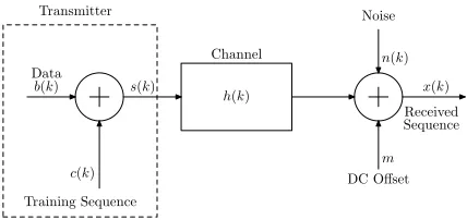
The familiar system set-up required for the ST method is depicted in Fig. 1 [1]. Accordingly, the received data block in the ST method has the following form [1, 2]:

x(k) =

M−1

X

l=0

h(l)b(k−l)+

M−1

X

l=0

h(l)c(k−l)+n(k)+m

c(k)

Training Sequence Data

b(k) s(k) Transmitter

h(k) Channel

DC Offset

m

Received Sequence

x(k)

n(k) Noise

Fig. 1. The mathematical model for ST.

response,n(k) is the noise andmrepresents an un-known DC-offset term due to using first-order statis-tics (see (2)) with non-ideal r.f. receivers (see [1]). Furthermore,c(k)is the superimposed training sequen-ce of mean ¯c = 1

NP

PP−1

k=0 c(k) and power σc2 = 1

NP

PP−1

k=0 |c(k)|2, periodic with periodP ≥M. We will assume the following:

H1) All terms in (1) can be complex valued.

H2) The sequences b(k)andn(k) are independent and identically distributed (i.i.d.) random sequen-ces of zero mean.

H3) The channel is of orderM −1—i.e. h(0)6= 0

andh(M−1)6= 0.

H4) The channel order is known.

Under H2 and the periodicity of the training se-quence, we can see from (1) that the output sequence x(k)is first-order cyclostationary of periodP. Thus, we can define its cyclostationary mean

y0(j) :=E[x(iP+j)] = M−1

X

l=0

h(l)c(j−l)P+m (2)

withj = 0, ... , P −1 where(·)P indicates arith-metic modulo-P, and the subscript ‘0’ indicates that it is a fixed (deterministic) value as opposed to a gen-eral variabley(j), and this nomenclature will be used throughout the rest of the paper. Equation (2) can be written in matrix form as

y₀=C[M]h0+m0 (3)

whereC[M]isP×Mandh0= [h(0), h(1), ..., h(M− 1)]T

isM×1;y₀= [y0(0), y0(1), ... , y0(P−1)]T andm0 = [m, ... , m]T are both P ×1. Matrix C[M] corresponds to the first M columns of matrix C=circ(c(0), c(P−1), c(P−2), ... , c(1)), where the operation ‘circ’ produces a circulant matrix [5]. MatrixCis thus composed ofC[M]in (3) and its ‘com-plement’ChP₋M_i, i.e. the lastP−M columns ofC, where

C≡C[M_]|C_hP₋M_i

. (4)

To make the subspace interpretation that follows meaningful, we requireC to be full rank. Note that

this is not a necessary condition for channel estima-tion using ST assuming perfect TSS, as was shown in [6]. To makeCfull rank, we are going to use op-timum channel independent (OCI) training sequences that were introduced in [1]. These also give,CHC=

CCH = P σ2

cIP_×P, simplifying the projection opera-tion between subspaces. Thus, from the least squares solution to (3), the filter coefficients are obtained by (noting thatCH_[M_]C[M] =P σc2IM×M)

h0= 1

P σ2 c

CH_[M](y0−m0). (5)

In the situation where there is no TSS, once the cyclic means in (2) are computed, there is no way to say which of them corresponds toj = 0,j = 1and so on. The only thing we know is that they appear se-quentially and that the computed cyclostationary mean is an unknown cyclic permutationP0y0of the true one (y₀), due to the periodicity ofc(k). It is important to note that a matrixP0 that performs a cyclic permu-tation operation on a vector is a circulant matrix as well. The vectorm0 is not affected by any (cyclic) permutation because all its components are equal and som0=P0m0.

ForP = M, and no TSS, the solution to (3) is a cyclically permuted version of the true channel co-efficient vector,P0h0. This solution is obtained from (5) withy₀ replaced byP0y0, makingm0 = P0m0, and noting thatCP0 =P0C—i.e. circulant matrices commute [5]. Thus, TSS reduces to finding the correct permutationP0, as was (implicitly) done in [1].

For P > M, the channel vector can not be re-trieved as in the previous paragraph (P = M), be-cause the matricesC[M_]andP0do not now commute. One possible option then is to pre-process the avail-able vectorP0y0and select the correcty0among a set of candidates, before solving (3).

Important clues to develop a new method for syn-chronisation can be derived from the previous para-graphs. Recall that the method in [1] (P = M) re-quired HOS and polynomial rooting, and so is rather complex. On the other hand, the method in [4] (P > M) uses the FFT and is simpler that the former. Fur-thermore, (5) obtains the channel vector just by pro-jecting on the subspace spanned by the columns of C[M](recall thatCis OCI). So we set out to investigate the advantages of using an overdetermined system of equations (P > M) and try to interpret the problem resolution as a projection process.

To start with, we study what happens to the cy-clostationary mean vector after a cyclic permutation. From the RHS of (3), we can confirm that after a cyclic permutation ofy₀,C_[M_]h0 will be the only affected term —recall thatm0is invariant under permutations. Thus, in the next Lemma we study the effect of a per-mutation onC[M]h0.

1vector. Then,PC[M]hcan be uniquely decomposed as

PC[M_]h=C_[M_](P[hT0TP₋M]

T )[M_]+

+ChP₋Mi(P[hT0TP₋M]

T )hP₋M_i

(6)

where0P−M is the column vector[0, ... , 0

| {z }

P−M

]T_{and for}

a vectorv,v[M_](v_hP₋M_i) are its firstM(lastP−M)

elements.

Proof: First note that C[M]h = C[hT 0TP−M]T ⇒ PC[M_]h = PC[hT 0TP₋M]T. Now, using the com-mutativity of circulant matrices, PC[hT 0TP−M]T = CP[hT0TP−M]T, and (6) follows from (4). The unique-ness comes becauseCis full rank. Q.E.D

The interpretation of Lemma 1 is clear. Consider the vector space spanned by the columns of matrixC, which are a base for this space as well becauseCis full rank. In turn,C[M]andChP−Mispan two subspaces

V andV⊥_{respectively, which are orthogonal because}

c(k)is OCI. Assume for the moment thatm= 0in (3). The true cyclostationary mean vectory₀ lies exactly onV—i.e. it is a linear combination of the columns of C_[M_]—but any cyclic permutationP6=Iof it will have components inV⊥ _{as well. This important property}

can be used to achieve TSS in the DC-offset free case. The next section proposes a general method to deal with TSS in the presence of a non-zero DC-offset.

3. Proposed training sequence

syn-chronisation method

Because of the lack of TSS, assume that the cyclic permutation of the cyclostationary mean available at the receiver isP0y0. To work with the most general case possible, a DC-offset will be taken into account as well. Let us now consider the decomposition ofP0y0 inV andV⊥_.

So, applying a cyclic permutation operator to both sides of (3), we need to know the decomposition of the permutedC[M]h and the decomposition of (the per-muted)m0. The former is given by Lemma 1 while the decomposition of the DC-offset term is given by

m0=C[M]m˜0[M]+ChP−Mim˜0hP−Mi (7)

wherem˜0is aP×1vector of constant elements m P_¯c, as can easily be confirmed. So from (3), and using (7) and Lemma 1, then we have,

P0y0=C[M](P0[hT00TP−M]

T₎

[M]+

+ChP−Mi(P0[hT00TP−M]

T_)h

P−Mi+

+C_[M_]m˜_0[M_]+C_hP₋M_im˜_0hP₋M_i. (8)

Consider now the projection ofP0y0onto theV⊥

space. So, multiply both sides of (8) byP σ12 c

CH_hP−Mi:

1

P σ2 c

CH_hP−MiP0y0=

=(P0[hT00

T

P₋M]T)hP−Mi+ ˜m0hP−Mi.

(9)

Now, two different cases are clearly distinguishable:

C1) ForP0=Ithe RHS of (9) reduces tom˜0hP₋M_i —i.e., a vector with all its components of equal value m

P¯c.

C2) ForP06=Ithe first term of the RHS of (9) does not vanish, and thus, we will not have a vector of equal components.

Note that C2 is only validin general. The conditions under which C2 isalwaystrue will be discussed shortly. The properties of (9) under cases C1 and C2 can be used for TSS, but prior to the formalisation of these properties in form of a useful proposition, it is neces-sary to develop a measure of how equal are the ele-ments of a vector. So, define the operatorJ {v} = kv−¯vk2_{, where¯v= [¯v, ... , ¯v]}T_{andv¯is the mean of}

all the elements ofv. The desired property ofJ {v}

is thatJ {v}= 0iff all the elements ofvare equal to each other (and thus, equal to the mean).

Proposition 1 LetP ≥2M + 1, hereafter known as

the strong constraint, thenJnCH_hP₋M_iP0y0

o

= 0iff P0=I.

Proof:The necessary condition (⇐) is proved by C1. For the sufficient condition (⇒), we need to find the conditions under which C2 is always true for allP0, y₀ and OCI c(k). Thus, let us work with the worst case scenario—i.e. when all theM components ofh0 are equal. So, if we require(P0[hT0 0P−M]T)hP−Mi

not to be a vector of equal components for anyP06=I andh06=0M, then we require that its length is larger thatM—i.e.P−M > M. Q.E.D

TSS is finally achieved as follows. The available cyclic permutation of the cyclostationary mean vector, P0y0, is cyclically permuted by all the cyclic permu-tations ofP elements. The cyclic permutationPP0y0 ofP0y0minimising the operatorJ

n

CH_hP−MiPP0y0

o

is the true cyclostationary mean vectory₀. This fol-lows because by proposition 1 PP0 = I, and thus PP0y0=y0.

Oncey₀ is known, the DC-offsetmcan be com-puted, using (9) under case C1, from any of the ele-ments ofCH_hP−Miy0. Nevertheless, we propose to per-form an average of the elements ofCH_hP−Miy0because when it comes to the practical implementation of the method, i.e. estimation, the average will of course give a smaller variance. So,

m= ¯c

σ2 c

1

P−M[1|, ... ,{z 1}

P₋M

andmis the mean just mentioned normalised by the quotient between the mean (¯c) and the power (σ2

c) of the training sequence.

Finally, oncey₀andmare known, the channel co-efficients can then be computed from (5).

3.1 Relaxing assumption H4 —conditions for equal-isation

The assumption H4 is required in order to apply Propo-sition 1, which is the basis of the TSS method pre-sented here. The channel order is needed twice in Proposition 1. Firstly, so that the strong constraint can be enforced; secondly, it appears in the argument of the operatorJ. If H4 is not fulfilled, the channel cannot be estimated. Nevertheless, when it comes to equalisation what is needed is just an upper bound for the channel order, as it will be shown next.

The effects of using an upper bound are then two-fold. Firstly, the range of values ofP satisfying the strong constraint is included in the range of values ob-tained if the actual channel order is used. So, no prob-lem is encountered here. Secondly, if the channel order is assumed to be bigger than what it actually is, then h0will have extra zero taps at the tails. This will allow the operatorJ to give more than one possible solution following proposition 1. Anyway, all the allow solu-tions obtained will be related by a linear shift and the only effect on equalisation is a delay. This delay can also appear in a practical implementation of the pro-posed TSS method, if the first or last of the channel taps is very close to zero.

4. Actual application of the method

In an actual application, the elements of the cyclosta-tionary mean vectory₀have to be estimated using, as usual, time averages:yˆ0(j) =N1P

PNP−1

i₌₀ x(iP+j), j= 0, 1, ... , P−1. But because of lack of TSS, this estimate will correspond to an unknown cyclic permu-tation ofy₀, i.e. P0ˆy0. To simplify notation, replace P0ˆy0 byˆy

(P0)

0 . Based on this estimate, the TSS, the DC-offset estimation and the channel estimation are sequentially obtained as shown in Table 1.

4.2 Computational burden

Consider the overall computational burden of the prac-tical implementation, in terms of total products and di-visions. For the proposed method in Table 1, the com-putational burden isP3_{+ (1−M)P}2_{+ 2P+ 3, i.e.}

O(P3_{); for the method in [4], the computational} bur-den isM N P + 2P3_{+ (M+ 1)P}2_{−(M+ 2)P+ 1,} i.e.O(M N P). The filtering steps required in [4], con-tributing toward theM N P term, can be a significant part of the computational burden of [4]. For exam-ple, letN =O(P3_{)andM =O(P)as in [4] and as} in the following simulation, thenO(M N P)becomes

O(P5_).

Cyclostationary mean estimation:

ˆ y(P0)

0 (j) = N1P

PNP−1

i=0 x(iP+j+k0)

j= 0,1, ... , P−1

wherek0is an unknown synchronisation offset.

Training sequence synchronisation:

{Pl} P

l=1=set of allP×Pcyclic permutation matrices. ComputePopt=arg min

Pl n

JnCHhP−MiPlˆy(

P0) 0

oo

DC-offset estimation:

ˆ

m= c¯

σ2 c

1

P−M[1, ... , 1

| {z }

P−M

]CH_hP₋M_iPoptˆy(

P0) 0

Channel estimation:

From (5),ˆh0 =P σ12 cC

H

[M] 

Poptˆy(0P0)−[ ˆm, ... , mˆ

| {z }

P

] 

.

Table 1. Proposed method for training sequence syn-chronisation of the ST method for channel estimation in the presence of DC-offset.

ComparingO(P3_{)of the proposed method with}

O(P5_{)of the method in [4], it is evident that the} com-putational burden reduction achieved with the new me-thod is very significant. And this reduction could be even bigger if the number of samplesN used in the estimation is increased.

5. Simulation

Three-tap Rayleigh fading channels were simulated. The channel coefficients were complex Gaussian, i.i.d. with unit variance. The average energy of the channel was set to unity. The data was a BPSK sequence, to which an OCI training sequence (see [1]) was added before transmission. The training to information power ratioTIR=σ

2 c σ2 b

ratio as defined in [2]

DCAC=m2_{/E|x(k)−n(k)−m|}2_.

In these simulations this was set to DCAC= 0.1. At each realisation, a random synchronisation offset be-tween 0 andN+P−1was introduced between trans-mitter and receiver, so we could be atanysample in-dex within the firstblock. After channel estimation, an MMSE equaliser, based on the channel estimates, of length 11 and optimum delay was used to compute the BER; 1000 realisations were averaged. As already mentioned at the end of subsection , we may have an unknown delay of the estimated channel with respect to the true one. In this particular case, it may hap-pen because of the randomness of the channel taps, so the first and last channel tap could be close to, or even, zero. Thisidentification delay, which in prac-tice has no major consequences, can worsen the sim-ulated BER, misleading the performance analysis of the method. To avoid this, the identification delay was computed by comparing the equalised symbols with the true ones, for different delays, and choosing the delay giving the smallest BER—this problem was re-ported in [4] as well. For a comparison between the TSS methods in [1] and [4], please refer to [4], where simulations show that the later clearly outperforms the former.

0 5 10 15 20 25

10−2 10−1 100

SNR (dB)

Channel estimates MSE (dB)

1: Method in [4]. 2: ST/Table I.

3: ST, exact synchronization and DC−offset known.

Fig. 2. MSE of channel estimates, as a function of

the SNR, computed following Table 1. The identifica-tion delay has been considered. The estimates assum-ing known DC-offset and perfect TSS are included, to-gether with the TSS method in [4], for comparison pur-poses. Note that methods 1 and 2 are indistinguishable on the graph.

Figure 2 shows the MSE of the channel estimate obtained with the method presented in Table 1. The MSE obtained with the ST method assuming perfect TSS is plotted as well as a benchmark. The proposed method (with no TSS) is not very much different. Fi-nally, compared with the method in [4], the best pub-lished TSS method for ST so far, we can see that our

0 5 10 15 20 25

10−3 10−2 10−1 100

SNR (dB)

BER

1: Method in [4]. 2: ST/Table I.

3: ST, exact synchronization and DC−offset known.

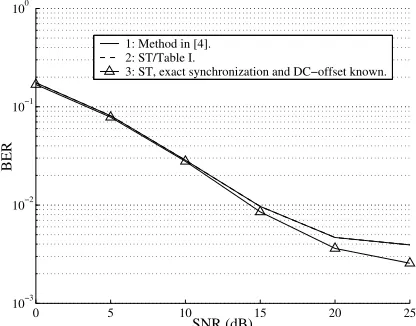
Fig. 3. BER versus SNR obtained using the algorithm of Table 1. Note that methods 1 and 2 are indistin-guishable on the graph.

proposed method gives identical results, but with the already mentioned, huge reduction in computational burden.

Figure 3 shows the BER of the proposed method and that of the ST with perfect TSS. The method in [4] is included as well for comparison. The conclusions drawn in the previous paragraph are equally applicable here too.

6. Conclusions

7. REFERENCES

[1] A. G. Orozco-Lugo, M. M. Lara, and D. C. McLernon, “Channel estimation using implicit training,” IEEE Trans. Signal Processing, vol. 52, pp. 240–254, 2004.

[2] J. K. Tugnait and W. Luo, “On channel estimation using superimposed training and first-order statis-tics,” IEEE Commun. Lett., vol. 7, pp. 413–415, 2003.

[3] M. Ghogho, D. C. McLernon, E. Alameda-Hernandez, and A. Swami, “Channel estimation and symbol detection for block transmission us-ing data-dependent superimposed trainus-ing,”IEEE Signal Processing Lett., vol. 12, pp. 226–229, 2005.

[4] J. K. Tugnait and X. Meng, “Synchroniza-tion of superimposed training for channel esti-mation,” Proceedings of International Confer-ence on Acoustics, Speech and Signal Processing ICASSP04, vol. IV, pp. 853–856, 2004.

[5] P. J. Davis, Circulant Matrices, Chelsea Publish-ing, New York, N.Y., 1994.

[6] M. Ghogho and A. Swami, “Improved chan-nel estimation using superimposed training,” in