SimCrime: A Spatial Microsimulation Model for the Analysing of Crime in Leeds.

White Rose Research Online URL for this paper:

http://eprints.whiterose.ac.uk/4982/

Monograph:

Kongmuang, C., Clarke, G.P., Evans, A.J. et al. (1 more author) (2006) SimCrime: A

Spatial Microsimulation Model for the Analysing of Crime in Leeds. Working Paper. The

School of Geography, University of Leeds

School of Geography Working Paper 06/1

[email protected] https://eprints.whiterose.ac.uk/

Reuse

Unless indicated otherwise, fulltext items are protected by copyright with all rights reserved. The copyright exception in section 29 of the Copyright, Designs and Patents Act 1988 allows the making of a single copy solely for the purpose of non-commercial research or private study within the limits of fair dealing. The publisher or other rights-holder may allow further reproduction and re-use of this version - refer to the White Rose Research Online record for this item. Where records identify the publisher as the copyright holder, users can verify any specific terms of use on the publisher’s website.

Takedown

If you consider content in White Rose Research Online to be in breach of UK law, please notify us by

SimCrime: A Spatial Microsimulation Model

for the Analysing of Crime in Leeds

Charatdao Kongmuang, Graham P Clarke,

Andrew J Evans and Jianhui Jin

Version 1.1

December 2006

All rights reserved

School of Geography, University of Leeds

Leeds, LS2 9JT, United Kingdom

This Working Paper is an online publication and may be revised. Our full contact details are:

Mail address:

School of Geography University of Leeds Leeds, LS2 9JT United Kingdom

Fax: +44 (0) 113 343 3308

Email:

Charatdao Kongmuang

[email protected]

Prof. Graham P Clarke

[email protected]

Dr. Andrew J Evans

[email protected]

Jianhui Jin

Acknowledgements

a. The 2001 Census statistics used in this thesis are Crown Copyright and are produced by the Office for National Statistics (ONS). The statistics are licensed for academic use by the ESRC/JISC Census Programme, which funded access to the data for researchers in UK, free at the point of use. The ESRC/JISC Census Programme funds the Data Support Units which provide access to UK Census Data. The 2001 Census Area Statistics are provided by the Census Dissemination Unit (CDU) through the Manchester Information and Associated Services (MIMAS) of Manchester Computing, University of Manchester through an interface called CASWEB.

b. All maps are based on data provided by the United Kingdom Boundary Outline and

Reference Database for Education and Research Study (UKBORDERS) via Edinburgh University Data Library (EDINA) with the support of the Economic and Social Research Council (ESRC) and the Joint Information Systems Committee (JISC) and boundary material which is copyright of the Crown, Post Office and the EDLINE consortium.

c. The 2001/2002 British Crime Survey, material from Crown copyright records made

available through the Home Office and the UK Data Archive has been used by permission of the Controller of Her Majesty’s Stationery Office and the Queen’s Printer for Scotland.

Abstract

Table of Contents

Acknowledgements ... iii

Abstract ... iv

Table of Contents ... v

List of Figures ... vi

List of Tables... vi

1. Introduction ... 1

2. Data Sources and Issues ... 2

2.1 The 2001 Census... 2

2.2 The 2001/2002 British Crime Survey ... 7

3. The Creation of Synthesis Microdata... 13

3.1 Synthetic Reconstruction ... 13

3.2 Combinatorial Optimisation... 14

4. Combinatorial Optimisation using Simulated Annealing Method ... 17

5. SimCrime Model Specification ... 20

5.1 Input ... 21

5.2 Input Adjustment ... 25

5.3 Model Execution Process... 27

5.4 Model Output... 32

6. Evaluation of Synthetic Microdata... 35

7. Concluding Comments... 40

References ... 41

List of Figures

Figure 1: Discrepancies in census counts between tables ... 7

Figure 2: Microsimulation procedure for the allocation of employment status ... 14

Figure 3: A simplified combinatorial optimisation process... 16

Figure 4: Flowchart of simulated annealing algorithm (after Pham and Karaboga, 2000)... 19

Figure 5: Constraint table adjusted method... 26

Figure 6: The process to check each individual fits the column constraints ... 29

Figure 7: SimCrime Framework ... 31

Figure 8: Distribution of females single, widowed, or divorced aged 25-49 living... 33

in rented house by output area in Leeds ... 33

Figure 9: Distribution of full-time students aged 20-30 living in rented ... 33

house by output area... 33

Figure 10: Distribution of high-class households with owner occupier... 34

having at least 1 car... 34

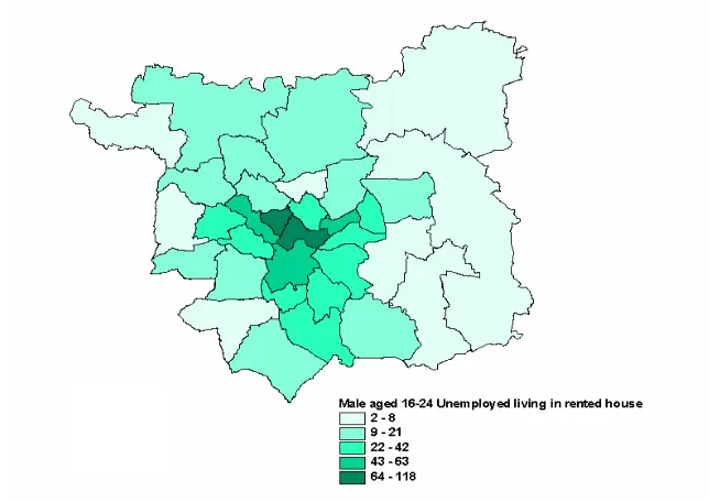
Figure 11: Distribution of males aged 16-24 unemployed and living in the... 34

rented house by ward ... 34

Figure 12: Spatial distribution of SAE for age and sex by living arrangement ... 39

at output area level. ... 39

Figure 13: Spatial distribution of SAE for NS-SEC by tenure type at ... 39

output area level. ... 39

Figure 14: Spatial distribution of SAE for tenure type and car or van... 40

availability by economic activity at output area level. ... 40

Figure 15: Spatial distribution of SAE for all constraints at output area level... 40

List of Tables

Table 2: Census Area Statistics dataset tables available from CASWEB... 5

Table 3: Selected topics in the British Crime Survey ... 8

Table 4: Comparing the British Crime Survey and police recorded crime ... 12

Table 5: Synthetic reconstruction versus combinatorial optimisation ... 17

Table 6: SimCrime constraint variables ... 23

Table 7: SimCrime constraint tables ... 24

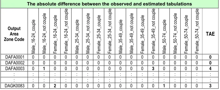
Table 8: Comparing the distribution of constraint table and synthetic microdata to get the Total Absolute Error (TAE). ... 36

8a: Constrainted table... 36

8b: The distribution of synthetic population ... 36

8c: Compare constraint table and the synthetic microdata to get TAE of each area ... 36

1.

Introduction

‘Microsimulation’ is a methodology aimed at building large-area datasets of individual units such as persons, households or firms (Clarke, 1996; Ballas and Clarke, 2000) and can be used to simulate the effect of changes in policy or other changes on these microunits. It essentially creates individual-level data from example individuals and aggregate statistics, matching the two together and allowing the merging of additional datasets. The microsimulation approach dates back to the work of Orcutt (1957) and Orcutt et al. (1961). It has been increasingly adopted to study the impacts of social and economic policies on individual units (Merz, 1991; Ballas et al., 2005), mainly for predicting the future effects of changing public policies (Clarke, 1996; Ballas and Clarke, 2001a, b). Spatial microsimulation combines the advantages of aspatial micro-analytical approaches with those of geographical models that take space into account. The key advantage of the spatial microsimulation approach is that it contains geographical information that can be used to investigate the local area impacts of policy changes. Spatial microsimulation is useful for modelling the socio-economic and spatial effects of policy changes at different geographical scales. Due to the advantages that it offers over traditional approaches, spatial microsimulation has become increasingly popular and a powerful tool within applications that have a geographical aspect.

SimCrime is a spatial microsimulation model that is designed to estimate the likelihood of being a victim of crime and crime rates at the small area level in Leeds and to answer what-if questions about the effects of changes in the demographic and socio-economic characteristics of the future population. The model is based on individual microdata. Specifically, SimCrime combines individual microdata from the British Crime Survey (BCS) for which location data is only at the scale of large areas, with census statistics for smaller areas to create synthetic microdata estimates for output areas (OAs) in Leeds using a simulated annealing method. The new microdata dataset includes all the attributes from the original datasets. This allows variables such as crime victimisation from the BCS to be directly estimated for OAs.

tables. The synthetic microdata is then evaluated in section 6. The final section gives some concluding comments.

2.

Data Sources and Issues

2.1 The 2001 Census

The census is a survey of the whole UK population. It has been carried out every ten years since 1801. The latest census was held on 29th April, 2001. The data in the census describes the characteristics of the population of the UK including demography, households, families, housing, ethnicity, birthplace, migration, illness, economic status, occupation, industry, workplace, transport mode to work, cars, and language (Rees et al., 2002). The questions listed in Table 1 allow the generation of results in a cross-tabulation format which is available for academic use. It provides a comprehensive spatial coverage. However, the output is modified when some numbers are involved and raw microdata itself is not released because of respondent confidentiality (Rees et al., 2002). Data are thus released for small areas only, e.g. output areas (OAs) or wards, and are not available at the individual or household level. The aggregate outputs are counts of people or households broken down by demographic and socio-economic characteristics. These are contained in a series of tables on a specific topic or area of interest. The 2001 Census aggregate statistics datasets include:

̇ Key Statistics: The Key Statistics datasets provide an overview and summary of the

main topics which are the most important and generally used statistics in a series of straightforward tables. It is available for all 2001 Census geographies.

̇ Standard Tables: The Standard Tables datasets provide the most detailed information

in a large number of cross-tabulated tables. It is available down to ward level in England, Wales and Northern Ireland, and postcode sector level in Scotland. It is not available for output areas.

̇ Standard Table Theme Tables: The Standard Tables Theme Tables are designed to

contain information about ranges of subjects related to particular themes available down to ward level in England, Wales and Northern Ireland, and postcode sector level in Scotland. It is not available for output areas.

̇ Census Area Statistics: Census Area Statistics provide the most detailed results

possible for smaller areas. They are generally produced for the same areas as the Key Statistics.

̇ Census Area Statistics Theme Tables: The Census Area Statistics dataset includes a

related to particular themes. They are available for the full range of 2001 Census geographies down to output areas.

̇ Census Area Univariate Tables: Available for the full range of 2001 Census

geographies down to output areas describing a single variable only.

̇ Armed Forces Tables: Provide information on members of the Armed Forces

available down to Local Authority District level for England and Wales only.

All of these datasets are available via Census Area Statistics Website (CASWEB).

The main dataset used in this study is the Census Area Statistics (CAS), which is equivalent to the Small Area Statistics (SAS) of the 1971, 1981, and 1991 Censuses. It is available for geographical levels down to output area (OA), the smallest unit of the 2001 Census geography. Each output area contains approximately 290 persons or 125 households. This is different from the 1991 Census when the smallest areas were Enumeration Districts (EDs) and electoral wards with an average size of about 180 and 2,000 households respectively (Dale and Teague, 2002). As mentioned above, the Census Area Statistics provide the most detailed results possible for smaller areas. In terms of data volume, it is the largest of the 2001 Census datasets, containing approximately 2 billion individual items of data. Table 2 shows the Census Area Statistics dataset tables available via Census Area Statistics Website (CASWEB), the academic web interface to census aggregate outputs and digital boundary data. Census Area Statistics dataset tables vary in size. The number of cells in a table range from 21 to 540 depending upon the number of variables involved and the number of categories. Larger tables provide more detailed information. However, the larger the tables are the greater the possible effect of data blurring as the likelihood of private data disclosure is greater as detail increases.

“The 2001 CAS will differ from the 1991 SAS in a significant respect. To avoid even the

perception of disclosure, counts in tables will not only be subject to imputation and record

swapping, but will also be randomly perturbed and rounded to the nearest three”

(Denham and Rees, 2002: 305)

Table 1: Topics in the 2001 Census

_____________________________________________________________________

No Topics

_____________________________________________________________________

For all properties occupied by households and all unoccupied Household accommodation:

1 The address, including postcode 2 Type of accommodation 3 Names of all residents

Names and usual addresses of visitors on census night (optional) 4 Tenure of accommodation

5 Whether rented accommodation is furnished or unfurnished (in Scotland only) 6 Type of landlord (for households in rented accommodation)a

7 Number of room

8 Availability of bath and toilet 9 Self-containment of accommodation

10 Lowest floor level of accommodation

11 Number of floor levels in the accommodation (in Northern Ireland only)

12 Availability of central heating

13 Number of cars and vans owned and available

For residents:

14 Name, sex, and, date of birth 15 Marital status

16 Relationship to others in household 17 Student status

18 Whether or not students live at enumerated address during term-time 19 Usual address one year ago

20 Country of birth

21 Knowledge of Gaelic (Scotland only), Welsh (Wales only), and Irish (Northern Ireland only)a 22 Ethnic groupa

23 Religion

24 Religion of upbringing (Scotland and Northern Ireland)

25 General health

26 Long-term illness

27 Provision of unpaid personal care

28 Educational and vocational qualifications 29 Economic activity in the week before the census

30 Time since last employment

31 Employment status

32 Supervisor status

33 Job title and description of occupation 34 Professional qualifications (England)

35 Size of workforce of employing organization at place of work

36 Nature of employer’s business at place of work (industry) 37 Hours usually worked weekly in main job

38 Name of employer 39 Address of place of worka 40 Means of travel to worka

41 Address of place of study (in Scotland only)

42 Means of travel to place of study (in Scotland only)

_________________________________________________________________

Source: Denham and Rees (2002), pp 311-312

Note: Bold indicates a new question (compared with the 1991 Census);

Italic indicates a question to be used in only one part of the United Kingdom.

Table 2: Census Area Statistics dataset tables available from CASWEB

Census Area Statistics dataset tables

CS001 Age by Sex and Resident Type: All People CS002 Age by Sex and Marital Status: All People

CS003 _{Age of Household Reference Person (HRP) by Sex and Marital Status (Headship):} All Households

CS004 Age by Sex and Living Arrangements: All People in Households

CS011 Family Composition by Age of Family Reference Person (FRP): All Families

CS012 Schoolchildren and Students in Full-Time Education Living Away from Home in Term-Time by Age: All Schoolchildren and Students in Full-Time Education who Would Reside in the Area were they not Living Away from Home During Term-Time

CS013 Age of Household Reference Person (HRP) and Tenure by Economic Activity of HRP: All Households with HRP Aged 16 to 74

CS016 Sex and Age by General Health and Limiting Long-Term Illness (LLTI): All People in Households

CS017 Tenure and Age by General Health and Limiting Long-Term Illness (LLTI): All People in Households

CS019 General Health, Limiting Long-Term Illness (LLTI) and Occupancy Rating by Age: All People in Households

CS020 Limiting Long-Term Illness (LLTI) and Age by Accommodation Type and Lowest Floor Level of Accommodation: All People in Households

CS021 Economic Activity by Sex and Limiting Long-Term Illness (LLTI): All People Aged 16 to 74

CS023 Age and General Health by NS-SeC: All People Aged 16 to 74

CS025 Sex and Age by General Health and Provision of Unpaid Care: All People in Households

CS026 Sex and Economic Activity by General Health and Provision of Unpaid Care: All People Aged 16 to 74 in Households

CS027 Households with a Person with a Limiting Long-Term Illness (LLTI) and their Age by Number of Carers in Household and Economic Activity: All Households

CS029 Sex and Age by Hours Worked:

All People Aged 16 to 74 in Employment the Week Before the Census

CS030 Sex and Economic Activity by Living Arrangements: All People Aged 16 to 74 in Households

CS032 Sex, Age and Level of Qualifications by Economic Activity: All People Aged 16 to 74

CS033 Sex and Occupation by Age:

All People Aged 16 to 74 in Employment the Week Before the Census

CS034 Former Occupation by Age:

All People Aged 16 to 64 not in Employment the Week Before the Census

CS035 Sex and Occupation by Employment Status and Hours Worked: All People Aged 16 to 74 in Employment the Week Before the Census

CS038 Sex and Industry by Employment Status and Hours Worked:

All People Aged 16 to 74 in Employment the Week Before the Census

CS039 Occupation by Industry:

CS040 Sex and Occupation by Hours Worked:

All People Aged 16 to 74 in Employment the Week Before the Census

CS041 Economic Activity and Time Since Last Worked by Age: All People Aged 16 to 74 CS042 NS-SeC by Age: All People Aged 16 to 74

CS043 Sex and NS-SeC by Economic Activity: All People Aged 16 to 74

CS044 NS-SeC of Household Reference Person (HRP) by Household Composition: All HRPs Aged 16 to 74

CS045 NS-SeC of Household Reference Person (HRP) by Age (of HRP): All HRPs Aged 16 to 74

CS046 NS-SeC of Household Reference Person (HRP) by Tenure: All HRPs Aged 16 to 74 CS047 NS-Sec by Tenure: All People in Households Aged 16 to 74

CS048 Dwelling Type and Accommodation Type by Household Space Type: All Household Spaces. All Dwellings

CS049 Dwelling Type and Accommodation Type by Tenure (Households and Dwellings): All Occupied Household Spaces. All Occupied Dwellings

CS050 Dwelling Type and Accommodation Type by Tenure (People): All People in Households

CS051 Tenure and Household Size by Number of Rooms: All Households CS052 Tenure and Persons Per Room by Accommodation Type: All Households CS053 Household Composition by Tenure and Occupancy Rating: All Households CS055 Dwelling Type, Accommodation Type and Central Heating by Tenure:

All Households

CS056 Tenure and Amenities by Household Composition: All Households

CS059 Accommodation Type and Car or Van Availability by Number of People Aged 17 Or Over in the Household: All Households

CS060 Tenure and Car or Van Availability by Number of People Aged 17 Or Over in the Household: All Households

CS061 Tenure and Car or Van Availability by Economic Activity: All People Aged 16 to 74 in Households

CS066 Sex and Approximated Social Grade by Age: All People Aged 16 and Over in Households

CS067 Age of Household Reference Person (HRP) and Dependent Children by Approximated Social Grade: All Households

CS068 Age and Dependent Children by Household Type (Household Reference Persons): All HRPs

CS103 Sex and Age by Religion: All People

CS105 Age by Highest Level of Qualification: All People Aged 16 to 74 CS113 Occupation by Highest Level of Qualification: All People Aged 16 to 74 CS114 NS-SeC by Highest Level of Qualification: All People Aged 16 to 74

CS118 Number of Employed People and Method of Travel to Work by Number of Cars or Vans in Households: All Households with at Least One Person Working in the Week Before the Census

CS119 Sex and Age by Method of Travel to Work:

All People Aged 16 to 74 Working in the Week Before the Census CS122 NS-SeC by Method of Travel to Work:

All People Aged 16 to 74 Working in the Week Before the Census

Source: 2001 Census Area Statistics

Note: Release of Census Area Statistics tables 15, 62, 64, 65 and 133 has been postponed pending the

Figure 1: Discrepancies in census counts between tables

Source: 2001 Census Area Statistics

Note: Each cell shows the number of people aged 16-74 living in households

2.2 The 2001/2002 British Crime Survey

The British Crime Survey (BCS) produced by the Home Office is one of the largest social research surveys conducted in England and Wales. The BCS was first carried out in 1982 and further surveys were carried out in 1984, 1988, 1992, 1994, 1996, 1998, 2000 and 2001 respectively. The surveys have been carried out on a continuous basis since April 2001 and results from that point have been reported by financial year. The BCS is primarily a victimisation survey and is a very important source of information about levels of crime and public attitudes to crime. People do not always report crimes to the police for a variety of reasons and those crimes are therefore excluded in police recorded crime statistics. In the BCS the respondents are asked about their experiences of property crimes of the household (e.g.

ethnicity, economic activity, socio-economic group, household income, car ownership, number of adults/children in households, long-term illness) and area characteristics, all of which play an important role in this study.

The 2001/2002 BCS had a target sample of 40,000 households in England and Wales. The respondents were randomly selected from the Post Office’s list of addresses in England and Wales. Therefore it has a good mix of people from different ages, backgrounds and situations. The 2001/2002 BCS represented two linked populations: households in England and Wales living in private residential accommodation, and adults aged 16 and over living in such households. It has been noted that the BCS does not count all crimes that occur in England and Wales, but it does provide a consistent measure of trends in crime from one year to the next. Moreover, the BCS gives a more accurate picture of crime levels and trends compared with the police recorded crime, because it asks people about their actual experiences (thus covering crimes that do not get reported to the police).

However, there are some limitations with the BCS. Firstly, the BCS only surveys people aged 16 and over in private households. Therefore it does not include crime against people aged under 16 and it does not cover the population resident in student Halls of Residence, those in residential care, those in prison, or members of the armed forces. Secondly, it does not cover certain types of crime including: victimless crime (drug offences), fraud, sexual offences and homicide because the victims cannot be interviewed (while police recorded crime does) (Table 4). Thirdly, while the BCS provides a picture of crime at the national level, it cannot tell us what is happening in the local authority or neighbourhood as the police recorded data can. Thus, the BCS cannot identify small area hotspots or high risk areas.

Table 3: Selected topics in the British Crime Survey

_______________________________________________________________________

Selected topics in the British Crime Survey

Area Characteristics:

Inner city flag

Area type: Inner-city/Urban/Rural Standard Region

Government Office Region ACORN type:

ACORN Group ACORN category ACORN change type ACORN change group Police Force Area

ONS Ward Classification : Group

Council areas (based on ACORN type) Government Office Region (Grouped) Area type: Rural/Not rural

Neighbourhood type Structure of household

Respondent:

Sex Age

Marital status

ONS harmonised marital status Whether respondent living in a couple Cohabiting status

HRP status/Respondent status Ethnic status

Respondent Socio-Economic Classification (NS-SEC) - Operational Categories Respondent Socio-Economic Classification (NS-SEC) - Analytic Categories Respondent Socio-Economic Group (SEG)

Respondent employment status

Are you a full-time student at college or university Respondent on government training scheme Respondent away from job

Whether respondent full-time student Respondent working full-time or part-time

Respondent working as employee or self-employed Respondent managerial status

Whether respondent employs people or not Highest qualification

Cultural background

In which way do you occupy this accommodation Who is your landlord

ONS Harmonised Tenure type ONS harmonised accommodation type Number of adults in household

Number of children under 16 in household Number of cars

Total household income in last year Personal earnings of respondent in last year Personal earnings of partner in last year Total household income (4 bands) Total household income (5 bands) Total household income (6 bands) Is respondent victim or not

ONS harmonised long-standing illness

Respondent Lifestyle:

No. visits pub/wine bar evening last month

How often have you visited a nightclub in last month How often do you drink alcohol

How many units of alcohol do you drink

How many hours spent away from home during day Household occupied during day

Number of hours home left unoccupied on average Is home ever left unoccupied during weekdays

Household Reference Person:

Age of Household Reference Person Sex of Household Reference Person

Marital status

Cohabiting status HRP social class Ethnic Group Disability/illness Number of cars

HRP Socio-Economic Classification (NS-SEC) - Operational Categories HRP Socio-Economic Classification (NS-SEC) - Analytic Categories HRP Socio-Economic Group (SEG)

Household reference person employment status

HRP: On a government scheme for employment training Is HRP a full-time student at college or university Whether Household Reference Person full-time student Household Reference Person on government training scheme Household Reference Person away from job

Household Reference Person working full-time or part-time

Household Reference Person working as employee or self-employed Household Reference Person managerial status

Whether HRP employs people or not

Victim Experiences:

If vehicle stolen or driven away without permission How many times has this happened (MotTheft)) If something stolen off or out of vehicle How many times has this happened (MotStole) If vehicle tampered with or damaged

How many times has this happened (CarDamag) Owned a bicycle at any time in reference period How many bicycles does household own If bicycle stolen

How many times has this happened (BikTheft)

If anyone got into previous residence to steal/try to steal How many times has this happened (PrevThef)

If anyone got into previous residence and caused damage How many times has this happened (PrevDam)

If anyone tried to get into previous residence to steal/cause damage How many times has this happened (PrevTry)

If anything was stolen out of previous residence How many times has this happened (PrevStol)

If anything was stolen from outside previous residence How many times has this happened (PrOside)

If anything was damaged outside previous residence How many times has this happened (PrDeface)

If anyone got into current residence to steal/try to steal (Movers) How many times has this happened (HomeThef)

If anyone got into current residence to steal/try to steal (Non-movers) How many times has this happened (YrHoThef)

If anyone got into current residence and caused damage How many times has this happened (YrHoDam)

If anyone tried to get into current residence to steal/cause damage How many times has this happened (YrHoTry)

If anything was stolen out of hands pockets or bag How many times has this happened (PersThef)

If anyone tried to steal anything from hands pockets or bag How many times has this happened (TryPers)

If anything has been stolen from a cloakroom office etc How many times has this happened (OtheThef) If personal items have been deliberately damaged How many times has this happened (Delibdam)

If anyone has deliberately used force/violence on respondent How many times has this happened (Delibvio)

If anyone has threatened to damage things/use force or violence How many times has this happened (ThreViol)

If respondent has been sexually assaulted or attacked How many times has this happened (SexAttak)

If member of household has used force or violence on respondent How many times has this happened (HhldViol)

Have you ever been victim of crime reported to police Have you been the victim of crime in last 2 years Have you ever been arrested by police

Have you been arrested by police in last 2 years Have you ever been in court during a criminal case Have you been in court in last 2 years

Have you ever been a juror in criminal case

Have you been a juror in a criminal case in last 2 years Have you ever been in court as the accused

Have you been in court as the accused in last 2 years Have you ever been in contact with probation service

Have you been in contact with probation service in last 2 years Have you ever been inside a prison

Have you been inside a prison in last 2 years

Have you been the victim of a vehicle crime in last 5 years How many times have you been the victim of vehicle crime Have you been insulted pestered or intimidated

How many times have you been insulted or intimidated How many people insulted or intimidated you

How well did you know person insulting you Any fires in last 12 months

How many fires in the last 12 months Was the Fire Brigade called

____________________________________________________________________

Source: The 2001/2002 British Crime Survey, Crown Copyright.

Note: A Classification of Residential Neighbourhoods (ACORN) variables are not included in

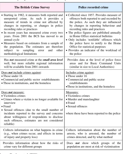
Table 4: Comparing the British Crime Survey and police recorded crime

The British Crime Survey Police recorded crime

̇ Starting in 1982, it measures both reported and unreported crime. As such it provides a measure of trends in crime not affected by changes in reporting, or changes in police recording rules or practices

̇ In recent years has measured crime every two years. From 2001 the BCS has moved to an annual cycle

̇ Measures based on estimates from a sample of the population. The estimates are therefore subject to sampling error and other methodological limitations

̇ Collected since 1857. Provides measure of offences both reported to and recorded by the police. As such they are influenced by changes in reporting behaviour and recording rules and practices

̇ The police figures are published annually in Home Office statistical bulletins ̇ Only includes ‘notifable’ offences which

the police have to notify to the Home Office for statistical purposes

̇ Provides an indicator of the workload of the police

Has not measured crime at the small area level well, but more reliable regional information will be available from 2001 onwards

Provides data at the level of police force areas and for Basic Command Units (similar in size to Local Authorities)

Does not include crimes against: ̇Those under 16

̇Commercial and public sector establishments ̇Those in institutions, and the homeless

Includes crime against: ̇Those under 16

̇Commercial and public sector establishments

̇Those in institutions, and the homeless

Does not measure: ̇ Victimless crimes

̇ Crimes where a victim is no longer available for interview

̇ Fraud

̇ Sexual offences (due to the small number of incidents reported to the survey and concerns about willingness of respondents to disclose such offences, estimates are not considered reliable)

Measures:

̇Victimless crimes ̇Murder and manslaughter ̇Fraud

̇Sexual offences

where these have been reported to the police

Collects information on what happens in crime

(e.g., when crimes occur, and effects in terms of injury and property loss)

Collects information about the number of arrests, who is arrested, the number of crimes detected, and by what method

Provides information about how the risks of crime vary for different groups

Does not show which groups of the population are most at risk of victimisation

3.

The Creation of Synthesis Microdata

Although many countries, for example Sweden, have a microdata database, because of confidentiality problems, in the UK we do not have a microdata database on individuals and households. Thus, it is useful to create synthetic microdata. Synthetic reconstruction and combinatorial optimisation are the two main approaches used to create small area population microdata which comprise lists of individuals along with an associated set of individual characteristics. (Williamson et al., 1998; Williamson, 2002).

3.1 Synthetic Reconstruction

Figure 2: Microsimulation procedure for the allocation of employment status

(after Clarke, 1996)

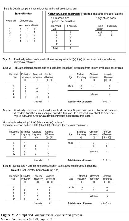
3.2 Combinatorial Optimisation

An alternative approach to generate synthetic microdata dataset is the combinatorial

optimisation approach (Figure 3). The process involves selecting the combination of household records from available microdata which offers the best fit for known constraints in the selected small area. Williamson et al. (1998) describe this process in more detail and explore various techniques of combinatorial optimisation including the hill climbing approach, the generic algorithm approach, and the simulated annealing approach. They found that modified simulated annealing stands out as the best solution. They estimated small area populations by combining information contained in the Sample of Anonymised Records (SAR) and the census Small Area Statistics (SAS) tables from the 1991 Census. The process starts from an initial set of households chosen randomly from the SAR. These are randomly allocated into SAS areas until the number of households matches the number reported by the SAS tables. The other SAS aggregate statistics are then generated (for example the gender distribution). One household is

Household head (hh)

Steps 1st 2nd Last

1. Age, sex, and marital status (M) of household head (From SAS Table 39)

2. Probability of employment status of household head, given age, sex, and marital status (From SAS Table 34)

3. Random number (Computer generated)

4. Employment status assigned on the basis of random sampling

5. Next household head (repeat until all household heads assigned an employment status)

Age: 19 Sex: Male M: Married

Age: 25 Sex: Male M: Married

Age: 65 Sex: Female M: SWD

0.6 0.6 0.0

0.43 0.38 0.27

then randomly replaced with a new household from the SAR, and the aggregate statistics reassessed. If the replacement improves the fit, the households are swapped. Otherwise, the swap is made or not made on the basis of the simulated annealing algorithm. The process is repeated with the aim of gradually improving the fit between the observed data and the selected combination of SAR households. Given computational time limits, the final combination is the best achievable rather than the guaranteed optimal solution (Huang and Williamson, 2001).

Synthetic reconstruction and combinatorial optimisation methodologies for the creation of small area synthetic microdata have been examined by Huang and Williamson (2001). They found that outputs from both methods can produce synthetic microdata that fit constraining tables very well. However, the dispersion of the synthetic data has shown that the variability of datasets generated by combinatorial optimisation is much less than by synthetic reconstruction, at ED and ward levels. The main problem for the synthetic reconstruction is that a Monte Carlo solution is subject to sampling error which is likely to be more significant where the sample sizes are small. Ordering is also important in the generation of new characteristics (Clarke,

1996). The ordering of conditional probabilities can also be a problem as synthetic

reconstruction is a sequential procedure. The degree of error will increase when we go further

along the chain in the generation of characteristics. Another drawback of synthetic

Step 1: Obtain sample survey microdata and small area constraints

Step 2: Randomly select two household from survey sample [ (a) & (e) ] to act as an initial small area microdata estimate

Step 3: Tabulate selected households and calculate (absolute) difference from known small area constraints

Household Estimated Observed Absolute Estimated Observed Absolute

Size frequency frequency difference Age frequency frequency difference

(i) (ii) (i) – (ii) (i) (ii) (i) – (ii)

1 0 1 1 adults 4 3 1

2 1 0 1 1 2 1

3 1 0 1

4 0 1 1 Sub-total: 2

5+ 0 0 0

Sub-total: 4 Total absolute difference = 4 + 2 = 6

Step 4: Randomly select one of selected households (a or e). Replace with another household selected at random from the survey sample, provided this leads to a reduced total absolute difference. **(The simulated annealing algorithm introduce additional at this stage)**

Households selected: (d) & (e) [Household (a) replaced]

Tabulate selection and calculate (absolute) difference from known constraints

Household Estimated Observed Absolute Estimated Observed Absolute

size frequency frequency difference Age frequency frequency difference

(i) (ii) (i) – (ii) (i) (ii) (i) – (ii)

1 1 1 0 adults 3 3 0

2 0 0 0 1 2 1

3 1 0 1

4 0 1 1 Sub-total: 1

5+ 0 0 0

Sub-total 2 Total absolute difference = 2 + 1 = 3

Step 5: Repeat step 4 until no further reduction in total absolute difference is possible:

Result: Final selected households: (c) & (d)

Household Estimated Observed Absolute Estimated Observed Absolute

size frequency frequency difference Age frequency frequency difference

(i) (ii) (i) – (ii) (i) (ii) (i) – (ii)

1 1 1 0 adults 3 3 0

2 0 0 0 2 2 0

3 0 0 0

4 1 1 0 Sub-total: 0

5+ 0 0 0

Sub-total 0 Total absolute difference = 0 + 0 = 0

Figure 3: A simplified combinatorial optimisation process Source: Williamson (2002), page 237

Survey Microdata

Household Characteristics

size adults children

(a) 2 2 0

(b) 2 1 1 (c) 4 2 2 (d) 1 1 0 (e) 3 2 1

Known small area constraints [Published small area census tabulations]

1. Household size 2. Age of occupants

(persons per household)

Household Frequency Type of Frequency

Size person

1 1 adult 3

2 0 child 2

3 0

4 1

5+ 0

Table 5: Synthetic reconstruction versus combinatorial optimisation

(Summarise from Huang and Williamson, 2001)

4.

Combinatorial Optimisation using Simulated

Annealing Method

As mentioned in the previous section, simulated annealing is one of the combinatorial optimisation methods that has been used successfully to generate a microdata dataset (Ballas, 2001; Williamson et al., 1998). It has been noted that the simulated annealing procedure can generate real people living in real households (in the sense that individuals are modelled and not synthetically reconstructed, not statistical entities) which is a key advantage over the IPF-based methods (Ballas, 2001).

The term ‘simulated annealing’ derives from the physical process of heating and then slowly cooling a substance to obtain a strong crystalline structure (the annealing process) until no further changes occurs. The simulated annealing algorithm is based upon that of Metropolis et al. (1953), which was originally proposed as a means of finding the equilibrium configuration of a collection of atoms at a given temperature. Because it can be formulated as the problem of finding a solution among a potentially large number of solutions, Kirkpatrick et al. (1983) suggested that it forms the basis of an optimisation technique for combinatorial problems.

Figure 4 shows a standard simulated annealing algorithm. It consists of a sequence of iterations. Each iteration consists of randomly changing the current solution to generate a new solution in the universe of possibilities. Once a new solution is generated a goodness-of-fit statistic is generated and the change is compared with previous combinations to decide whether the newly produced solution can be accepted as the

Synthetic Reconstruction

Combinatorial Optimisation

_ Step by step process

The value of each household or individual’s characteristics is estimated by random sampling from a probability conditional upon previously generated attributes.

_ Ordering matters

Because of the step by step process, each value is created in a fixed order. _ More complex and time consuming

_ Iterative process

With the aim of gradually improving the fit between actual data and the selected sample of microdata datasets, the process is therefore repeated many times.

_ Flexibility of selecting the constraining

tables

current solution. If the change is negative (lower than the previous one) the newly produced solution is accepted unconditionally and the system is updated. If not then it is accepted dependent upon Metropolis’s criterion (Metropolis et al., 1953) which is based on Boltzman’s probability (Pham and Karaboga, 2000).

The option of whether or not to accept a ‘worse’ combination instead of a ‘better’ one is essentially determined by the laws of thermodynamics (Williamson et al., 1998). Each iteration has a simulated ‘temperature’, and ‘energy’ determining the likelihood of a worse solution being chosen. At a given temperature T, the probability of an increase in energy p( E) is given by

kT E E

p

δ

δ

Where k is a constant, called Boltzmann’s constant.

Figure 4: Flowchart of simulated annealing algorithm (after Pham and Karaboga, 2000)

Change Temperature?

Terminate the Search? Accepted?

Initial Solution

Evaluate the Solution

Update the Current Solution

Decrease Temperature

Final Solution Generate a

5.

SimCrime Model Specification

As with most microsimulation models the first step is to generate population microdata, which comprises of a list of individuals along with an associated set of individual

characteristics (Williamson et al., 1998; Williamson, 2002). The chief task in

microsimulation is to select individuals from a microdata dataset to fill small census areas. Usually this procedure begins by using random individuals initially, and then swaps out poor (badly fitting) individuals for others to improve the match with the census statistics for the area in question. Previous studies (Williamson et al., 1998; Ballas, 2001) have shown that the simulated annealing technique works effectively in terms of finding the combination of records which best fits known small area statistical constraints. Therefore, in this study, combinatorial optimisation is achieved by using simulated annealing.

The synthetic population microdata dataset was generated at the census output area for Leeds with the use of a Simulated Annealing-Based Reweighting Program1. The latter was implemented in Java, an object-oriented programming language, which has been accepted as the most suitable type of programming language for spatial microsimulation modelling (Ballas, 2001). It can be operated on any computer system and platform without amending any code (i.e. it is platform independent). The program implements a combinatorial optimisation using simulated annealing approach to generate spatially disaggregated population microdata dataset at the small area level. Specifically, here, the implementation of the microsimulation approach for Leeds involves selecting the combination of individuals from the microdata (the 2001/2002 BCS) which best fits the known constraints in the selected small areas of the 2001 UK Census.

More specifically the 514,523 people aged 16-74 living in households found in Leeds in the 2001 Census were recreated. The procedure involves taking records of individuals from the 2001/2002 BCS, and redistributing them (multiple times) in areas until the aggregate statistics for each area match those found in the census. The end result is an individual-level dataset constrained by the census statistics. To recap, an individual-level estimation is necessary as the individual-level census data is not available because of confidentiality restrictions.

1

5.1 Input

There are four important files needed to run the program: 1) Model File

2) Microdata File 3) Constraint Table Files

4) ‘Group Number’ File (number of people in small areas)

1) Model File

Model file is a text file containing the path to the constraint tables’ files, microdata file, ‘Group Number’ file, and filter definitions. The filter definitions use logic operations and conditions to define the fitting conditions for each column (for more detail see Appendix).

2) Microdata from the 2001/2002 British Crime Survey

As Huang and Williamson (2001) pointed out, the quality of the synthetic microdata is likely to be affected by the size of the sample used as a parent population. The larger the sample size, the more possible combinations of individuals exists and the better the fit is likely to be. The 2001/2002 BCS used as a microdata database in this study has 32,824 records. To make the variables from the BCS compatible with the census, the following variables in the BCS were checked to determine whether an individual fits each column in the constraint tables from the census or matches the classifications that exist in the census.

sex: Respondent Sex

1 = Male 2 = Female

age: Respondent Age

marst: Respondent Marital status

1 = Single, that is, never married

2 = Married and living with husband/wife 3 = Married and separated from husband/wife 4 = Divorced

remploy: Respondent employment status

1.0 = Employed 2.0 = Unemployed 3.0 = Inactive

infstudy: Are you a full-time student at college or university

1 = Yes 2 = No 8 = Refused 9 = Don’t know

respsec2: Respondent National Statistics Socio-Economic Classification (NS-SEC)

1.10 = Large employers and higher managerial occupations 1.20 = Higher professional occupations

2.00 = Lower managerial and professional occupations 3.00 = Intermediate occupations

4.00 = Small employers and own account workers 5.00 = Lower supervisory and technical occupations 6.00 = Semi-routine occupations

7.00 = Routine occupations 8.00 = Never worked 9.00 = Not classified

numcars: Number of cars

tenharm: ONS Harmonised Tenure type

1 = Owners

2 = Social rented sector 3 = Private rented sector

3)

Constraint Tables

Table 6: SimCrime constraint variables

SimCrime

Constraint Variables Categories

Age

Aged 16-24 Aged 25-34 Aged 35-49 Aged 50-74

Sex Male

Female

Living Arrangement Couple

Not couple

Economic Activity

Employed Unemployed Inactive

Full-time Student

Tenure Type Owned _Rented

Car or Van availability No Car _{One Car}

Two or more car

Socio-economic Classification

Higher Managerial and professional occupations Lower Managerial and professional occupations Intermediate occupations

Small employers and own account workers Lower supervisory and technical occupations Semi-routine occupations

Routine occupations

Table 7: SimCrime constraint tables

CS004: Age by Sex and Living Arrangements: All People in Households (16 categories)

1) (Zone Code)

2) Male_16-24_couple

3) Male_16-24_not couple

4) Female_16-24_couple

5) Female_16-24_not couple

6) Male_25-34_couple

7) Male_25-34_not couple

8) Female_25-34_couple

9) Female_25-34_not couple

10) Male_35-49_couple

11) Male_35-49_not couple

12) Female_35-49_couple

13) Female_35-49_not couple

14) Male_50-74_couple

15) Male_50-74_not couple

16) Female_50-74_couple

17) Female_50-74_not couple

CS047: NS_Sec by Tenure:

All people in Households Aged 16-74 (18 categories)

1) (Zone Code)

2) Higher Managerial and professional occupations_Owned

3) Higher Managerial and professional occupations_Rented

4) Lower Managerial and professional occupations_Owned

5) Lower Managerial and professional occupations_Rented

6) Intermediate occupations_Owned

7) Intermediate occupations_Rented

8) Small employers and own account workers_Owned

9) Small employers and own account workers_Rented

10) Lower supervisory and technical occupations_Owned

11) Lower supervisory and technical occupations_Rented

12) Semi-routine occupations_Owned

13) Semi-routine occupations_Rented

14) Routine occupations_Owned

15) Routine occupations_Rented

16) Never worked and long-term unemployed_Owned

17) Never worked and long-term unemployed_Rented

18) Not classified_Owned

19) Not classified_Rented

CS061: Tenure and Car or Van Availability by Economic Activity: All People Aged 16 to 74 in Households (24 categories)

1) (Zone Code)

2) Owned_NoCar_Employed

3) Owned_NoCar_Unemployed

4) Owned_NoCar_Inactive

5) Owned_NoCar_FTStudent

6) Owned_1Car_Employed

7) Owned_1Car_Unemployed

8) Owned_1Car_Inactive

9) Owned_1Car_FTStudent

10) Owned_2 or MoreCar_Employed

11) Owned_2 or MoreCar_Unemployed

12) Owned_2 or MoreCar_Inactive

13) Owned_2 or MoreCar_FTStudent

14) Rented_NoCar_Employed

15) Rented_NoCar_Unemployed

16) Rented_NoCar_Inactive

17) Rented_NoCar_FTStudent

18) Rented_1Car_Employed

19) Rented_1Car_Unemployed

20) Rented_1Car_Inactive

21) Rented_1Car_FTStudent

22) Rented_2 or MoreCar_Employed

23) Rented_2 or MoreCar_Unemployed

24) Rented_2 or MoreCar_Inactive

4) Group Number (Number of people in small area)

‘Group Number’ is the number of people in each small area (expected count). To run the program we need to specify how many people we want to populate in each small area. This is according to the census counts. However, as mentioned in section 2.1 there are inconsistencies between the constraint tables produced by official disclosure control measures. The unfortunate result of this process is that there can be different numbers of people in the different tables for a given output area. The impact is that the simulated annealing process may not find the combination of individuals that would match every constraining table perfectly (Huang and Williamson, 2001). In some cases it would be unlikely to achieve an absolute error of zero and will always run until the iteration limit is matched (Ballas, 2001). This can produce a high error for the synthetic population (when compared with the real population) in some areas.

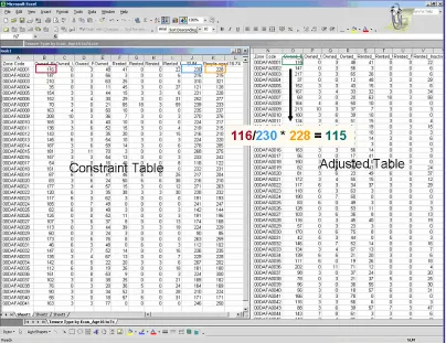
5.2 Input Adjustment

Given the problems mentioned above, it is therefore necessary to adjust the ‘Group Number’ and the constraint tables before using them. It should be noted that there is no way of deriving a true estimate of the number of residents or households prior to the imposition of disclosure control. However it is possible to improve on the method by extending the search for the same variable totals to tables in different datasets.

There are two steps needed to adjust the constraint tables. First is to adjust the ‘Group Number’ (number of people in the small areas that we want to populate). To do this the mean value of all related tables is used to give the number of people aged 16-74 in households for each small area. Secondly, each table cell is adjusted such that the row totals match these means.

The number of people in each cell is given by

Number of people from the constraint table x Group Number

Figure 5 shows the (original) constraint table from the census on the left and the adjusted constraint table on the right. The number of people for output area 00DAFA0001 in the adjusted table is 115, which is derived from 116 divided by the total sum of people in that area (from the constraint table) and multiplied by the ‘Group Number’.

As can be seen we attempt to minimise discrepancies between the totals of the constraint tables using this method. Although the adjusted tables may not be more accurate than the original CAS table, the adjustment method ensures the constraint tables are more consistent or at least can be guaranteed to produce the smallest discrepancy. Despite this, a rounding error of up to + 5 can be expected.

5.3 Model Execution Process

The algorithmic steps of the Simulated Annealing-Based Reweighting Program are as follows:

Step 1: Read in model file

Step 2: Read in constraint tables and microdata records referenced in the model file.

Step 3: Query the microdata according to the definitions in the model file

Step 4: Select sufficient individuals at random to populate the tables.

Step 5: Apply simulated annealing to find the best fitting set of individuals by the step 3 query result.

Step 6: When error = 0 or iteration count is exceeded then write out the best set of

records.

Clearly, the program starts by reading in the model file (see Appendix) which contains the path to all input datasets. Then the constraint table files are read in followed by the microdata file and the ‘Group Number’ file. The first key part of the program is the ‘microdata filtering process’. During this process the algorithm goes through the entire microdata database and checks whether an individual potentially fits into each column of the constrainting tables for the current area. This operation essentially links variables in one dataset to similar, but not identical, variables in another dataset. The filter queries the microdata by using logic operations and conditions including:

- OR

- AND

- OR NOT

- AND NOT

- =

For example, for the column of ‘Rented_1Car_Employed’ (people who are employed living in rented house and have 1 car) the following variables were queried.

Where:

TENHARM is tenure type (2=Social rented sector; 3=Private rented sector) REMPLOY is Employment status (1 = Employed)

NUMCARS is Number of Cars

INDIVI#DUAL is individual microdata

Another example is useful: for the column ‘Male_25-34_not couple’ the following variables were queried.

Where:

MARST is marital status (1 = Single, that is, never married, 3 = Married and separated from husband/wife, 4 = Divorced, 5 = Widowed)

SEX (1= male)

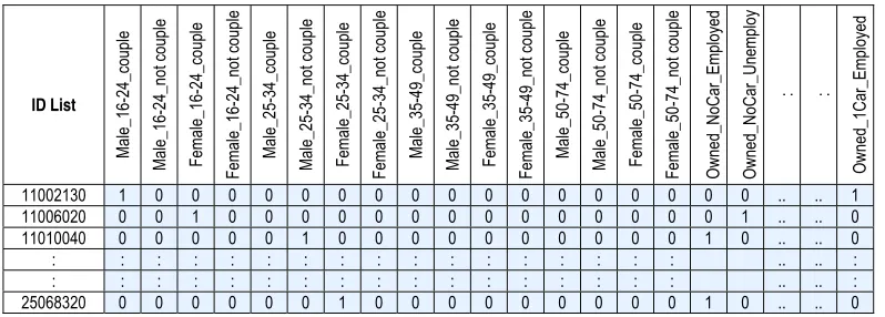
Through this process, we gain information as to whether the individuals fit each of the column constraints for all tables. Figure 6 shows the results of the ‘microdata filtering process’. Each individual is checked to see whether or not it fits the column constraints. If it fits the system returns 1, otherwise it returns 0.

Column&Name,Rented_1Car_Employed OR,TENHARM,=,2,INDIVI#DUAL OR,TENHARM,=,3,INDIVI#DUAL AND,REMPLOY,=,1,INDIVI#DUAL AND,NUMCARS,=,1,INDIVI#DUAL

Column&Name,Male_25-34_not couple OR,MARST,=,1,INDIVI#DUAL OR,MARST,=,3,INDIVI#DUAL OR,MARST,=,4,INDIVI#DUAL OR,MARST,=,5,INDIVI#DUAL AND,SEX,=,1,INDIVI#DUAL

Figure 6: The process to check each individual fits the column constraints

The second key part is the ‘simulated annealing process’. This searches for the best

combinations of individuals based on the result of the filtering process. It is used to swap out individuals until the microsimulated individuals match the aggregate area statistics for a variety of census data. A simple example can be described. Assume that if there are 200 people in a particular output area according to the census and 100 are females and the remaining 100 are males. The aim of simulated annealing is to find the set of people that best fit this sex constraint. To do this an initial random sample of records is selected from the BCS until sufficient individuals are represented (which is 200 in this example). Then, individuals are swapped to improve the match with the census statistics (male 100 and female 100). The ‘simulated annealing process’ is applied in an iterative manner. It is repeated with the aim of gradually improving the fit between the observed data and the selected combination of individuals from the BCS. A record is randomly selected and then replaced, with the replacement being kept if it improves the ‘error’ when compared with the constraint table. Each pair of tables is compared and the absolute error is calculated (Table 8 in section 6).

In particular, we adopted a similar methodology to SimLeeds2 used by Ballas (2001). SimCrime uses a similar object-oriented simulated annealing algorithm to minimise the difference between constraint tables from the 2001 Census Area Statistics and tables aggregated from synthetic microdata. In order to do this an initially selected individual is selected at random and replaced with one selected at random from the entire records. The error is recalculated and the change in error (Δe) is calculated. If Δe is less than zero, the change will be automatically accepted as an improvement. If not then, exp(-Δe/t) is compared to a random number between 0 to 1. If it is greater than the random number, the change is accepted; else the change is rejected and

2

A spatial microsimulation model that has been used to explore the potential spatial impact of a factory closure in Leeds at ward level, and to estimate the geographical impact of other national social policies (Ballas, 2001; Ballas and Clarke, 2001a, b)

ID List M al e_16-24_c oupl e M al e_16-24_not c ou pl e Fem al e_16-24_ coup le Fem al e_16-24_n ot c oupl e M al e_25-34_c oupl e M al e_25-34_not c ou pl e Fem al e_25-34_ coup le Fem al e_25-34_n ot c oupl e M al e_35-49_c oupl e M al e_35-49_not c ou pl e Fem al e_35-49_ coup le Fem al e_35-49_n ot c oupl e M al e_50-74_c oupl e M al e_50-74_not c ou pl e Fem al e_50-74_ coup le Fem al e_50-74_n ot c oupl e O w ned_N oC ar_E m pl oy ed O w ned_N oC ar_U ne m pl oy : : O w ned_1C ar_E m pl oy ed

11002130 1 0 0 0 0 0 0 0 0 0 0 0 0 0 0 0 0 0 .. .. 1

11006020 0 0 1 0 0 0 0 0 0 0 0 0 0 0 0 0 0 1 .. .. 0

11010040 0 0 0 0 0 1 0 0 0 0 0 0 0 0 0 0 1 0 .. .. 0

: : : : : : : : : : : : : : : : : .. .. :

: : : : : : : : : : : : : : : : : .. .. :

reversed. If Δe is 0 the change is accepted to allow the exploration of a greater part of the solution space. If the new error is the best seen so far the set of individuals is kept. The whole process is summarised in Figure 7. The process will continue until certain conditions (control parameters) are reached.

To find the best possible solution within available time the parameters must be carefully specified for the simulated annealing algorithm. These are an initial temperature, the percentage of temperature reduction each iteration, the number of iterations to be performed at each temperature step and a stopping criterion for the search.

The temperature plays an important role as a ‘control parameter’. It is initially set high and then slowly lowered. Master (1995) showed that at higher initial temperatures there are usually less iterations. When the temperature drops there are more iterations. In this study the algorithm begins with a very broad search area and the distance searched at the reduced new temperature will be less than its predecessor. But how quickly or how much should the temperature reduction be each time? It has been found that if the temperature drops too slowly a large amount of computation time may be required. If it drops too quickly we may not find the best solution because the fast reduction may be too confining (which can cause the algorithm to get stuck in a local minimum).

To run the Simulated Annealing-Based Reweighting Program these control parameters were set:

̇ Initial Temperature = 10,000

̇ Max Iterations = 10,000

̇ Dropping Percentage = 0.05

̇ Number of Model Restarts = 3 times (the ‘simulated annealing process’ is repeated three times and the best result is retained)

It should be noted that the Simulated Annealing-Based Reweighting Program is very

Input

People Aged 16-74 in HHs 3 Constraint Tables The BCS Microdata

Number of people _{16 categories} CS004 _{24 categories} CS061 _{18 categories} CS047 1,642 variables

2 ,4 3 9 O u tp u t A re a s

2,439 x 1 cells 2 ,4 3 9 O u tp u t A re a s

2,439 x 16 cells

2,439 x 24 cells

2,439 x 18 cells 3 2 ,8 2 4 i n d iv id u a ls

32,824 x 1,642 cells

Apply Simulated Annealing

A record is randomly selected and then replaced for the best error by comparing with the constraint table (Each pair of tables are compared and the absolute error will be calculated)

Rules

If the change in error (Δe) < 0 The change is accepted unconditionally (as an improvement). If exp(-Δe/ t) > random number (0-1) The change is accepted probabilistically

Else The change is rejected and reversed If the absolute error = 0 Stop searching

The process will continue until certain conditions are reached

Figure 7: SimCrime Framework

Output

List of Individuals (with the attributes) Aged 16-74 in Households

at Output Area Level Error Report by Output Area

514,523 individuals 2,439 Output

5.4 Model Output

The output from the Simulated Annealing-Based Reweighting Program comprises of two files:

1)

demographic and socio-economic characteristics. In addition, the attributes include victimisation-related variables from the 2001/2002 BCS. There are 514,523 individuals aged 16-74 in households in Leeds whose characteristics match the characteristics of the 514,523 individuals living in Leeds, as shown in the 2001 Census.

2)

between distributions of each constraint table and the synthetic microdata at the output area level. Each cell shows the absolute difference between the estimated and expected count (Table 8c).

Figure 8: Distribution of females single, widowed, or divorced aged 25-49 living

in rented house by output area in Leeds

Figure 9: Distribution of full-time students aged 20-30 living in rented

house by output area

Females SWD aged 25-49 in rented house 0

Figure 10: Distribution of high-class households with owner occupier

having at least 1 car

Figure 11: Distribution of males aged 16-24 unemployed and living in the

6.

Evaluation of Synthetic Microdata

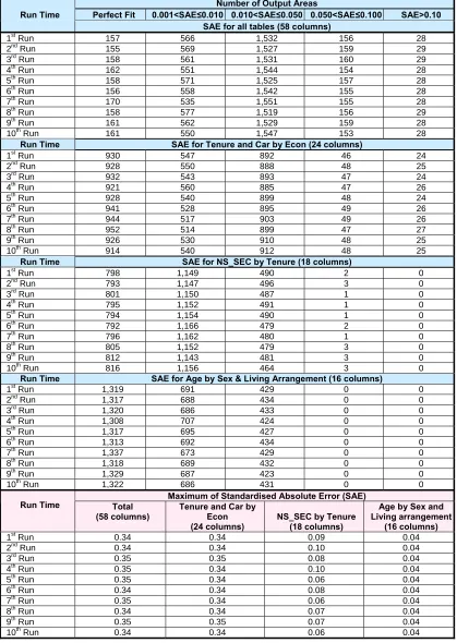
The objective of generating synthetic microdata is to generate data that does not currently exist for small areas. Therefore validation is difficult. This is one of the biggest drawbacks of the microsimulation framework. However, as Ballas (2001) pointed out, one way of validating microsimulation model outputs is to re-aggregate estimated datasets to levels at which observed datasets exist and compare the estimated distributions with the observed. The model outputs in this study are therefore evaluated in terms of their match to the constraint tables (socio-economic characteristics of individuals) from the census at the output area level.

The fit of a combination of individuals to known small area constraints is evaluated by the Total Absolute Error (TAE), the sum of the absolute differences between estimated and observed counts:

TAE = _{ij ij}

ij

T

U −

∑

Where

U

ij

T