A Two-phase Approach for Real-world Train Unit Scheduling

White Rose Research Online URL for this paper:

http://eprints.whiterose.ac.uk/74928/

Conference or Workshop Item:

Lin, Z and Kwan, RS A Two-phase Approach for Real-world Train Unit Scheduling. In:

Conference on Advanced Systems for Public Transport (CASPT12), 23-27 July 2012,

Santiago, Chile.

[email protected] https://eprints.whiterose.ac.uk/ Reuse

See Attached

Takedown

If you consider content in White Rose Research Online to be in breach of UK law, please notify us by

Zhiyuan Lin · Raymond S. K. Kwan

Abstract A two-phase approach for the train unit scheduling problem is proposed. The first phase assigns and sequences train trips to train units temporarily ignoring some infrastructure details at train stations. The solutions of the first phase would be near-operable. The second phase focuses on satisfying the remaining constraints with respect to detailed station layouts. Real-world scenarios such as compatibility among traction types and time allowances for coupling/decoupling activities are considered, so that the solutions would be fully operable.

The first phase is modeled as a large scale integer multi-commodity network flow (MCNF) problem. A branch-and-price integer linear programming approach is proposed. Preliminary ex-periments have shown that the approach would not yield solutions in reasonable time for problem instances exceeding about 1000 train trips. The train company collaborating in this research oper-ates over 2400 train trips on a typical weekday. Hence, a heuristic has been designed for compacting the problem instance to a much smaller size before the ILP solver is applied. The process is itera-tive with evolving compaction based on the results from the previous iteration thereby converging to near optimal results.

The second phase is modeled as a multidimensional matching problem with a mixed integer linear programming (MILP) formulation.

Keywords train unit scheduling · railway shunting · large-scale integer linear programming · column generation

1 Introduction

A train multiple unit, or train unit for short, is a set of train carriages with its own built-in engine(s), i.e. it is not pulled by a separate locomotive, and being able to move in both directions on its own. A train unit can also be coupled with other units of the same or similar types to increase the passenger carrying capacity or to redistribute the units across the rail network.Train unit scheduling refers to the planning of how timetabled train trips (or simply trains) in one operational day are sequenced to be operated by each train unit in the company’s fleet. Usually performed after the timetable has been fixed, and followed by a subsequent crew scheduling stage, train unit scheduling is also calledtrain unit diagramming where aunit diagram is a standardized documentation of the sequence of trains and other auxiliary activities, e.g. coupling and decoupling, an individual train unit will serve on a specified day of operation.

Z. Lin

School of Computing, University of Leeds, Leeds, LS2 9JT, United Kingdom Tel.: +44 (0)113 343 5430

Fax: +44 (0)113 343 5468 E-mail: [email protected] R. S. K. Kwan

School of Computing, University of Leeds, Leeds, LS2 9JT, United Kingdom Tel.: +44 (0)113 343 5430

Optimization in train unit scheduling is very important because of the high costs associated with leasing, operating and maintaining a fleet. It would also impact upon the subsequent planning of crew resources. For some heavily used commuter networks, e.g. in the North and South of Eng-land, train unit scheduling is also important for best distributing limited rolling stock resources, by coupling/decoupling train units and/or running them empty, to meet passenger demands. In real-world practice, there are often thousands of timetabled trains to be scheduled and complex rail infrastructure layouts, especially at large train stations, making train unit scheduling optimization a very hard problem to solve.

In this paper, a two-phase approach is proposed. The first phase is mainly a train sequencing and fleet assignment problem, leaving the resolution of how the train units would feasibly flow through the precise station layouts to the second phase. An integer multi-commodity network flow (MCNF) model similar to Cacchiani et al (2010), but more comprehensive in modeling the real-world conditions and constraints typical of UK rail operations, is used in the first phase. Fleet size and type constraints, linkage time allowance validity and coupling/decoupling possibilities are included in the model. The objective function minimizes a total weighted cost based on fleet size, operational costs, empty movement mileage, route preferences and a penalty measure of the extent to which the train capacity achieved is not meeting targets.

The second phase, as a railway shunting subproblem, finally determines the finer operational plan details. For example, precise track and platform layout constraints are considered. The shunt-ing (empty movements between platforms, sidshunt-ings and depots) subproblems are modeled as a mul-tidimensional matching problem, which eliminates “crossing” shunting movements and minimizes operational costs. The branch-and-price (Barnhart et al (1998)) approach, which has been suc-cessfully applied in solving large-scale integer linear programming (ILP) problems, will be used. In applying branch-and-price, the alternatives of column generation by means of either solving a sub-problem dynamically or selecting from a vast pre-generated set are compared.

The remainder of this paper is organized as follows. Section 2 introduces the train unit schedul-ing problem and highlights some aspects and features that are essential or important in the UK railway industry. Section 3 gives a brief overview on relevant literature. Section 4 and 5 present the two-phase approach models. Section 6 describes the methods for solving the proposed models. Finally Section 7 draws conclusions and remarks on the ongoing testing, with collaboration with Southern Railway, UK, and further research.

2 Problem Description

Given a set of fixed trains in a railway operator’s daily timetable, and a fleet of train units of different types, the train unit scheduling problem aims at determining an assignment plan such that each train is appropriately covered by a single or coupled units, with certain objectives achieved and certain constraints respected. From the perspective of a train unit, the scheduling process assigns a sequence of trains to it as its daily workload (forming a unit diagram). Maintenance provision can often be achieved either within the slacks in the diagrams or by swapping physical units assigned to the unit diagrams (Mar´oti and Kroon (2005)), thus maintenance planning is conventionally ignored at the stage of train unit scheduling.

The main objectives are to minimize the number of units used and/or the operational costs. It is also a common objective to meet the passenger capacity demands, which are often higher than the minimum capacity of individual units in the fleet, as much as possible.

2.1 Scheduling Constraints

The basic hard constraints for the schedule to be operable are:

(i) Each train must be served by at least one unit.

(iii) The sequence of trains assigned to a unit must be compatible in terms of the unit traction types and the routes traversed

(iv) The unit diagrams must not be in temporal or spatial conflict with each other. Such conflicts often arise from track and platform layouts at the train stations.

Some soft constraints are:

(i) Each train should be covered by atrain set of one or more units whose total capacity satisfies the passenger demand predicted for the train.

(ii) It is desirable to achieve some long gaps of appropriate time lengths between trains dur-ing certain times. Such long gaps in the unit diagrams would ease the subsequent task of maintenance planning.

(iii) Beyond mandatory compatibility between the trains sequenced together, there may be pref-erences for specific unit types and routes for individual trains

2.1.1 Coupling and Decoupling Activities

A challenging aspect of train unit scheduling is that sometimes more than one units can be assigned to cover the same train, known ascoupling(or attaching); the reversal activity is calleddecoupling (or detaching). Units of the same traction type (disregarding the number of carriages, which might be referred to as sub-types) can be coupled together, although a certain small number of different types may also be treated as compatible for coupling. The maximum number of units that can be coupled depends on many factors such as platform lengths and traction types. There are also restrictions on where coupling/decoupling activities are permitted to take place.

Coupling/decoupling activities are often essential to satisfying passenger demands. However, the time allowances required (typically 2 to 5 minutes) for accomplishing such activities may hinder the overall schedule efficiency to some extent, and add to the complexity of the scheduling problem. Moreover, after having provided the required passenger carrying capacity, some coupled units would inevitably have been displaced to parts of the network that become in excess in terms of capacity provision, and they would have to be redistributed to other locations by coupling, serving trains that do not need the extra capacity, or by empty running.

Coupling/decoupling sometimes is not restricted to take place at the beginning/end of a train trip. That is, train units may be joined or split en-route. These scenarios are often related to the topological structure of the railway network, e.g. hubs and junctions. Passengers would have to pay attention as to which carriages are associated with which destinations. Mar´oti (2006) refers to these special cases of coupling/decoupling as “joining/splitting”.

For a set of coupled units (a unit block), not only its composition is important, but also its permutation/order of units. The reason is that sometimes coupling/decoupling can only be performed in certain order; it may also cause issues like blockage in shunting movements.

Although appropriate coupling/decoupling activities may contribute to an optimal schedule, they would also consume resources like tracks, shunting operations, crew and time. It is therefore important to avoid unnecessary coupling/decoupling activities. Sometimes, it may be preferable to keep a unit block together for longer rather than reversing the coupling/decoupling actions between the units in the block several times.

2.1.2 Empty Running

An advantage of relocating a train unit by means of coupling onto another unit serving a timetabled train trip is that there would not be any conflicts in terms of track usage, and therefore eases the scheduling process. On the other hand, running a unit empty, i.e. without passengers, may be more flexible in terms of its timing. The disadvantages are that the path and timing of an empty train has to be checked and approved to ensure that it is not in conflict with other track users; and that the empty running is not directly contributing to passenger carrying capacity. Also, empty runnings have significant additional operational costs.

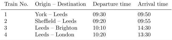
Table 1 Example trains at the same platform

Train No. Origin – Destination Departure time Arrival time

1 York – Leeds 09:30 09:50

2 Sheffield – Leeds 09:20 09:55

3 Leeds – Brighton 10:10 14:30

4 Leeds – London 10:20 13:30

In an automatic scheduling process, empty running is usually planned using a predefined collection of empty running journey time allowances between location pairs. There may also be time zones when empty running is prohibited. At the end of the scheduling process, empty running trains are planned in detail and ensured to be conflict free. At that stage, it is possible that some adjustments to the schedule are required because some empty runnings turn out to be infeasible.

2.1.3 Shunting Movements and Infrastructure

The linkage between an arriving train and a departing train sometimes may only be accomplished by certain shunting movements. Railway shunting generally refers to empty-running movements betweenplatforms,sidingsanddepotsduring a linkage. Shunting plans enable units to be delivered to the right location at the right time without causing blockage to each other. The length of empty running required varies between different types of shunting movement. Whereas the arrival and departure platforms for trains are usually assigned at the timetable planning stage, the assignment of which sidings or depots the units will be shunted to are only planned at the unit diagramming stage. Since depot shunting usually occurs before or after an idle period for the unit, it is generally less constraining on unit scheduling.

A distinctive feature that makes rolling stock scheduling different from road (e.g. bus) vehicle scheduling is that movements of rolling stocks are strictly restricted by tracks and other railway infrastructures like platforms and sidings, giving additional problems such as unit blockage or hitting platform or siding capacity restrictions. In some literature, blockage is also known as crossing (Freling et al (2005), Kroon et al (2008)). Other issues may also be relevant to shunting, for example, compatibility between traction type and platform/siding/depot.

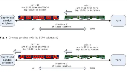
To illustrate how crossing can invalidate a unit diagram derived solely based on timetable and fleet information (i.e. without infrastructure information on track layouts etc.), consider a simple example. Table 1 gives a timetable of four trains. Suppose at Leeds Station all the four trains have been assigned to the same platform, where the tracks arebidirectional – i.e. both “up” and “down” movements are allowed. There are two train units available each with sufficient capacity for any of the trains. Suppose Unit I can only serve Trains 1, 3 and 4, while Unit II can serve Trains 2, 3 and 4.

Applying the FIFO rule matching arrivals to departures at the platform would give the fol-lowing solution:

(i) Unit I: Train 1−→Train 3, Unit II: Train 2−→Train 4;

But solution (i) is infeasible because when departing at 10:10, Unit I will be obstructed by Unit II whose departure time is 10:20. It would be easy to see that an alternative feasible solutions exists:

(ii) Unit I: Train 1 −→Train 4, Unit II: Train 2−→Train 3.

The two solutions are illustrated in Figure 1 and 2, illustrating how train directions and infrastructure can seriously affect the results if the scheduling process does not take them into consideration.

Fig. 1 Crossing problem with the FIFO solution (i)

Fig. 2 A feasible solution (ii)

depots. High-level planning alone may result in problems such as crossing, which would hinder the solutions from being operable; but then, incorporating every detailed infrastructure information into the scheduling algorithm will lead to an extremely huge-sized optimization problem instance intractable to solve. Therefore, a two-phase approach is preferred as a compromise, which is to be discussed in Section 4 and 5.

3 Literature Review

Our discussion will focus on each of the two phases of the proposed approach as well as solving large-scale integer linear programs.

3.1 Train Sequencing and Fleet Assignment Problem

Bodin et al (1983) give a general survey on vehicle scheduling. Mar´oti (2006) and Cacchiani et al (2010) have reviewed relevant railway scheduling problems. Researches specifically on train unit scheduling are relatively few. In this section, we shall focus on the sequencing/circulation aspects, shunting and infrastructure related research will be discussed in the next section.

Schrijver (1993) proposes a multi-commodity circulation flow model concerning the rolling stock scheduling problem for a single line and a single day for NS Reizigers with about a hundred train trips; the objective is to minimize the total number of train units used. Passenger capacity demands, maximum number of units coupled, multiple types of train unit and cycling/maintenance are considered. Other coupling/decoupling and shunting/infrastructure restrictions are ignored. Some polyhedral techniques are used to speed up the solution process.

Fioole et al (2006) describe a similar model and instance as Alfieri et al (2006) with additional considerations on train splitting and joining. Peeters and Kroon (2008) describe a similar model and instance as Alfieri et al (2006) with a specialized solver employing branch-and-price.

Mar´oti (2006) proposes generalized models of the above works in the Netherlands in his PhD thesis.

More recently, Cacchiani et al (2010) propose an integer MCNF model solved by column generation with shortest path subproblems including some heuristic methods to improve efficiency. This model takes considerations of coupling/decoupling and vehicle-route compatibility, and is reported to have been applied for real-world instances of up to 600 train trips. Coupling/decoupling time allowances, traction type compatibility and shunting restrictions do not seem to have been considered in the model.

3.2 Railway Shunting Problem

Freling et al (2005) propose a two-phase approach to solve the railway shunting problem at a station within a 24-hour horizon. The first phase consists of matching arrival units to departure units such that blocks of linked units are generated; the second phase assigns the unit blocks to appropriate sidings. The method is based on a set-partitioning ILP model with each column corresponding to a feasible assignment plan for a siding. Both single (FILO) and double (free) sidings are considered. It prevents overcapacity and crossing at each siding, and also minimizes unnecessary coupling/decoupling activities. The instances tested have up to about 80 train units to be parked at 19 sidings. This two-phase approach gives near- optimal solutions, and the gap from global optimality seems to be small as reported.

Kroon et al (2008) later propose another approach for the same railway shunting problem as in Freling et al (2005), where an integrated model (and three of its variants) is devised such that matching and assigning is processed together, hence global optimality is guaranteed. This model uses a 3-dimensional matching formulation, requiring a reasonable amount of computation time to obtain high quality results such that unnecessary coupling/decoupling is minimized and units of the same type are encouraged to be parked at the same siding. To avoid a possible huge number of crossing constraints, maximal cliques and comparability graph techniques are used. Some heuristics are also employed, for example, taking advantage of homogeneous sidings to reduce crossing constraints.

Cardonha and Bornd¨orfer (2009) propose a novel set-partitioning model and an associated column generation approach for a generalized vehicle shunting problem. The model provides a tight linear description of the problem and can, in particular, produce non-trivial lower bounds. The pricing problem, and the LP relaxation itself, can be solved in polynomial time, for some versions of the problem.

3.3 Solving Large-scale Integer Linear Programs

3.3.1 Branch-and-price and Integer Multi-commodity Network Flow Problem

3.3.2 Generate-and-select and PowerSolver

Dynamic column generation needs a fast non-enumerative pricing algorithm. However for real-world applications, the pricing subproblems are often computationally expensive for even mod-erately large problem instances. Kwan (2004) presents aGenerate-and-Select (GaS) approach in crew scheduling, in which the column generation process only brings in new columns within a pre-generated very large collection of columns. Apart from the advantage of reducing computa-tion associated with solving pricing subproblems, a reasonably sized seleccomputa-tion of the pre-generated columns could also be made for the branch and bound process seeking integer solutions. Kwan and Kwan (2007) further propose a hybrid method calledPowerSolver to solve very-large-scale train crew scheduling problems. PowerSolver uses an iterative heuristics to control the size of the problem instance in each execution of its core algorithm (GaS with set-covering ILP) such that the ILP solver works comfortably due to the reduced problem size. Initially, the controlled problem instance is a crude simplification of the original problem instance; it is then refined and converges to containing the crucial features in a compact form over a number of iterations. A mechanism to ensure that new solutions would not be worse than the current best is embedded, thus the results would converge to a near-optimal one within a relatively short time. PowerSolver is now part of the TrainTRACS system (Fores et al (2002); Wren et al (2003)) and is proving successful by many UK transport operators who are now routinely using it. A similar approach to PowerSolver could be applied in train unit scheduling and will be discussed in later sections.

4 A Multi-commodity Flow Model for the First Phase

Considering that the unit scheduling problem would be huge and intractable if all detailed infras-tructure constraints are to be considered at once, a two-phase approach is proposed.

The first phase for train sequencing and fleet assignment uses an MCNF model similar to Cacchiani et al (2010). But the model is more comprehensive in modeling real-world conditions and constraints typical of railway operations, especially the coupling/decoupling time allowance constraints and type compatibility constraints. The aim is to produce solutions that are near to being fully operable. The objective function minimizes a total weighted cost based on fleet size, operational costs, empty movement mileage, route preferences, idle time and a penalty measure of the extent to which the train capacity achieved is not meeting targets.

The second phase (railway shunting) finally determines the finer operational plan details in a station-by-station manner. For example, precise track and platform layout constraints are consid-ered for determining the best operable shunting movement plans. It will be described in Section 5.

4.1 Model Description

The MCNF model is based on a framework ofdirected acyclic graph (DAG) representing trains and their linkage relations. A generic DAG G= (N,A) consists of nodes and directed arcs such that no cycle exists.

In this framework, the majority of nodes represent the trains in the timetable, thus are called train nodes. In addition, asource node 0 and a sink node ∞are added as usual. There are three kinds of arcs in the DAG, namelysign-in arcs,sign-off arcs andlinkage arcs. A sign-in arc starts from the source node and terminates at a train node; a sign-off arc starts from a train node and terminates at the sink node. Generally all train nodes have a in arc coming into it and a sign-off arc leaving from it. A linkage arca links two train nodes i andj (a= (i, j)), representing a potential link, with a sufficient time gap, such that after serving trainia unit block with permitted type(s) can continue to serve trainj as its next task. Apath in the DAG is defined as a sequence of nodes starting from the source to the sink such that from each of its nodes there is an arc to the next node in the sequence. A path represents the daily workload (a diagram) for a unit.

Table 2 describes the symbols representing entities in the DAG.

In order to deal with type-route compatibility, type-graphsGt _{(are also DAGs) representing}

Table 2 DAG entities

Symbols Entities in the DAG 0 the source node

∞ the sink node

i, j, ... nodes

N set of all nodes

N◦_{={0,∞} set of source and sink nodes}

e

N set of train nodes

aor (i, j) an arc

A set of arcs

δ−(j) set of in-flow arcs of nodej δ+(j) set of out-flow arcs of nodej

A◦ _{set of sign in and off arcs}

e

A set of linkage arcs

v−(a) start vertex (node) of arca v+(a) end vertex (node) of arca

E ⊂Ae set of all empty-running trains (represented by the arc containing it)

E†_{(a)⊂Ae set of all conflicting empty-running trains of empty-running train inside arca} p a path

P set of paths

Pj set of paths passing through nodej

Pa set of paths passing through arca

Jp set oftrainnodes in pathp t a unit type

T set of all unit types

f a unit family (see Section 4.2)

F set of unit families (see Section 4.2)

Table 3 Parameters

Symbols Meaning

Wi, i= 1,· · ·,8 weights of terms in the objective

µt

j mileage of trainjused by typet(not including empty-running trains) γt

a a binary indicator showing whether arcais a long gap for typet πt

j weight for the preference of type-train pair (t, j): the higher, the more suitable πt

a weight for the preference of type-sign-in/off arc pair (t, a), a∈ A◦: the higher,

the more suitable

Ft upper bound of fleet size of unit typet Ft _{lower bound of fleet size of unit typet} κt _{unit capacity of typet}

r_j hard (lower) passengers’ demand for trainj rj soft (upper) passengers’ demand for trainj

U_jf maximum number (in cars or units) of familyf∈ F coupled at trainj νt _{number of cars of unit typet}

lt _{length of unit typet}

Lj:= min{Ldep(j), Larr(j)} the minimum length between departure platform and arrival platform of train

j τC

dep(j) single coupling time at the departure platform of trainj

τD

arr(j) single decoupling time at the arrival platform of trainj

eij spare time in linkage arc (i, j) ∈ Ae, used for time allowance validity for coupling/decoupling activities

Ma the possibly largest number of coupled units at arca

All entities in the type-graphsGt_{can be symbolized by adding atsuperscript in the corresponding}

notations of the complete DAGG, e.g.Pt_{refers to set of all paths in type-graphG}t_.

Table 3 describes the parameters used in the model.

A path pin a type-graphGt_{of type t (denoted asp∈ P}t_{) represents a sequence of trains to}

be covered by a unit or units of typet (if the latter case, it means the units are coupled together throughout the day). Also, if more than one flow/selected path share a common train node, it means this train is covered by a unit block coupled by the units from those paths. A variable xp ∈ Z+ is used to indicate the number of unit(s) of type t used to serve the trains in path

p∈ Pt_{. Moreover, family-train indicator variable y}f

j∈Ne is served by a type from familyf (see Section 4.2); it can be used to calculate the existence of specific types in a coupled block such that incompatible types cannot be coupled. Blockflow variable za ∈ {0,1} is used to indicate whether an arc a = (i, j) is used. It is a block of units

that remains coupled together during two consecutive trainsi and j. za is used to calculate the

time consumed by coupling/decoupling operations; it can also be used to eliminate unnecessary coupling/decoupling activities at each station.

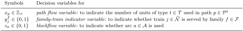
Table 4 describes the decision variables used in the MCNF ILP model.

Table 4 Decision variables

Symbols Decision variables for

xp∈Z_{+ path flow variable: to indicate the number of units of typet∈ T used in pathp∈ P}t yf_j ∈ {0,1} family-train indicator variable: to indicate whether trainj∈Ne is served by familyf∈ F

za∈ {0,1} blockflow variable: to indicate whether arca∈ Ais used

4.2 Some Issues on Coupling/Decoupling

4.2.1 Restricted Locations for Coupling/decoupling

This can be achieved by setting the single coupling/decoupling operation time of that location (usually a platform) into a very big number, e.g.τC

dep(j):=M, τarr(i)D :=M, then such operations

are prohibited at those locations (cf. Eq. (1)).

4.2.2 Time Consumed by Coupling/decoupling in a Linkage

Associated with an arc joining two train nodes, it is not possible to predetermine the amount of time required for coupling/decoupling activities because how many units flowing through the nodes are variable. The remedy is to use the block flow variableza, a∈Aeat each linkage arca

with the constraints below:

τ_dep(i)C



 X

a∈δ−(i) za−1



+τ_arr(j)D



 X

a∈δ+(j) za−1



≤eij, ∀(i, j)∈A;e (1)

4.2.3 Platform Lengths

There is an upper bound on the number of units that can be coupled in serving a train trip due to limited platform lengths, which can be achieved by the following constraints on each train node:

X

t∈T X

p∈Pt j

ltxp≤Lj:= min{Ldep(j), Larr(j)}, ∀j∈Ne; (2)

4.2.4 Type-type Compatibility

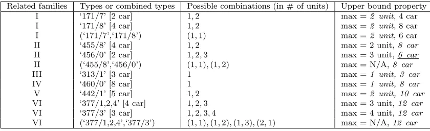
Coupling upper bound with respect to unit type is complicated by type-type compatibilities. In order to let these compatibilities be consistent with their varied coupling upper bounds, we introduce the concept oftrain unit family. Table 5 shows all possible combinations of unit types that can be coupled from the entire Southern Railway fleet based on different coupling upper bounds.

– Family I ={‘171/7’, ‘171/8’}

– Family II ={‘455/8’, ‘456/0’}

– Family III ={‘313/1’}

– Family IV ={‘460/0’}

– Family V ={‘442/1‘}

– Family VI ={‘377/1’, ‘377/2’, ‘377/3’, ‘377/4’}

Notice members in Family II actually do not share a common upper bound. Nevertheless, this can be remedied by adding extra constraints limiting the number of coupled 456/0 units to be no greater than 6. For each family, we set binary decision variablesyf_j ∈ {0,1},∀f ∈ F to indicate whether a trainj is served by any units from familyf. Then, incompatible types are excluded by the following constraints forcing only one family inF to serve a train:

X

f∈F

y_jf= 1, ∀j∈Ne. (3)

Then the upper bound constraint can be written as

X

f∈F1

X

t∈f X

p∈Pt j

νtxp+ X

f∈F2

X

t∈f X

p∈Pt j

xp≤ X

f∈F1

U_jfyf_j + X

f∈F2

U_jfyf_j, ∀j∈Ne, (4)

whereνt _{is the number of cars for typet andU}f

j is the upper bound in number ofunits orcars

familyf can be used to serve train j. The reason why this parameter is devised as U_jf (rather thanUf_{) is that a small proportion of this upper bound with respect to families can change on}

certain routes. For instance, Family I of diesel fleet British Rail Class ‘171/7’ and ‘171/8’ can generally be coupled up to a 2-unit block, however on the route from Ashford to Hastings, this upper bound is reduced to only 1 unit. Finally,F1 is the set of families sharing common upper

bounds in car number, andF2is the set of families sharing a common upper bound in unit number.

The parameterU_jf, f ∈ F1,2 will be set with a car number or unit number accordingly.

4.3 Path Formulation

If column generation is to be used for an MCNF problem, generally a path formulation would be preferred than an arc formulation. The LP-relaxations of the two formulations are equivalent (Cook et al (1998); Cacchiani et al (2010)). We choose an LP-relaxation rather than a Lagrangian relaxation as nowadays a state-of-art simplex solver can be more efficient than a subgradient method.

The path formulation:

Table 5 Unit type combinations and families of Southern Railway, UK

Related families Types or combined types Possible combinations (in # of units) Upper bound property I ‘171/7’ [2 car] 1,2 max =2 unit, 4 car I ‘171/8’ [4 car] 1,2 max =2 unit, 8 car I (‘171/7’,‘171/8’) (1,1) max =2 unit, 6 car II ‘455/8’ [4 car] 1,2 max = 2 unit,8 car

II ‘456/0’ [2 car] 1,2,3 max = 3 unit,6 car

II (‘455/8’,‘456/0’) (1,1),(1,2) max = N/A,8 car

III ‘313/1’ [3 car] 1 max =1 unit, 3 car

IV ‘460/0’ [8 car] 1 max =1 unit, 8 car

V ‘442/1’ [5 car] 1,2 max =2 unit, 10 car

VI ‘377/1,2,4’ [4 car] 1,2,3 max = 3 unit,12 car

VI ‘377/3’ [3 car] 1,2,3,4 max = 4 unit,12 car

min

x,z W1

X

t∈T X

p∈Pt

xp+W2 X

t∈T X

j∈Net

X

p∈Pt j

µt_jxp+W3 X

t∈T X

a∈Et

X

p∈Pt a

xp

−W4 X

t∈T X

a∈Aet

X

p∈Pt a

γ_atxp+W5 X

j∈Ne

X t∈T X

p∈Pt j

κtxp−rj

−W6 X

t∈T X

j∈Net

X

p∈Pt j

π_jtxp−W7 X

t∈T X

a∈(A◦₎t

X

p∈Pt a

πt_axp+W8 X a∈A za (5) subject to X

p∈Pt

xp≥Ft, ∀t∈ T; (6a)

X

p∈Pt

xp≤F t

, ∀t∈ T; (6b)

X

t∈T X

p∈Pt j

κtxp≥rj, ∀j∈Ne; (7)

y_jf≥ 1 U_jf

X

t∈f X

p∈Pt j

xp, ∀j∈Ne,∀f ∈ F1; (8a)

y_jf ≥ 1 U_jf

X

t∈f X

p∈Pt j

νtxp, ∀j∈Ne,∀f ∈ F2; (8b)

X

f∈F

y_jf= 1, ∀j∈Ne; (9)

X

f∈F1

X

t∈f X

p∈Pt j

νtxp+ X

f∈F2

X

t∈f X

p∈Pt j

xp≤ X

f∈F1

U_jfyf_j + X

f∈F2

U_jfyf_j, ∀j∈Ne; (10)

X

p∈Pt j

xp≤3, ∀j ∈Net, t= ‘456/0’; (11)

X

t∈T X

p∈Pt j

ltxp≤Lj, ∀j∈Ne; (12)

za≥

1 Ma

X

t∈T X

p∈Pt a

xp, ∀a∈A;e (13)

τdep(i)C 

 X

a∈δ−(i) za−1



+τarr(j)D 

 X

a∈δ+(j) za−1



≤eij, ∀(i, j)∈A;e (14)

za+

1 |E†_(a)|

X

a′_∈E†_(a)

za′ ≤1, ∀a∈ E:E†(a)6=∅; (15)

xp∈Z+, ∀p∈ Pt,∀t∈ T, (16a)

y_jf ∈ {0,1}, ∀j∈Ne, ∀f ∈ F, (16b)

4.3.1 Objective Function

The objective (5) is formed by a linear combination of eight terms. The first term minimizes the total number of units used. The second term minimizes the total passenger train unit-mileage, where µt

j is the mileage of trainj ∈Ne used by single unit of type t. The third term minimizes

the total number of empty-running trains. The fourth term encourages insertion of long gaps in unit diagrams such that maintenance can be realized whereby. Parameterγ_at= 0 if arcadoes not imply a long gap or this gap is not suitable for typet; γat >0 if arc acontains a long gap that

is suitable for typet. There are also preferences among positive values of γt

a as some long gaps

are more suitable for typet than others. The fifth term tries to minimize the summed deviation between actual unit capacity and upper demand per train. The nonlinearity caused by absolute value can be eliminated by adding extra variablesd+_j, d−_j ∈R_{+,∀j ∈N}e _{with constraints}

X

t∈T X

p∈Pt j

κtxp−rj =d+j −d−j , ∀j ∈Ne, (17)

and replacingP_t∈T P_p∈Pt jκ

t_x p−rj

in the objective by d+_j +d−_j. The sixth term encourages type-train (route) preferences, where πt

j ≥ 0 is a preference weight for a type-train pair (t, j):

the higher, the more suitable. The seventh term encourages sign-in/off arc preferences (usually related to home depots) for each type of units, wherepit

a stands for a preference parameter for

a type-sign-in/off arc pair (t, a): the higher, the more suitable. Notice if a certain type t is not suitable for a sign-in/off arc, then this arc will have not been not inserted into Gt _{in the first}

place. The eighth term minimizes the total number of blocks leading to minimization of the total number of coupling/decoupling activities; it also partly drivesza to desired binary values.

4.3.2 Constraints

Constraints (6) ensure the deployed number of units for each type is within a lower and an up-per bound. Constraints (7) guarantee satisfaction of a minimum level of capacity demand for each passenger train. Constraints (8) calculate each family-train indicator variable, and con-straints (9) allow only one family to serve a train. Notice (8) and (9) together will ensure that

yf_j =

(

1,P_t∈fP_p∈Pt jxp>0

0,P_t∈fP_p∈Pt jxp= 0

,∀j ∈ Ne,∀f ∈ F. Constraints (10) forbid the number of

cou-pled units exceeding certain upper bounds respect to trains and families. Constraints (11) are to modify (10) for the exceptional case of type 456/0. Constraints (12) are maximum platform length constraints. Constraints (13) calculate blockflow variables. Notice as the sum of blockflow

variables is minimized in the objective, the relation za =

1,P_t∈T P_p∈Ptxp>0

0,P_t∈T P_p∈Ptxp= 0

,∀a ∈ A is

guaranteed. Constraints (14) are to ensure time allowance validity for coupling/decoupling time. Constraints (15) are to exclude all conflicts among empty-running trains. Finally (16) forces the variables to be integral or binary.

5 A Multidimensional Matching Model for the Second Phase

5.1 Station Element Representation and Model Description

5.1.1 Arrival and Departure Units

The first phase provides a tentative schedule based on which the second phase operates within the scope of each individual stationσ∈Σ. The first phase fixes the unit-type assignment to each arrival and departure train, e.g., “train 1E08 is served by one British Rail Class 171/7 and one British Rail Class 171/8 units”. We can thus define a set of arrival units and a set of departure units for a day’s operation at each station σ, as u1, u2,· · · , un ∈ Uσ and v1, v2,· · · , vn ∈ Vσ

every arrival unit, and these assignments may have to be modified by the second phase because of operational conflicts at the station. Here we assume empty running trains have been inserted by the first phase and|Uσ_|=|Vσ_{|=n. Sign-in/off trains from/to a home depot can be dealt with by}

slight adaptation. Exceptions, such as over-night units remaining at the station cannot invalidate this model as sign-in/off arcs regard this station as the source/sink node. For simplicity reason, we will omit the superscriptσin later part of this section as everything is clearly based on a station, except where explicitly stating the station is necessary.

The attributes of each arrival and departure unit include:

– The train the unit belongs to: T(u), T(v). Notice an arrival unit only belongs to an arrival train and a departure unit only belongs to a departure train.

– The attributes due to its train: the arrival platform of an arrival unitP(u) and the departure platform of a departure unitP(v); the arrival time of an arrival unitτ(u) and the departure time of a departure unitτ(v).

– The type of that unit:t(u), t(v).

Amatching between an arrival unit and a departure unit is used to represent a linkage relation. A matching between twoconceptual arrival and departure units u and v indicates they will be materialized by being assigned to be the same unit. The first-step rule of how an arrival unit u can be matched with a departure unitvis: (a) Same type:t(u) =t(v); (b) the arrival time ofuis appropriately earlier than the departure time ofv:τ(u)≺τ(v).

Other linkage time validity rules regarding shunting/coupling/decoupling times will be consid-ered respectively in other ways. It is important to note that anappropriate matching between a pair of arrival and departure units (u, v), u∈ U, v∈ Vwill correspond to one and only one linkage arc (T(u), T(v))∈Aein the DAG defined in the first phase. This linkage arc is called a dominant arcof the matching pair.

5.1.2 Unit Position

If a train is a coupled one, thepositionsof the units in the coupled formation are significant. Since the first phase has not provided anything on unit permutation for coupled trains, the position attributes have to be decided in the second phase. Letp∈ Pu, q∈ Qv denote positions and their

possible choice sets for arrival unituand departure unitv respectively. For a unit u(orv) from a non-coupled train, its position has been decided a priori (|Pu|= 1 or |Qv|= 1); for a coupled

single-type (homogenous) train, unit positions can be pre-assigned based on the first phase result in an arbitrary order without losing any generality, leading to |Pu| = 1 or |Qv| = 1 as well;

for a coupled multi-type (heterogenous) train where different permutations can have essentially different results, a decision has to be made fromp∈ Pu, q∈ Qv,|Pu| ≥1,|Qv| ≥1. Therefore, the

above matching has to be further modified within apositioned pair of (u, p) and (v, q) such that a plan (u, p, v, q), u∈ U, p∈ Pu, v∈ V, q∈ Qv has to be made.

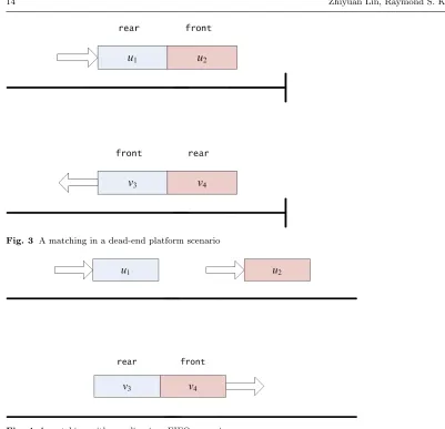
Unit permutation can significantly affect a schedule without infrastructure details. Figure 3 shows two arrival unitsu1, u2coupled in a train arriving at a dead-end platform, also two departure

unitsv3, v4coupled in a later departure train at the same platform suitable to be linked with the

arrival train. Suppose all the units have the same traction type and their positions have been pre-assigned as indicated in the figure. Without unit position and platform layout knowledge, it seems that any arrival unitsui, i= 1,2 can be matched with any departure unitsvj, j= 3,4. But

in factu1can only be matched withv3andu2withv4. Figure 4 gives another example concerning

arrival unitsu1, u2 and departure unitsv3, v4, suppose they all have the same traction type and

are at the same FIFO platform. Suppose their positions have been pre-assigned as indicated in the figure. Moreover,T(u1)6=T(u2) but T(v3) =T(v4) andτ(u1)≺τ(u2)≺τ(v3) =τ(v4) such

that the two arrival units can be coupled to serve the departure train. Here as the arrival train T(u2) comes earlier than T(u1) in a FIFO track, thenu1 can only be coupled at the rear ofu2,

which indicatesu1 can only be matched withv3and u2 withv4. The cases in coupled multi-type

Fig. 3 A matching in a dead-end platform scenario

Fig. 4 A matching with coupling in a FIFO scenario

5.1.3 Parking Berths

As discussed in Section 2.1.3, there are three possible kinds of shunting plans at each linkage arc: to let the unit continue to serve the next train within the platform area (short time gap linkage), to put the unit to a siding temporarily until it is needed for the next train (medium time gap linkage) and to put the unit to a nearby depot until it is needed for the next train (long time gap linkage). Here we denoteparking berths asb∈ B :={0} ∪ S ∪ D where 0 refers to a dummy parking berth,S the siding set andDthe depot set.

For a positioned pair of arrival and departure units (u, p, v, q), u∈ U, p∈ Pu, v ∈ V, q ∈ Qv,

the possible choice for parking berth types (dummy, siding or depot) is dependent on the relevant time gap length of its dominant linkage arc. A dummy berth is only imaginary, i.e. the unit stays put. However, if the parking berth turns out to be a siding or a depot, usually there are a number of sidings or depots available for a unit to be shunted to. We denote the possible parking berths for a pair of positioned units (u, p, v, q) asB(u, p, v, q).

5.1.4 Parking Methods

In order to avoid crossings, the way a unit comes to/leaves a platform or a siding should be taken into account. It is usually not important how a unit comes to/leaves a depot after an empty-running trip. This is because such movements are usually infrequent with much slack time available for resolving any conflicts that might arise.

arrival platformP(u), comes to and leaves its parking berthb, and then comes to and departs from the departure platformP(v). For a pair yielding a dummy or a depot parking berthb∈ {0} ∪ D, the ways coming to and leavingbis omitted as a default “00”.

Here is an example of such a parking method withb= 0 and a null-shunting:m= [LR,00, LR], which means arriving from the left and departing from the right, at the same platform without any shunting. Another example of a parking method of a double (free) siding shunting with re-platforming:m= [LR, RL, LL] which means:

– at the arrival platform: arriving from the left and leaving from the right (to a siding);

– at the siding: coming from the right and leaving from the left (to the departure platform);

– at the departure platform: coming from the left and departing from the left.

Parking methods are determined by various factors, e.g. train directions, platform, unit po-sition, siding, depot and overall layout relations, plus possible engineering and operational regu-lations. Usually when (u, p, v, q, b) is fixed, the resulting M(u, p, v, q, b) would have a very small number of candidate methods. Especially when the parking berth is a dummy one, a single (FILO) siding or a depot, the possible parking method is very likely to be unique.

5.1.5 Shunting Plans and Conflicts between a Pair of Shunting Plans

The second phase shunting problem is defined as

At each station σ∈Σ of the rail network, give each arrival unit u∈ U a positionp∈ Pu and

assign it to a departure unitv ∈ V with position q∈ Qv, via a parking berth b∈ B(u, p, v, q) and

with a parking methodm∈ M(u, p, v, q, b)such that

1. Each matching pair (u, v)implies a dominant linkage arc relation(T(u), T(v))∈Ae; 2. Each positioned pair(u, p, v, q)is operationally feasible for connecting T(u)andT(v); 3. No crossing occur at platforms or sidings;

4. No overcapacity occur at any sidings or depots (already satisfied in the first phase);

5. No breaking on any other temporal, spatial, engineering or operational rules that makes the overall plan inoperable.

A shunting plan can be expressed as a 6-tuple (u, p, v, q, b, m), u ∈ U, v ∈ V,(T(u), T(v))∈

e

A, p ∈ Pu, q ∈ Qv, b ∈ B(u, p, v, q), m ∈ M(u, p, v, q, b) representing a self-consistent shunting

plan. For convenience, a shunting plan (u, p, v, q, b, m) can also be written as π ∈ Π when its details can be omitted, where we denote the set of all possible shunting plans at a station asΠ. The set of shunting plans all involving a specific arrival unit ucan be written as Πu, the same

forΠv for a specific departure unitv. Fig.5 gives an illustration of the concept of shunting plans

(unit positioning is not depicted).

All the possible shunting plans can be pre-computed based on input data of station information and the first phase results before the second phase begins. With a shunting plan (u, p, v, q, b, m) timings can be determined for the unit leaving the arrival platform, coming to the parking berth, leaving the parking berth and coming to the departure platform. Also, the following parameters are known from station layout knowledge.∆τu: time duration at the arrival platformP(u);∆τub:

shunting/empty-running time from platform P(u) to parking berth b; ∆τbv:

shunting/empty-running time from parking berthbto platformP(v);∆τv: time duration at the departure platform

P(v). Then, the attributes of a shunting plan (u, p, v, q, b, m) include:

– All attributes inherited from its arrival and departure units, including traction types, trains, positions and platforms;

– At the arrival platformP(u): arrival timeτ(u), leaving timeλ(u) :=τ(u) +∆τu, which forms

atime window at the arrival platform:Wu(u, p, v, q, b, m) := [τ(u), λ(u)];

– At the departure platformP(v): coming time:χ(v) :=τ(v)−∆τv, departure timeτ(v), which

forms a time window at the departure platform:Wv(u, p, v, q, b, m) := [χ(v), τ(v)];

– At parking berthb: coming timeχ(b) :=λ(u) +∆τub, leaving timeλ(b) :=χ(v)−∆τbv, which

Fig. 5 An illustration of shunting plans

Although a shunting plan may be self-consistent in operation, the interaction between shunting plans may still make the overall schedule inoperable. We denote aconflict relation between two shunting plansπandπ′ asπ†π′. Due to the deterministic feature, conflict relations between every pair of fixed shunting plans can also be pre-processed as input data for the second phase. Hence, we use

Π†(π) ={π′|π′†π,∀π′∈Π}

to denote the set of all shunting plans that have a conflict relation with shunting planπand

C={(π, π′)|π†π′,∀π, π′ ∈Π}

the set of all conflicting shunting plan pairs.

5.2 Model Formulation

If the unit-type contents of each train derived from the first phase result remain unchanged, the fleet size and most other terms in the objective function (5) will remain unchanged even if the second phase modifies the first phase results by resetting some matching pairs. The second phase can be regarded as rematching arrival units with departure units at each station, or from a diagram’s point of view,swapping trains between the diagrams derived from the first phase. Therefore the global optimality given by the first phase will be mostly preserved.

We denote the set of all linkage arcs pertaining to stationσasAeσ_{. As for each valid shunting}

plan (u, p, v, q, b, m), (T(u), T(v)) corresponds to a unique dominant linkage arca ∈A, we thuse denote the arc corresponding to shunting planπ asa(π), i.e. if π= (u, p, v, q, b, m), thena(π) = (T(u), T(v)) ∈Aeσ_{. Then, after the path variables x}

p, p ∈ Pt, t ∈ T from the first phase results

have been transformed into arc variables byxa =Pp∈Paxp,∀a∈ A

t_{, t∈ T, it is possible to assign}

costscπ to each shunting planπ∈Π according to the following rule:

(i) If first phase resultxa(π)>0, thencπ = 0;

(ii) If first phase result xa(π) = 0, then cπ > 0 and can be set according to some preference

By setting the above shunting plan costscπ and minimizing P_π∈Πcπxπ, where xπ ∈ {0,1}

indicates whether to use a shunting planπ ∈Π, it ensures that if the part of first phase result related with station σ does not cause any conflicts at all, it will be exactly retained after the second phase.

Similar as in Kroon et al (2008), it is desirable to have each siding serving as few types of unit as possible, yielding more flexibility and robustness. There is no such a need for platforms or depots. We denoteyt

b, b∈ S, t∈ T as a binary variable indicating whether at least one unit of

typet is parked at sidingb, and try to minimizeP_t∈T P_b∈Sy_bt.

Similar as in the first phase, it is possible to introduce binary blockflow variables za, a ∈ e

Aσ _{indicating whether an arc a is used, which are used for calculating coupling/decoupling}

time durations and eliminating unnecessary coupling/decoupling activities. We denote the set of all shunting plans pertaining to arc e ∈ Aeσ _{as Π}

e, i.e. Πe := {π|a(π) = e}. Then za =

1,if P_π∈Πaxπ>0

0,if P_π∈Πaxπ= 0 ,∀a∈ e

Aσ_.

Thus, the second phase model:

min

x,y,z W1

X

π∈Π

cπxπ+W2 X

t∈T X

b∈S

y_bt+W3 X

a∈Aeσ

za (18)

subject to

X

π∈Πu

xπ= 1, ∀u∈ U; (19)

X

π∈Πv

xπ= 1, ∀v∈ V; (20)

xπ≤y t(π)

b(π), ∀π∈Π :b(π)∈ S; (21)

xπ≤za(π), ∀π∈Π; (22)

τ_arr(i)D



 X

a∈δσ

+(i) za−1



+τ_dep(j)C



 X

a∈δσ

−(i) za−1



≤eij, ∀(i, j)∈Aeσ; (23)

xπ+

1 |Π†_(π)|

X

π′_∈Π†_(π)

xπ′ ≤1, ∀π∈Π :Π†(π)6=∅; (24)

lt(π)xπ+

X

π′_:W

b(π′)∩Wb(π)6=∅

lt(π′₎x_π′ ≤L_b(π), ∀π∈Π:b(π)∈ S ∪ D; (25)

xπ ∈ {0,1}, ∀π∈Π; (26a)

ytb∈R+, ∀b∈ S,∀t∈ T; (26b)

za∈R+, ∀a∈Aeσ. (26c)

The first term in the objective (18) minimizes the cost of the set of shunting plans selected; the second term encourages units of the same type to be grouped together as much as possible; the third term minimizes total number of unit blocks such that unnecessary coupling/decoupling activities are also reduced. Generally, the first term should be given a higher weight (W1) than

Constraints (19)–(20) match each arrival unit to a unique departure unit via a unique parking berth by a unique parking method, and the same for each departure unit. Similar concept for ensuring each position in coupled multi-type trains to be occupied by one and only one unit has been encapsulated implicitly by conflict sets.

Constraints (21) calculate the siding-type variables, wheret(π) is the traction type implied by shunting planπand b(π) is the parking berth of planπ. Notice here we use a strong formulation with many constraints (=|Π|b(π)∈S) rather than a weak formulation with less constraints, e.g. a multiple variable lower bound (MVLB) (Ciriani et al (2003)) like

1 |Πt

b| X

π∈Πt b

xπ≤ybt, ∀b∈ S,∀t∈ T, (27)

where Πt

b is the set of shunting plans implying a type t to be shunted to a berth b. The strong

formulation (21) will give a much tighter LP-relaxation fory_btthan (27)—in fact here it is so tight, combined with the second term in the objective, that theyt_b solution given in an optimal solution automatically equals to a desired binary value. Therefore, even only settingy_bt∈R_{+,∀b∈ S,∀t∈ T}

is sufficient. This has greatly eased the solution process for the MILP. The side effect from excessive number of constraints in (21) can be neutralized if a column generation approach is used.

Constraints (22) calculate the blockflow variables for each dominant arc pertaining to station σ:a∈ Aσ_{. Similar as in (21), we use a strong formulation rather than an MVLB formulation like}

1 |Πa|

P

π∈Πaxπ ≤za,∀a∈Ae

σ_{, and settingz}

a∈R+,∀a∈Aeσ is also sufficient.

Constraints (23) guarantee the time consumed by coupling/decoupling activities will not break the linkage time allowance validity, whereτD

arr(i)andτdep(j)C represent single decoupling time at the

arrival platform of trainiand single coupling time at the departure platform of trainjrespectively. Constraints (24) prohibit conflicts between each pair of shunting plans. Note that a generic conflict (or crossing) exclusion formulation such as

xπ+xπ′ ≤1, ∀(π, π′)∈ C (28)

will give a huge number of constraints leading to computational difficulty (e.g. Model 1 in Kroon et al (2008)). Some successful remedy methods, for instance, to take advantage of clique inequali-ties, or comparability graphs (e.g. Model 2 and 2a in Kroon et al (2008)) are not suitable for the current problem, where the concept of conflict is based on a more complex context concerning posi-tions, platforms, sidings and combined parking methods. Here we propose another remedy method as in (24). Compared with (28), the number of constraints has been significantly reduced, as usu-ally|C| ≫ |Π|. Notice the number of constraints will be further reduced if a column generation approach is used.

Constraints (25) prohibit overcapacity for each siding and depot berth, where lt(π) is the

capacity consumed by typet(π) implied from shunting planπ. Finally (26) gives variable domains.

6 Solution Approaches

6.1 A Hybrid Approach for the First Phase Integer MNCF Model

The model given in Section 4.3 corresponds to an extensive (path) formulation, which is suitable for a branch-and-price approach. However, exact methods would be incapable of handling very large problem instances (e.g. with over 2400 trains in Southern Railway) with complex side constraints. Here we propose a Size Limited Iterative Method (SLIM) based on hybridization of an exact method (a branch-and-price ILP solver) and a heuristic framework.

6.1.1 A Branch-and-price Approach with Pre/Dynamic Column Generation

columns to be added to the restricted master problem. The first one is to generate candidates dy-namically. Examples of this type include a shortest path subproblem for generic MCNF problems or a knapsack subproblem for the generalized assignment problem. Alternatively, it is possible to perform a pre-generation beforehand trying to extract the essence of all possible candidates into a size-reduced pot, and then carry on subsequent column generation process only based on this pot. Examples of this type include (Kwan and Kwan (2007)) for large-scale crew scheduling and Hennig et al (2012) for maritime transport routing.

If a dynamic-generation approach is used, theoretically the solution will be guaranteed to converge to a global optimum. However, this approach has two major disadvantages, both due to the dynamic nature of how new columns are generated in subproblems. One is the difficulty in satisfying sophisticated rules imposed on each column; the other one, arising in integer programs, is the fact that dynamically generated columns may have some properties inconsistent with the current status of a branch node (Barnhart et al (1998)). These lead to the need for designing very complicated subproblems or branching strategies to exclude invalid candidates. Constrained shortest path subproblems (see a survey by Irnich and Desaulniers (2005)) for crew scheduling is a well-known example. On the other hand, as all columns ever needed have been explicitly pre-generated, the above two disadvantages from dynamic-generation are unlikely to occur in a pre-generation approach, making it more preferable for solving very large-scale complex problems. The only disadvantage is theoretically it cannot always guarantee global optimality, as the solution only converges to a local optimum with respect to the pre-generated pot.

Our preliminary tests based on branch-and-price with dynamic-generation have shown that this solution approach would not be practical for timetables with more than 1000 trains, even though the subproblem is a standard shortest path in a DAG that can be solved in linear time with O(|N |+|A|) by topological sorting. As the real-world instance we are dealing with has a timetable of over 2400 trains, the dynamic-generation approach would not be feasible.

As for the branching strategy, experience from similar problems suggests it is usually an effec-tive choice to branch on the corresponding compact formulation while working on the extensive formulation (Villeneuve et al (2003)), including most integer MCNF problems (Alvelos (2005)). The arc variables to be branched at can also be prioritized according to their LP relaxation solution value, thus speeding up tree searching.

6.1.2 A Size Limited Iterative Method (SLIM)

To further enhance the capability of exact ILP solvers using the above branch-and-price column generation framework for solving very large problem instances, we further propose a hybrid method which we callSize Limited Iterative Method(SLIM). Its rationale is based on PowerSolver proposed by (Kwan and Kwan (2007)) for crew scheduling, but the train unit scheduling problem is more complex requiring further exploration. The idea is to compact the problem instance such that the embedded ILP solver can handle it comfortably. As it proceeds, according to previous solution results plus certain supplementary methods, the problem instance will be adjusted to derive a different new instance that would not yield a worse result, and to be solved again by the ILP solver. This process will be repeated until no significant improvement can be obtained. The problem instance compaction retains all the train trips, i.e. the method does not subdivide the problem instance into small separate subproblems (by solving subproblems separately, optimality is likely to be lost).

For our first phase integer MCNF model, size reduction on problem instance can be achieved by mainly two methods:

(i) Simplifying permitted types available for trains such that no type incompatibility can occur; (ii) Pre-sequencing some trains intosuper-trainsso that they will each be scheduled as an integral

block.

super-trains. According to the current solution status, super-trains would be reformed between iterations.

Outline of SLIM

1. Associate trains with a subset of permitted types.

2. Form a set of super-trains each replacing the original trains in the sequence.

3. Solve the reduced problem instance derived using the ILP solver. If it is not the first result obtained and there is no improvement on the objective for a predefined number of iterations, GOTO 7.

4. Copy the last problem instance to a new instance and then retain from the current best solution only the linkage arcs used.

5. Extend the search space by decomposing some trains and/or forming some new super-trains according to some defined criteria and make sure the resulting solution will be no worse than the current best solution.

6. Heuristically include more potential arcs into the problem instance, ensuring that the problem size is not exceeding a predefined upper limit. Go back to 3.

7. If the full set of permitted types is allowed for all trains, STOP. Otherwise, extend the search space by gradually re-instating the full set of permitted types. Go back to 3.

6.2 A Solution Approach for the Second Phase

Although the second phase is a 6-dimensional matching problem with side constraints, all possible candidate solutions have been encapsulated into shunting plansπ∈Π, where components of each (u, p, v, q, b, m) are determined with far less flexibility. The actual size of |Π| is expected to be moderate such that a state-of-art MILP solver incorporating branch-and-price would be able to handle it.

Pre-generation We use a pre-generation approach with branch-and-price for the second phase. The complex rules imposed on individual shunting plans make it almost impossible to generate such candidate plans dynamically at the pricing stage. All possible candidate shunting plans forming the set ofΠ will be pre-generated as a pot. Another major step beforehand is to construct the conflict sets Π†(π) for each shunting plan π. For efficiency reasons, an initial testing phase is used where only a set of columns corresponding to the first phase results (all the shunting plans with zero costs cπ) is provided for the restricted master problem (RMP). If those columns also

yield a feasible solution for the second phase, then the process is stopped and optimality claimed. Otherwise, extra columns have to be added to construct an initial feasible solution and then the commence of a branch-and-price process.

Heuristics Some heuristics speeding up the solution process can be also used, e.g. the idea of utilizing homogenous sidings to get near-optimal solutions quickly (Kroon et al (2008)).

Branching Strategies A branching system with mixed (two) strategies is to be used: (i) branch-ing on activated dominant arcsa ∈Aeσ_{. Activated dominant arcs refer to those dominating the}

shunting plans that have been priced out into the RMP, i.e. an arc (T(u), T(v)) corresponding to a plan (u, p, v, q, b, m)); (ii) branching on shunting plans π∈Π. The former is usually used at early stages of the branching process and the later is more useful at later stages.

7 Testing and Conclusions

train trips on a typical weekday, and 10 different types of train unit are in use. Furthermore, the network covered is extensive with numerous routes, stations and platforms. Hence, the setup and configuration for testing our models is in itself a very substantial ongoing task. Whilst some promising preliminary results have been obtained, which will be presented at the conference, they still have to be carefully analyzed with Southern Railway. More comprehensive results therefore will be reported in a future paper.

This paper has explored a hugely complex real-life problem of train unit scheduling. A two-phase approach is proposed, in which the problem is first tackled from a network wide perspective and then scrutinized at the fine-detailed individual train station level. While mathematical pro-gramming models have been developed, hybridization of the first phase solver with an iterative heuristics is also proposed.

Testing and refinement of the models, especially on the SLIM heuristics, with feedbacks from Southern Railway are ongoing. Future research will include more computationally efficient solu-tion methods, possibly taking advantage of parallel computasolu-tion, and further refinement of the proposed models taking into account problem scenarios from many more train companies.

Acknowledgements This research is sponsored by a Dorothy Hodgkin Scholarship funded by the Engineering and Physical Sciences Research Council (EPSRC) and Tracsis Plc. We would also like to thank Southern Railway for their kind and helpful collaboration.

References

Alfieri A, Groot R, Kroon LG, Schrijver A (2006) Efficient circulation of railway rolling stock. Transportation Science 40(3):378–391

Alvelos F (2005) Branch-and-price and multicommodity flows. PhD thesis, Escola de Engenharia, Universidade do Minho, Portugal

Barnhart C, Johnson EL, Nemhauser GL, Savelsbergh MWP, Vance PH (1998) Branch-and-price: Column generation for solving huge integer programs. Operations Research 46:316–329 Barnhart C, Hane CA, Vance PH (2000) Using branch-and-price-and-cut to solve

origin-destination integer multicommodity flow problems. Operations Research 48(2):318–326

Bodin L, Golden B, Assad A, Ball M (1983) Routing and scheduling of vehicles and crews - the state of the art. Computers and Opertions Research, vol 10, pp 63–212

Cacchiani V, Caprara A, Toth P (2010) Solving a real-world train-unit assignment problem. Ma-thethatical Programming 124(1-2):207–231

Cardonha C, Bornd¨orfer R (2009) A set partitioning approach to shunting. Electronic Notes in Discrete Mathematics 35:359–364

Ciriani TA, Colombani Y, Heipcke S (2003) Embedding optimisation algorithms with mosel. 4OR 1(2):155–167

Cook WJ, Cunningham WH, R PW, Schrijver A (1998) Combinatorial Optimization. Wiley, New York

Desrosiers J, Dumas Y, Solomon MM, Soumis F (1995) Time constrained routing and scheduling. In: Ball M, Magnanti T, Monma C, Nemhauser G (eds) Handbooks in Operations Research and Management Science, vol 8: Network Routing, Elsevier, chap 2, pp 35–139

Fioole PJ, Kroon L, Mar´oti G, Schrijver A (2006) A rolling stock circulation model for combining and splitting of passenger trains. European Journal of Operational Research 174(2):1281–1297 Fores S, Proll L, Wren A (2002) Tracs II: A hybrid IP/heuristic driver scheduling system for public

transport. The Journal of the Operational Research Society 53(10):1093–1100

Freling R, Lentink RM, Kroon LG, Huisman D (2005) Shunting of passenger train units in a railway station. Transportation Science 39(2):261–272

Hennig F, Nygreen B, Christiansen M, Fagerholt K, Furman KC, Song J, Kocis GR, Warrick PH (2012) Maritime crude oil transportation – a split pickup and split delivery problem. European Journal of Operational Research 218(3):764–774

Irnich S, Desaulniers G (2005) Shortest path problems with resource constraints. In: Desaulniers G, Desrosiers J, Solomon MM (eds) Column Generation, Springer US, pp 33–65

Kroon LG, Lentink RM, Schrijver A (2008) Shunting of passenger train units: An integrated approach. Transportation Science 42(4):436–449

Kwan RSK (2004) Bus and train driver scheduling. In: Leung JY (ed) Handbook of Scheduling: Algorithms, Models, and Performance Analysis, CRC Press, chap 51, pp 51(1–20)

Kwan RSK, Kwan A (2007) Effective search space control for large and/or complex driver schedul-ing problems. Annals of Operations Research 155(1):417–435

Mar´oti G (2006) Operations research models for railway rolling stock planning. PhD thesis, Eind-hoven University of Technology, the Netherlands

Mar´oti G, Kroon LG (2005) Maintenance routing for train units: The transition model. Trans-portation Science 39(4):518–525

Peeters M, Kroon LG (2008) Circulation of railway rolling stock: a branch-and-price approach. Computers & OR 35(2):538–556

Savelsbergh MWP (1997) A Branch-and-Price Algorithm for the Generalized Assignment Problem. Operations Research 45:831–841

Schrijver A (1993) Minimum circulation of railway stock. CWI Quarterly 6:205–217

Vanderbeck F (2000) On dantzig-wolfe decomposition in integer programming and ways to perform branching in a branch-and-price algorithm. Operations Research 48(1):111–128

Vanderbeck F, Wolsey LA (1996) An exact algorithm for IP Column generation. Operations Research Letters 19:151–159

Villeneuve D, Desrosiers J, L¨ubbecke ME, Soumis F (2003) On compact formulations for integer programs solved by column generation. In: Les Cahiers du GERAD G-2003-06, HEC, pp 375–388 Wren A, Fores S, Kwan A, Kwan R, Parker M, Proll L (2003) A flexible system for scheduling