#3 pdf

(1)

Chapter 2

K-Means

Joydeep Ghosh and Alexander Liu

Contents

2.1 Introduction . . . . 21

2.2 The k-means Algorithm . . . . 22

2.3 Available Software . . . . 26

2.4 Examples . . . . 27

2.5 Advanced Topics. . . . 30

2.6 Summary . . . . 32

2.7 Exercises . . . . 33

References . . . . 34

2.1 Introduction

In this chapter, we describe thek-meansalgorithm, a straightforward and widely

(2)

Thek-meansalgorithm is a simple iterative clustering algorithm that partitions a given dataset into a user-speciﬁed number of clusters, k. The algorithm is simple to implement and run, relatively fast, easy to adapt, and common in practice. It is historically one of the most important algorithms in data mining.

Historically, k-meansin its essential form has been discovered by several

re-searchers across different disciplines, most notably by Lloyd (1957, 1982)[16],1

Forgey (1965) [9], Friedman and Rubin (1967) [10], and McQueen (1967) [17]. A

detailed history ofk-meansalong with descriptions of several variations are given

in Jain and Dubes [13]. Gray and Neuhoff [11] provide a nice historical background fork-meansplaced in the larger context of hill-climbing algorithms.

In the rest of this chapter, we will describe howk-meansworks, discuss the

limi-tations ofk-means, give some examples ofk-meanson artiﬁcial and real datasets,

and brieﬂy discuss some extensions to thek-meansalgorithm. We should note that

our list of extensions tok-meansis far from exhaustive, and the reader is encouraged

to continue their own research on the aspect ofk-meansof most interest to them.

2.2 The k-means Algorithm

The k-means algorithm applies to objects that are represented by points in a d-dimensional vector space. Thus, it clusters a set of d-dimensional vectors, D =

{xi|i =1, . . . ,N}, where xi∈ ddenotes the i th object or “data point.” As discussed

in the introduction,k-meansis a clustering algorithm that partitions D into k

clus-ters of points. That is, thek-meansalgorithm clusters all of the data points in D

such that each point xifalls in one and only one of the k partitions. One can keep

track of which point is in which cluster by assigning each point a cluster ID. Points with the same cluster ID are in the same cluster, while points with different cluster IDs are in different clusters. One can denote this with a cluster membership vector m

of length N , where mi is the cluster ID of xi.

The value of k is an input to the base algorithm. Typically, the value for k is based on criteria such as prior knowledge of how many clusters actually appear in D, how many clusters are desired for the current application, or the types of clusters found by exploring/experimenting with different values of k. How k is chosen is not necessary

for understanding howk-meanspartitions the dataset D, and we will discuss how

to choose k when it is not prespeciﬁed in a later section.

Ink-means, each of the k clusters is represented by a single point ind. Let us

denote this set of cluster representatives as the set C = {cj|j =1, . . . ,k}. These k

cluster representatives are also called the cluster means or cluster centroids; we will

discuss the reason for this after describing thek-meansobjective function.

1_{Lloyd ﬁrst described the algorithm in a 1957 Bell Labs technical report, which was ﬁnally published in}

(3)

2.2 The k-means Algorithm 23

In clustering algorithms, points are grouped by some notion of “closeness” or

“similarity.” Ink-means, the default measure of closeness is the Euclidean distance.

In particular, one can readily show thatk-meansattempts to minimize the following

nonnegative cost function:

Cost=

N

i₌1

(argminj||xi−cj||2₂) (2.1)

In other words,k-meansattempts to minimize the total squared Euclidean distance

between each point xiand its closest cluster representative cj. Equation 2.1 is often

referred to as thek-meansobjective function.

The k-meansalgorithm, depicted in Algorithm 2.1, clusters D in an iterative fashion, alternating between two steps: (1) reassigning the cluster ID of all points in D and (2) updating the cluster representatives based on the data points in each cluster. The algorithm works as follows. First, the cluster representatives are initialized by

picking k points ind. Techniques for selecting these initial seeds include sampling

at random from the dataset, setting them as the solution of clustering a small subset of the data, or perturbing the global mean of the data k times. In Algorithm 2.1, we initialize by randomly picking k points. The algorithm then iterates between two steps until convergence.

Step 1: Data assignment. Each data point is assigned to its closest centroid, with ties broken arbitrarily. This results in a partitioning of the data.

Step 2: Relocation of “means.” Each cluster representative is relocated to the center (i.e., arithmetic mean) of all data points assigned to it. The rationale of this step is based on the observation that, given a set of points, the single best representative for this set (in the sense of minimizing the sum of the squared Euclidean distances between each point and the representative) is nothing but the mean of the data points. This is also why the cluster representative is often interchangeably referred to as the cluster mean or cluster centroid, and where the algorithm gets its name from.

The algorithm converges when the assignments (and hence the cj values) no longer

change. One can show that thek-meansobjective function deﬁned in Equation 2.1

will decrease whenever there is a change in the assignment or the relocation steps, and convergence is guaranteed in a ﬁnite number of iterations.

Note that each iteration needs N ×k comparisons, which determines the time

complexity of one iteration. The number of iterations required for convergence varies

and may depend on N , but as a ﬁrst cut,k-meanscan be considered linear in the

dataset size. Moreover, since the comparison operation is linear in d, the algorithm is also linear in the dimensionality of the data.

(4)

Algorithm 2.1 Thek-meansalgorithm

Input: Dataset D, number clusters k

Output: Set of cluster representatives C, cluster membership vector m

/* Initialize cluster representatives C */ Randomly choose k data points from D

5: Use these k points as initial set of cluster representatives C

repeat

/* Data Assignment */

Reassign points in D to closest cluster mean Update m such that miis cluster ID of i th point in D 10: /* Relocation of means */

Update C such that cjis mean of points in j th cluster

until convergence of objective function_iN₌₁(ar gmi nj||xi−cj||2₂)

initializing the set of cluster representatives C differently can lead to very different clusters, even on the same dataset D. A poor initialization can lead to very poor clusters. We will see an example of this in the next section when

we look at examples ofk-meansapplied to artiﬁcial and real data. The local

minima problem can be countered to some extent by running the algorithm multiple times with different initial centroids and then selecting the best result, or by doing limited local search about the converged solution. Other approaches

include methods such as those described in [14] that attempt to keepk-means

from converging to local minima. [8] also contains a list of different methods

of initialization, as well as a discussion of other limitations ofk-means.

As mentioned, choosing the optimal value of k may be difficult. If one has knowledge about the dataset, such as the number of partitions that naturally comprise the dataset, then that knowledge can be used to choose k. Otherwise, one must use some other criteria to choose k, thus solving the model selection problem. One naive solution is to try several different values of k and choose the clustering which minimizes the k-meansobjective function (Equation 2.1). Unfortunately, the value of the objective function is not as informative as one would hope in this case. For example, the cost of the optimal solution decreases with increasing k till it hits zero when the number of clusters equals the number of distinct data points. This makes it more difficult to use the objective function to (a) directly compare solutions with different numbers of clusters and (b) find the optimum value of k. Thus, if the desired k is not known

in advance, one will typically runk-meanswith different values of k, and then use

(5)

2.2 The k-means Algorithm 25

celebrated LBG algorithm [11] used for vector quantization doubles the number of clusters till a suitable code-book size is obtained. Both these approaches thus alleviate the need to know k beforehand. Many other researchers have studied this problem, such as [18] and [12].

In addition to the above limitations,k-meanssuffers from several other problems

that can be understood by ﬁrst noting that the problem of ﬁtting data using a mixture

of k Gaussians with identical, isotropic covariance matrices ( =σ2I), where I is

the identity matrix, results in a “soft” version ofk-means. More precisely, if the soft

assignments of data points to the mixture components of such a model are instead hardened so that each data point is solely allocated to the most likely component

[3], then one obtains thek-meansalgorithm. From this connection it is evident that

k-meansinherently assumes that the dataset is composed of a mixture of k balls or hyperspheres of data, and each of the k clusters corresponds to one of the mixture

components. Because of this implicit assumption, k-meanswill falter whenever

the data is not well described by a superposition of reasonably separated spherical

Gaussian distributions. For example,k-meanswill have trouble if there are

non-convex-shaped clusters in the data. This problem may be alleviated by rescaling the data to “whiten” it before clustering, or by using a different distance measure that is more appropriate for the dataset. For example, information-theoretic clustering uses the KL-divergence to measure the distance between two data points representing two discrete probability distributions. It has been recently shown that if one measures distance by selecting any member of a very large class of divergences called Bregman divergences during the assignment step and makes no other changes, the essential

properties ofk-means, including guaranteed convergence, linear separation

bound-aries, and scalability, are retained [1]. This result makesk-meanseffective for a

much larger class of datasets so long as an appropriate divergence is used.

Another method of dealing with nonconvex clusters is by pairingk-meanswith

another algorithm. For example, one can ﬁrst cluster the data into a large number of

groups usingk-means. These groups are then agglomerated into larger clusters using

single link hierarchical clustering, which can detect complex shapes. This approach also makes the solution less sensitive to initialization, and since the hierarchical method provides results at multiple resolutions, one does not need to worry about choosing an exact value for k either; instead, one can simply use a large value for k when creating the initial clusters.

The algorithm is also sensitive to the presence of outliers, since “mean” is not a robust statistic. A preprocessing step to remove outliers can be helpful. Postprocessing the results, for example, to eliminate small clusters, or to merge close clusters into a large cluster, is also desirable. Ball and Hall’s ISODATA algorithm from 1967

effectively used both pre- and postprocessing onk-means.

Another potential issue is the problem of “empty” clusters [4]. When running

k-means, particularly with large values of k and/or when data resides in very high dimensional space, it is possible that at some point of execution, there exists a cluster

representative cj such that all points xi in D are closer to some other cluster

repre-sentative that is not cj. When points in D are assigned to their closest cluster, the j th

(6)

The standard algorithm does not guard against empty clusters, but simple extensions (such as reinitializing the cluster representative of the empty cluster or “stealing” some points from the largest cluster) are possible.

2.3 Available Software

Because of thek-meansalgorithm’s simplicity, effectiveness, and historical

impor-tance, software to run the k-means algorithm is readily available in several forms. It is a standard feature in many popular data mining software packages. For example, it can be found in Weka or in SAS under the FASTCLUS procedure. It is also commonly included as add-ons to existing software. For example, several implementations of k-meansare available as parts of various toolboxes in MATLAB.k-meansis also available in Microsoft Excel after adding XLMiner. Finally, several stand-alone

versions ofk-meansexist and can be easily found on the Internet.

The algorithm is also straightforward to code, and the reader is encouraged to create

their own implementation ofk-meansas an exercise.

−6

−4

−2

0

2

4

6

8

[image:6.612.58.393.306.577.2]

−6

−4

−2

0

2

4

6

(7)

2.4 Examples 27

2.4 Examples

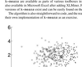
Let us ﬁrst show an example ofk-meanson an artiﬁcial dataset to illustrate how

k-meansworks. We will use artiﬁcial data drawn from four 2-D Gaussians and

use a value of k = 4; the dataset is illustrated in Figure 2.1. Data drawn from a

particular Gaussian is plotted in the same color in Figure 2.1. The blue data consists

of 200 points drawn from a Gaussian with mean at (−3,−3) and covariance

ma-trix.0625×I, where I is the identity matrix. The green data consists of 200 points

drawn from a Gaussian with mean at (3,−3) and covariance matrix I. Finally, we

have overlapping yellow and red data drawn from two nearby Gaussians. The yellow

data consists of 150 points drawn from a Gaussian with mean (−1,2) and covariance

matrix I, while the red data consists of 150 points drawn from a Gaussian with mean (1,2) and covariance matrix I. Despite the overlap between the red and yellow points,

one would expectk-meansto do well since we do have the right value of k and the

data is generated by a mixture of spherical Gaussians, thus matching nicely with the underlying assumptions of the algorithm.

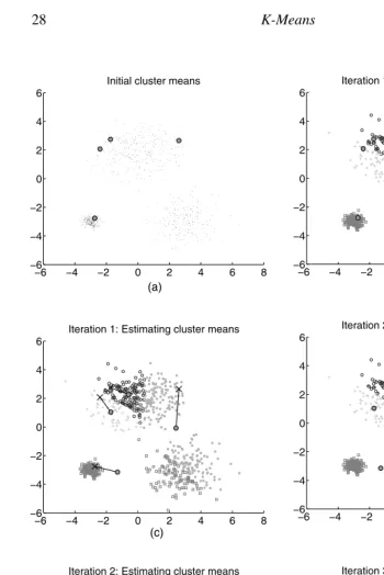
The ﬁrst step ink-meansis to initialize the cluster representatives. This is

illus-trated in Figure 2.2a, where k points in the dataset have been picked randomly. In this figure and the following figures, the cluster means C will be represented by a large colored circle with a black outline. The color corresponds to the cluster ID of that particular cluster, and all points assigned to that cluster are represented as points of the same color. These colors have no definite connection with the colors in Figure 2.1 (see Exercise 7). Since points have not been assigned cluster IDs in Figure 2.2a, they are plotted in black.

The next step is to assign all points to their closest cluster representative; this is illustrated in Figure 2.2b, where each point has been plotted to match the color of its

closest cluster representative. The third step ink-meansis to update the k cluster

representatives to correspond to the mean of all points currently assigned to that clus-ter. This step is illustrated in Figure 2.2c. In particular, we have plotted the old cluster representatives with a black “X” symbol and the new, updated cluster representatives as a large colored circle with a black outline. There is also a line connecting the old cluster mean with the new, updated cluster mean. One can observe that the cluster representatives have moved to reﬂect the current centroids of each cluster.

Thek-meansalgorithm now iterates between two steps until convergence: reas-signing points in D to their closest cluster representative and updating the k cluster

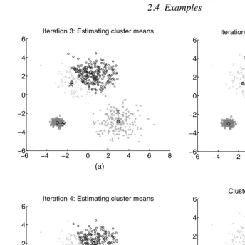
representatives. We have illustrated the ﬁrst four iterations ofk-meansin Figures

2.2 and 2.3. The ﬁnal clusters after convergence are shown in Figure 2.3d. Note that this example took eight iterations to converge. Visually, however, there is little change in the diagrams between iterations 4 and 8, and these pictures are omitted for space reasons. As one can see by comparing Figure 2.3d with Figure 2.1, the clusters found byk-meansmatch well with the true, underlying distribution.

In the previous section, we mentioned thatk-meansis sensitive to the initial points

(8)

−6 −4 −2 0 (a)

2 4 6 8

−6 −4 −2 0 2 4 6

Initial cluster means

−6 −4 −2 0

(b)

2 4 6 8

−6 −4 −2 0 2 4 6

Iteration 1: Assigning cluster IDs

−6 −4 −2 0

(c)

2 4 6 8

−6 −4 −2 0 2 4 6

Iteration 1: Estimating cluster means

−6 −4 −2 0 2 4 6 8

−6 −4 −2 0 2 4 6

(d)

−6 −4 −2 0 2 4 6 8

−6 −4 −2 0 2 4 6

(e)

−6 −4 −2 0 2 4 6 8

−6 −4 −2 0 2 4 6

[image:8.612.50.401.47.572.2]

(f)

(9)

2.4 Examples 29

−6 −4 −2 0 2 4 6 8

−6 −4 −2 0 2 4 6

(a)

−6 −4 −2 0 2 4 6 8

−6 −4 −2 0 2 4 6

(b)

−6 −4 −2 0 2 4 6 8

−6 −4 −2 0 2 4 6

(c)

−6 −4 −2 0

(d)

2 4 6 8

−6 −4 −2 0 2 4 6

[image:9.612.53.397.55.399.2]

Clusters after convergence

Figure 2.3 k-meanson artiﬁcial data. (Continued from Figure 2.2.)

initialized poorly on the same artiﬁcial dataset used in Figures 2.2 and 2.3. Figures 2.4a and c show two initializations that lead to poor clusters in Figures 2.4b and d. These results are considered poor since they do not correspond well to the true underlying distribution.

Finally, let us examine the performance ofk-meanson a simple, classic

bench-mark dataset. In our example, we use the Iris dataset (available from the UCI data mining repository), which contains 150 data points from three classes. Each class rep-resents a different species of the Iris ﬂower, and there are 50 points from each class. While there are four dimensions (representing sepal width, sepal length, petal width, and petal length), only two dimensions (petal width and petal length) are necessary to discriminate the three classes. The Iris dataset is plotted in Figure 2.5a along the dimensions of petal width and petal length.

In Figure 2.5b, we show an example of thek-meansalgorithm run on the Iris

(10)

−6 −4 −2 0 (a)

2 4 6 8

−6 −4 −2 0 2 4 6

−6 −4 −2 0 2 4 6 8

−6 −4 −2 0 2 4 6

(b)

−6 −4 −2 0 2 4 6 8

−6 −4 −2 0 2 4 6

(c)

−6 −4 −2 0 2 4 6 8

−6 −4 −2 0 2 4 6

[image:10.612.54.397.47.387.2]

(d)

Figure 2.4 Examples of poor clustering after poor initialization; these resultant clusters are considered “poor” in the sense that they do not match well with the true, underlying distribution.

k-meansalgorithm is able to cluster the data points such that each cluster is com-posed mostly of ﬂowers from the same species.

2.5 Advanced Topics

In this section, we discuss some generalizations, connections, and extensions that have

been made to thek-meansalgorithm. However, we should note that this section is

far from exhaustive. Research onk-meanshas been extensive and is still active.

Instead, the goal of this section is to complement some of the previously discussed

(11)

2.5 Advanced Topics 31

1 2 3 4 5 6 7

0 0.5 1 1.5 2 2.5

Petal Length

Petal Width

Iris Dataset

1 2 3 4 5 6 7

0 0.5 1 1.5 2 2.5

Petal Length

Petal Width

Iris dataset: clusters after convergence

[image:11.612.60.394.62.213.2]

(a) (b)

Figure 2.5 (a) Iris dataset; each color is a different species of Iris; (b) Result of k-means on Iris dataset; each color is a different cluster; note that there is not necessarily a correspondence between colors in (a) and (b) (see Exercise 7).

As mentioned earlier,k-meansis closely related to ﬁtting a mixture of k isotropic

Gaussians to the data. Moreover, the generalization of the distance measure to all Bregman divergences is related to ﬁtting the data with a mixture of k components from the exponential family of distributions. Another broad generalization is to view

the “means” as probabilistic models instead of points in Rd. Here, in the assignment

step, each data point is assigned to the model most likely to have generated it. In the “relocation” step, the model parameters are updated to best ﬁt the assigned datasets.

Such model-based k-means [23] allow one to cater to more complex data, for

example, sequences described by Hidden Markov models.

One can also “kernelize”k-means[5]. Though boundaries between clusters are

still linear in the implicit high-dimensional space, they can become nonlinear when

projected back to the original space, thus allowing kernelk-meansto deal with

more complex clusters. Dhillon et al. [5] have shown a close connection between

kernelk-meansand spectral clustering. The K-medoid [15] algorithm is similar to

k-means, except that the centroids have to belong to the dataset being clustered. Fuzzy c-means [6] is also similar, except that it computes fuzzy membership functions for each cluster rather than a hard one.

To deal with very large datasets, substantial effort has also gone into further

speed-ing upk-means, most notably by using kd-trees [19] or exploiting the triangular

inequality [7] to avoid comparing each data point with all the centroids during the assignment step.

Finally, we discuss two straightforward extensions of k-means. The ﬁrst is a

variant ofk-meanscalledsoft k-means. In the standardk-meansalgorithm,

each point xibelongs to one and only one cluster. Insoft k-means, this constraint

is relaxed, and each point xican belong to each cluster with some unknown probability.

(12)

that describe the likelihood that xibelongs to each cluster. These weights are based

on the distance of xi to each of the cluster representatives C, where the probability

that xiis from cluster j is proportional to the similarity between xiand cj. The cluster

representatives in this case are found by taking the expected value of the cluster mean over all points in the dataset D.

The second extension ofk-meansdeals with semisupervised learning. In the

intro-duction, we made a distinction between supervised learning and unsupervised learn-ing. In brief, supervised learning makes use of class labels while unsupervised learning

does not. Thek-meansalgorithm is a purely unsupervised algorithm. There also

exists a category of learning algorithms called semisupervised algorithms. Semisu-pervised learning algorithms are capable of making use of both labeled and unlabeled data. Semisupervised learning is a useful compromise between purely supervised methods and purely unsupervised methods. Supervised learning methods typically require very large amounts of labeled data; semisupervised methods are useful when very few labeled examples are available. Unsupervised learning methods, which do not look at class labels, may learn models inappropriate for the application at hand.

When runningk-means, one has no control over the ﬁnal clusters that are

discov-ered; these clusters may or may not correspond well to some underlying concept that one is interested in. For example, in Figure 2.5b, a poor initialization may have resulted in clusters which do not correspond well to the Iris species in the dataset. Semisupervised methods, which can take guidance in the form of labeled points, are more likely to create clusters which correspond to a given set of class labels.

Research into semisupervised variants ofk-meansinclude [22] and [2]. One of the

algorithms from [2] calledseeded k-meansis a simple extension tok-means

that uses labeled data to help initialize the value of k and the cluster representatives C. In this approach, k is chosen to be the same as the number of classes in the labeled

data, while cjis initialized as the mean of all labeled points in the j th class. Note that,

unlike unsupervisedk-means, there is now a known correspondence between the

j th cluster and the j th class. After initialization,seeded k-meansiterates over

the same two steps ask-means(updating cluster memberships and updating cluster

means) until convergence.

2.6 Summary

Thek-meansalgorithm is a simple iterative clustering algorithm that partitions a dataset into k clusters. At its core, the algorithm works by iterating over two steps: (1) clustering all points in the dataset based on the distance between each point and its closest cluster representative and (2) reestimating the cluster representatives.

Limita-tions of thek-meansalgorithm include the sensitivity ofk-meansto initialization

and determining the value of k.

Despite its drawbacks,k-meansremains the most widely used partitional

(13)

2.7 Exercises 33

reasonably scalable, and can be easily modiﬁed to deal with different scenarios such as semisupervised learning or streaming data. Continual improvements and general-izations of the basic algorithm have ensured its continued relevance and gradually increased its effectiveness as well.

2.7 Exercises

1. Using the standard benchmark Iris dataset (available online from the UCI

dataset repository), runk-meansto obtain results similar to Figure 2.5b. It is

sufﬁcient to look at only the attributes of “petal width” and “petal length.” What happens when one uses a value for k other than three? How do different cluster initializations affect the ﬁnal clusters? Why are these results potentially different than the results given in Figure 2.5b?

2. Prove that the value of thek-meansobjective function converges when

k-meansis run.

3. Describe three advantages and three disadvantages ofk-meanscompared to

other clustering methods (e.g., agglomerative clustering).

4. Describe or plot a two-dimensional example wherek-meanswould be

un-suitable for ﬁnding clusters.

5. Ink-means, after the cluster means have converged, what is the shape of the

cluster boundaries? How is this related to Voronoi tesselations?

6. Doesk-meansguarantee that points within the same cluster are more similar

than points from different clusters? That is, prove or disprove that, after

k-meanshas converged, the squared Euclidean distance between two points in the same cluster is always less than the squared Euclidean distance between two points from different clusters.

7. Assume one is given a hypothetical dataset D consisting of 10 points.k-means

is run twice on this dataset. Let us denote the cluster IDs of the 10 points in D

as a vector m, where mi, the i th entry in the vector, is the cluster ID of the i th

point in D.

The cluster IDs of the 10 points from the ﬁrst timek-meansis run are

m1=[1,1,1,2,2,2,3,3,3,3], while the cluster IDs obtained from the second

run ofk-meansare m2=[3,3,3,1,1,1,2,2,2,2].

What is the difference between the two sets of cluster IDs? Do the actual cluster IDs of the points in D mean anything? What does this imply when comparing the results of different clustering algorithms? What does this imply when comparing the results of clustering algorithms with known class labels?

8. Create your own implementation ofk-meansand a method of creating

artifi-cial data drawn from k Gaussian distributions. Test your code on the artifiartifi-cial

(14)

9. Using the code generated in the previous exercise, plot the average distance of each point from its cluster mean versus the number of clusters k. Is the average distance of a point from its cluster mean a good method of automatically determining the number of clusters k? Why or why not? What can potentially happen when the number of clusters k is equal to the number of points in the dataset?

10. Research and describe an extension to the standard k-means algorithm.

Depending on individual interests, this could include recent work on mak-ingk-meansmore computationally efﬁcient, work on extendingk-means to semisupervised learning, work on adapting other distance metrics into k-means, or many other possibilities.

References

[1] A. Banerjee, S. Merugu, I. Dhillon, and J. Ghosh. “Clustering with Bregman

divergences,” Journal of Machine Learning Research (JMLR), vol. 6, pp. 1705– 1749, 2005.

[2] S. Basu, A. Banerjee, and R. Mooney. “Semi-supervised clustering by seeding,”

International Conference on Machine Learning 2002, pp. 27–34, 2002.

[3] C. M. Bishop. Pattern Recognition and Machine Learning (Information Science

and Statistics). 2006.

[4] P. S. Bradley, K. P. Bennett, and A. Demiriz. “Constrained k-means clustering,”

Technical Report MSR-TR-2000-65, 2000.

[5] I. S. Dhillon, Y. Guan, and B. Kulis. “Kernel k-means: Spectral clustering and

normalized cuts,” KDD 2004, pp. 551–556, 2004.

[6] J. C. Dunn. “A fuzzy relative of the ISODATA process and its use in detecting

compact well-separated clusters,” Journal of Cybernetics, vol. 3, pp. 32–57, 1974.

[7] C. Elkan. “Using the triangle inequality to accelerate k-means,” International

Conference on Machine Learning 2003, pp. 147–153, 2003.

[8] C. Elkan. “Clustering with k-means: Faster, smarter, cheaper,” Keynote talk at

Workshop on Clustering High-Dimensional Data, SIAM International Confer-ence on Data Mining, 2004.

[9] E. Forgey. “Cluster analysis of multivariate data: Efﬁciency vs. interpretability

of classiﬁcation,” Biometrics, 21, pp. 768, 1965.

[10] H. P. Friedman and J. Rubin. “On some invariant criteria for grouping data,”

(15)

References 35

[11] R. M. Gray and D. L. Neuhoff. “Quantization,” IEEE Transactions on

Infor-mation Theory, vol. 44, no. 6, pp. 2325–2384, 1998.

[12] G. Hamerly and C. Elkan. “Learning the k in k-means,” Neural Information

Processing Systems, 2003.

[13] A. K. Jain and R. C. Dubes. Algorithms for Clustering Data, Prentice Hall,

1988.

[14] T. Kanungo, D. M. Mount, N. Netanyahu, C. Piatko, R. Silverman, and A. Y.

Wu. “A local search approximation algorithm for k-means clustering,” Com-putational Geometry: Theory and Applications, 28 (2004), pp. 89–112, 2004.

[15] L. Kaufman and P. J. Rousseeuw. Finding Groups in Data: An Introduction to

Cluster Analysis, 1990.

[16] S. P. Lloyd. “Least squares quantization in PCM,” unpublished Bell Lab. Tech.

Note, portions presented at the Institute of Mathematical Statistics Meet., Atlantic City, NJ, Sept. 1957. Also, IEEE Trans. Inform. Theory (Special Issue on Quantization), vol. IT-28, pp. 129–137, Mar. 1982.

[17] J. McQueen. “Some methods for classiﬁcation and analysis of mutivariate

observations,” Proc. 5th Berkeley Symp. Math., Statistics and Probability, 1, pp. 281–296, 1967.

[18] G. W. Milligan. “Clustering validation: Results and implications for applied

analyses,” Clustering and Classiﬁcation, P. Arabie, L. J. Hubery, and G. De Soete, ed., pp. 341–375, 1996.

[19] D. Pelleg and A. Moore. “Accelerating exact k-means algorithms with

geomet-ric reasoning,” KDD 1999, pp. 227–281, 1999.

[20] D. Pelleg and A. Moore. “X-means: Extending k-means with efﬁcient

estima-tion of the number of clusters,” Internaestima-tional Conference on Machine Learning 2000, pp. 727–734, 2000.

[21] M. Steinbach, G. Karypis, and V. Kumar. “A comparison of document clustering

techniques,” Proc. KDD Workshop on Text Mining, 2000.

[22] K. Wagstaff, C. Cardie, S. Rogers, S. Schr¨odl. “Constrained k-means clustering

with background knowledge,” International Conference on Machine Learning 2001, pp. 577–584, 2001.

[23] S. Zhong and J. Ghosh. “A uniﬁed framework for model-based clustering,”