Python for Finance
Yves Hilpisch
Preface
Not too long ago, Python as a programming language and platform technology was
considered exotic — if not completely irrelevant — in the financial industry. By contrast, in 2014 there are many examples of large financial institutions — like Bank of America Merrill Lynch with its Quartz project, or JP Morgan Chase with the Athena project — that strategically use Python alongside other established technologies to build, enhance, and
maintain some of their core IT systems. There is also a multitude of larger and smaller hedge funds that make heavy use of Python’s capabilities when it comes to efficient
financial application development and productive financial analytics efforts.
Similarly, many of today’s Master of Financial Engineering programs (or programs awarding similar degrees) use Python as one of the core languages for teaching the
translation of quantitative finance theory into executable computer code. Educational programs and trainings targeted to finance professionals are also increasingly
incorporating Python into their curricula. Some now teach it as the main implementation
language.
There are many reasons why Python has had such recent success and why it seems it will
continue to do so in the future. Among these reasons are its syntax, the ecosystem of scientific and data analytics libraries available to developers using Python, its ease of integration with almost any other technology, and its status as open source. (See Chapter 1 for a few more insights in this regard.)
For that reason, there is an abundance of good books available that teach Python from
different angles and with different focuses. This book is one of the first to introduce and teach Python for finance — in particular, for quantitative finance and for financial
analytics. The approach is a practical one, in that implementation and illustration come before theoretical details, and the big picture is generally more focused on than the most arcane parameterization options of a certain class or function.
Most of this book has been written in the powerful, interactive, browser-based IPython Notebook environment (explained in more detail in Chapter 2). This makes it possible to
provide the reader with executable, interactive versions of almost all examples used in this book.
Those who want to immediately get started with a full-fledged, interactive financial analytics environment for Python (and, for instance, R and Julia) should go to
http://oreilly.quant-platform.com and try out the Python Quant Platform (in combination with the IPython Notebook files and code that come with this book). You should also
have a look at DX analytics, a Python-based financial analytics library. My other book,
Derivatives Analytics with Python (Wiley Finance), presents more details on the theory and numerical methods for advanced derivatives analytics. It also provides a wealth of readily usable Python code. Further material, and, in particular, slide decks and videos of
talks about Python for Quant Finance can be found on my private website.
If you want to get involved in Python for Quant Finance community events, there are
Finance-London/) and New York City (cf. http://www.meetup.com/Python-for-Quant-Finance-NYC/). There are also For Python Quants conferences and workshops several times a year (cf. http://forpythonquants.com and http://pythonquants.com).
I am really excited that Python has established itself as an important technology in the
Conventions Used in This Book
The following typographical conventions are used in this book:
Italic
Indicates new terms, URLs, and email addresses.
Constant width
Used for program listings, as well as within paragraphs to refer to software packages, programming languages, file extensions, filenames, program elements such as
variable or function names, databases, data types, environment variables, statements, and keywords.
Constant width italic
Shows text that should be replaced with user-supplied values or by values determined by context.
TIP
This element signifies a tip or suggestion.
WARNING
Using Code Examples
Supplemental material (in particular, IPython Notebooks and Python scripts/modules) is available for download at http://oreilly.quant-platform.com.
This book is here to help you get your job done. In general, if example code is offered with this book, you may use it in your programs and documentation. You do not need to contact us for permission unless you’re reproducing a significant portion of the code. For example, writing a program that uses several chunks of code from this book does not require permission. Selling or distributing a CD-ROM of examples from O’Reilly books does require permission. Answering a question by citing this book and quoting example code does not require permission. Incorporating a significant amount of example code from this book into your product’s documentation does require permission.
We appreciate, but do not require, attribution. An attribution usually includes the title, author, publisher, and ISBN. For example: “Python for Finance by Yves Hilpisch (O’Reilly). Copyright 2015 Yves Hilpisch, 978-1-491-94528-5.”
Safari® Books Online
NOTE
Safari Books Online is an on-demand digital library that delivers expert content in both book and video form from the world’s leading authors in technology and business.
Technology professionals, software developers, web designers, and business and creative professionals use Safari Books Online as their primary resource for research, problem solving, learning, and certification training.
Safari Books Online offers a range of plans and pricing for enterprise, government, education, and individuals.
Members have access to thousands of books, training videos, and prepublication manuscripts in one fully searchable database from publishers like O’Reilly Media, Prentice Hall Professional, Addison-Wesley Professional, Microsoft Press, Sams, Que, Peachpit Press, Focal Press, Cisco Press, John Wiley & Sons, Syngress, Morgan
Kaufmann, IBM Redbooks, Packt, Adobe Press, FT Press, Apress, Manning, New Riders, McGraw-Hill, Jones & Bartlett, Course Technology, and hundreds more. For more
How to Contact Us
Please address comments and questions concerning this book to the publisher:
O’Reilly Media, Inc.
1005 Gravenstein Highway North Sebastopol, CA 95472
800-998-9938 (in the United States or Canada) 707-829-0515 (international or local)
707-829-0104 (fax)
We have a web page for this book, where we list errata, examples, and any additional information. You can access this page at http://bit.ly/python-finance.
To comment or ask technical questions about this book, send email to [email protected].
For more information about our books, courses, conferences, and news, see our website at http://www.oreilly.com.
Find us on Facebook: http://facebook.com/oreilly
Follow us on Twitter: http://twitter.com/oreillymedia
Acknowledgments
I want to thank all those who helped to make this book a reality, in particular those who have provided honest feedback or even completely worked out examples, like Ben Lerner, James Powell, Michael Schwed, Thomas Wiecki or Felix Zumstein. Similarly, I would like to thank reviewers Hugh Brown, Jennifer Pierce, Kevin Sheppard, and Galen
Wilkerson. The book benefited from their valuable feedback and the many suggestions.
The book has also benefited significantly as a result of feedback I received from the participants of the many conferences and workshops I was able to present at in 2013 and 2014: PyData, For Python Quants, Big Data in Quant Finance, EuroPython, EuroScipy, PyCon DE, PyCon Ireland, Parallel Data Analysis, Budapest BI Forum and CodeJam. I also got valuable feedback during my many presentations at Python meetups in Berlin,
London, and New York City.
Last but not least, I want to thank my family, which fully accepts that I do what I love doing most and this, in general, rather intensively. Writing and finishing a book of this length over the course of a year requires a large time commitment — on top of my usually heavy workload and packed travel schedule — and makes it necessary to sit sometimes more hours in solitude in front the computer than expected. Therefore, thank you Sandra, Lilli, and Henry for your understanding and support. I dedicate this book to my lovely wife Sandra, who is the heart of our family.
Part I. Python and Finance
This part introduces Python for finance. It consists of three chapters:
Chapter 1 briefly discusses Python in general and argues why Python is indeed well
suited to address the technological challenges in the finance industry and in financial (data) analytics.
Chapter 2, on Python infrastructure and tools, is meant to provide a concise overview
of the most important things you have to know to get started with interactive analytics and application development in Python; the related Appendix A surveys
some selected best practices for Python development.
Chapter 3 immediately dives into three specific financial examples; it illustrates how to calculate implied volatilities of options with Python, how to simulate a financial
model with Python and the array library NumPy, and how to implement a backtesting
for a trend-based investment strategy. This chapter should give the reader a feeling for what it means to use Python for financial analytics — details are not that
Chapter 1. Why Python for Finance?
Banks are essentially technology firms.
What Is Python?
Python is a high-level, multipurpose programming language that is used in a wide range of
domains and technical fields. On the Python website you find the following executive
summary (cf. https://www.python.org/doc/essays/blurb):
Python is an interpreted, object-oriented, level programming language with dynamic semantics. Its high-level built in data structures, combined with dynamic typing and dynamic binding, make it very attractive for Rapid Application Development, as well as for use as a scripting or glue language to connect existing components together. Python’s simple, easy to learn syntax emphasizes readability and therefore reduces the cost of program maintenance. Python supports modules and packages, which encourages program modularity and code reuse. The Python interpreter and the extensive standard library are available in source or binary form without charge for all major platforms, and can be freely distributed.
This pretty well describes whyPython has evolved into one of the major programming
languages as of today. Nowadays, Python is used by the beginner programmer as well as
by the highly skilled expert developer, at schools, in universities, at web companies, in large corporations and financial institutions, as well as in any scientific field.
Among others, Python is characterized by the following features:
Open source
Python and the majority of supporting libraries and tools available are open source
and generally come with quite flexible and open licenses.
Interpreted
The reference CPython implementation is an interpreter of the language that
translates Python code at runtime to executable byte code.
Multiparadigm
Python supports different programming and implementation paradigms, such as
object orientation and imperative, functional, or procedural programming.
Multipurpose
Python can be used for rapid, interactive code development as well as for building
large applications; it can be used for low-level systems operations as well as for high-level analytics tasks.
Cross-platform
Python is available for the most important operating systems, such as Windows, Linux, and Mac OS; it is used to build desktop as well as web applications; it can be
used on the largest clusters and most powerful servers as well as on such small devices as the Raspberry Pi (cf. http://www.raspberrypi.org).
Dynamically typed
Types in Python are in general inferred during runtime and not statically declared as
in most compiled languages.
Indentation aware
for marking code blocks instead of parentheses, brackets, or semicolons.
Garbage collecting
Python has automated garbage collection, avoiding the need for the programmer to
manage memory.
When it comes to Python syntax and what Python is all about, Python Enhancement
Proposal 20 — i.e., the so-called “Zen of Python” — provides the major guidelines. It can be accessed from every interactive shell with the command import this:
$ ipython
Python 2.7.6 |Anaconda 1.9.1 (x86_64)| (default, Jan 10 2014, 11:23:15) Type “copyright”, “credits” or “license” for more information.
IPython 2.0.0—An enhanced Interactive Python.
? -> Introduction and overview of IPython’s features. %quickref -> Quick reference.
help -> Python’s own help system.
object? -> Details about ‘object’, use ‘object??’ for extra details.
In [1]: import this
The Zen of Python, by Tim Peters
Beautiful is better than ugly. Explicit is better than implicit. Simple is better than complex. Complex is better than complicated. Flat is better than nested.
Sparse is better than dense. Readability counts.
Special cases aren’t special enough to break the rules. Although practicality beats purity.
Errors should never pass silently. Unless explicitly silenced.
In the face of ambiguity, refuse the temptation to guess.
There should be one—and preferably only one—obvious way to do it. Although that way may not be obvious at first unless you’re Dutch. Now is better than never.
Although never is often better than *right* now.
If the implementation is hard to explain, it’s a bad idea. If the implementation is easy to explain, it may be a good idea. Namespaces are one honking great idea—let’s do more of those!
Brief History of Python
Although Python might still have the appeal of something new to some people, it has been
around for quite a long time. In fact, development efforts began in the 1980s by Guido van Rossum from the Netherlands. He is still active in Python development and has been
awarded the title of Benevolent Dictator for Life by the Python community (cf.
http://en.wikipedia.org/wiki/History_of_Python). The following can be considered milestones in the development of Python:
Python 0.9.0 released in 1991 (first release) Python 1.0 released in 1994
It is remarkable, and sometimes confusing to Python newcomers, that there are two major
versions available, still being developed and, more importantly, in parallel use since 2008. As of this writing, this will keep on for quite a while since neither is there 100% code compatibility between the versions, nor are all popular libraries available for Python 3.x.
The majority of code available and in production is still Python 2.6/2.7, and this book is
based on the 2.7.x version, although the majority of code examples should work with
versions 3.x as well.
The Python Ecosystem
A major feature of Python as an ecosystem, compared to just being a programming
language, is the availability of a large number of libraries and tools. These libraries and tools generally have to be imported when needed (e.g., a plotting library) or have to be started as a separate system process (e.g., a Python development environment). Importing
means making a library available to the current namespace and the current Python
interpreter process.
Python itself already comes with a large set of libraries that enhance the basic interpreter
in different directions. For example, basic mathematical calculations can be done without any importing, while more complex mathematical functions need to be imported through the math library:
In [2]: 100 * 2.5 + 50 Out[2]: 300.0
In [3]: log(1) …
NameError: name ‘log’ is not defined
In [4]: from math import *
In [5]: log(1) Out[5]: 0.0
Although the so-called “star import” (i.e., the practice of importing everything from a library via from library import *) is sometimes convenient, one should generally use
an alternative approach that avoids ambiguity with regard to name spaces and relationships of functions to libraries. This then takes on the form:
In [6]: import math
In [7]: math.log(1) Out[7]: 0.0
While math is a standard Python library available with any installation, there are many
more libraries that can be installed optionally and that can be used in the very same
fashion as the standard libraries. Such libraries are available from different (web) sources. However, it is generally advisable to use a Python distribution that makes sure that all
libraries are consistent with each other (see Chapter 2 for more on this topic).
The code examples presented so far all use IPython (cf. http://www.ipython.org), which is
probably the most popular interactive development environment (IDE) for Python.
Although it started out as an enhanced shell only, it today has many features typically found in IDEs (e.g., support for profiling and debugging). Those features missing are typically provided by advanced text/code editors, like Sublime Text (cf.
text/code editor of choice to form the basic tool set for a Python development process.
IPython is also sometimes called the killer application of the Python ecosystem. It
enhances the standard interactive shell in many ways. For example, it provides improved command-line history functions and allows for easy object inspection. For instance, the help text for a function is printed by just adding a ? behind the function name (adding ??
will provide even more information):
In [8]: math.log?
Type: builtin_function_or_method String Form:<built-in function log> Docstring:
log(x[, base])
Return the logarithm of x to the given base.
If the base not specified, returns the natural logarithm (base e) of x.
In [9]:
IPython comes in three different versions: a shell version, one based on a QT graphical
user interface (the QT console), and a browser-based version (the Notebook). This is just
meant as a teaser; there is no need to worry about the details now since Chapter 2 introduces IPython in more detail.
Python User Spectrum
Python does not only appeal to professional software developers; it is also of use for the
casual developer as well as for domain experts and scientific developers.
Professional software developers find all that they need to efficiently build large applications. Almost all programming paradigms are supported; there are powerful development tools available; and any task can, in principle, be addressed with Python.
These types of users typically build their own frameworks and classes, also work on the fundamental Python and scientific stack, and strive to make the most of the ecosystem.
Scientific developers or domain experts are generally heavy users of certain libraries and frameworks, have built their own applications that they enhance and optimize over time, and tailor the ecosystem to their specific needs. These groups of users also generally engage in longer interactive sessions, rapidly prototyping new code as well as exploring and visualizing their research and/or domain data sets.
Casual programmers like to use Python generally for specific problems they know that Python has its strengths in. For example, visiting the gallery page of matplotlib, copying
a certain piece of visualization code provided there, and adjusting the code to their specific needs might be a beneficial use case for members of this group.
There is also another important group of Python users: beginner programmers, i.e., those
that are just starting to program. Nowadays, Python has become a very popular language
at universities, colleges, and even schools to introduce students to programming.[1] A major reason for this is that its basic syntax is easy to learn and easy to understand, even for the nondeveloper. In addition, it is helpful that Python supports almost all
programming styles.[2]
The Scientific Stack
comprises, among others, the following libraries:
NumPy
NumPy provides a multidimensional array object to store homogenous or
heterogeneous data; it also provides optimized functions/methods to operate on this array object.
SciPy
SciPy is a collection of sublibraries and functions implementing important standard
functionality often needed in science or finance; for example, you will find functions for cubic splines interpolation as well as for numerical integration.
matplotlib
This is the most popular plotting and visualization library for Python, providing both
2D and 3D visualization capabilities.
PyTables
PyTables is a popular wrapper for the HDF5 data storage library (cf.
http://www.hdfgroup.org/HDF5/); it is a library to implement optimized, disk-based I/O operations based on a hierarchical database/file format.
pandas
pandas builds on NumPy and provides richer classes for the management and analysis
of time series and tabular data; it is tightly integrated with matplotlib for plotting
and PyTables for data storage and retrieval.
Depending on the specific domain or problem, this stack is enlarged by additional
libraries, which more often than not have in common that they build on top of one or more of these fundamental libraries. However, the least common denominator or basic building block in general is the NumPyndarray class (cf. Chapter 4).
Taking Python as a programming language alone, there are a number of other languages
available that can probably keep up with its syntax and elegance. For example, Ruby is
quite a popular language often compared to Python. On the language’s website you find
the following description:
A dynamic, open source programming language with a focus on simplicity and productivity. It has an elegant syntax that is natural to read and easy to write.
The majority of people using Python would probably also agree with the exact same
statement being made about Python itself. However, what distinguishes Python for many
users from equally appealing languages like Ruby is the availability of the scientific stack.
This makes Python not only a good and elegant language to use, but also one that is
capable of replacing domain-specific languages and tool sets like Matlab or R. In addition,
Technology in Finance
Now that we have some rough ideas of what Python is all about, it makes sense to step
back a bit and to briefly contemplate the role of technology in finance. This will put us in a position to better judge the role Python already plays and, even more importantly, will
probably play in the financial industry of the future.
In a sense, technology per se is nothing special to financial institutions (as compared, for instance, to industrial companies) or to the finance function (as compared to other
corporate functions, like logistics). However, in recent years, spurred by innovation and also regulation, banks and other financial institutions like hedge funds have evolved more and more into technology companies instead of being just financial intermediaries.
Technology has become a major asset for almost any financial institution around the globe, having the potential to lead to competitive advantages as well as disadvantages. Some background information can shed light on the reasons for this development.
Technology Spending
Banks and financial institutions together form the industry that spends the most on technology on an annual basis. The following statement therefore shows not only that technology is important for the financial industry, but that the financial industry is also really important to the technology sector:
Banks will spend 4.2% more on technology in 2014 than they did in 2013, according to IDC analysts. Overall IT spend in financial services globally will exceed $430 billion in 2014 and surpass $500 billion by 2020, the analysts say.
— Crosman 2013
Large, multinational banks today generally employ thousands of developers that maintain existing systems and build new ones. Large investment banks with heavy technological requirements show technology budgets often of several billion USD per year.
Technology as Enabler
The technological development has also contributed to innovations and efficiency improvements in the financial sector:
Technological innovations have contributed significantly to greater efficiency in the derivatives market. Through innovations in trading technology, trades at Eurex are today executed much faster than ten years ago despite the strong increase in trading volume and the number of quotes … These strong improvements have only been possible due to the constant, high IT investments by derivatives exchanges and clearing houses.
— Deutsche Börse Group 2008
As a side effect of the increasing efficiency, competitive advantages must often be looked for in ever more complex products or transactions. This in turn inherently increases risks and makes risk management as well as oversight and regulation more and more difficult. The financial crisis of 2007 and 2008 tells the story of potential dangers resulting from such developments. In a similar vein, “algorithms and computers gone wild” also
represent a potential risk to the financial markets; this materialized dramatically in the so-called flash crash of May 2010, where automated selling led to large intraday drops in certain stocks and stock indices (cf. http://en.wikipedia.org/wiki/2010_Flash_Crash).
On the one hand, technology advances reduce cost over time, ceteris paribus. On the other hand, financial institutions continue to invest heavily in technology to both gain market share and defend their current positions. To be active in certain areas in finance today often brings with it the need for large-scale investments in both technology and skilled staff. As an example, consider the derivatives analytics space (see also the case study in Part III of the book):
Aggregated over the total software lifecycle, firms adopting in-house strategies for OTC [derivatives] pricing will require investments between $25 million and $36 million alone to build, maintain, and enhance a complete derivatives library.
— Ding 2010
Not only is it costly and time-consuming to build a full-fledged derivatives analytics library, but you also need to have enough experts to do so. And these experts have to have the right tools and technologies available to accomplish their tasks.
Another quote about the early days of Long-Term Capital Management (LTCM), formerly one of the most respected quantitative hedge funds — which, however, went bust in the late 1990s — further supports this insight about technology and talent:
Meriwether spent $20 million on a state-of-the-art computer system and hired a crack team of financial engineers to run the show at LTCM, which set up shop in Greenwich, Connecticut. It was risk management on an industrial level.
— Patterson 2010
The same computing power that Meriwether had to buy for millions of dollars is today probably available for thousands. On the other hand, trading, pricing, and risk
management have become so complex for larger financial institutions that today they need to deploy IT infrastructures with tens of thousands of computing cores.
Ever-Increasing Speeds, Frequencies, Data Volumes
There is one dimension of the finance industry that has been influenced most by
technological advances: the speed and frequency with which financial transactions are decided and executed. The recent book by Lewis (2014) describes so-called flash trading
— i.e., trading at the highest speeds possible — in vivid detail.
On the one hand, increasing data availability on ever-smaller scales makes it necessary to react in real time. On the other hand, the increasing speed and frequency of trading let the data volumes further increase. This leads to processes that reinforce each other and push the average time scale for financial transactions systematically down:
Renaissance’s Medallion fund gained an astonishing 80 percent in 2008, capitalizing on the market’s extreme volatility with its lightning-fast computers. Jim Simons was the hedge fund world’s top earner for the year, pocketing a cool $2.5 billion.
— Patterson 2010
Thirty years’ worth of daily stock price data for a single stock represents roughly 7,500 quotes. This kind of data is what most of today’s finance theory is based on. For example, theories like the modern portfolio theory (MPT), the capital asset pricing model (CAPM), and value-at-risk (VaR) all have their foundations in daily stock price data.
time span of 30 years. This brings with it a number of challenges:
Data processing
It does not suffice to consider and process end-of-day quotes for stocks or other financial instruments; “too much” happens during the day for some instruments during 24 hours for 7 days a week.
Analytics speed
Decisions often have to be made in milliseconds or even faster, making it necessary to build the respective analytics capabilities and to analyze large amounts of data in real time.
Theoretical foundations
Although traditional finance theories and concepts are far from being perfect, they have been well tested (and sometimes well rejected) over time; for the millisecond scales important as of today, consistent concepts and theories that have proven to be somewhat robust over time are still missing.
All these challenges can in principle only be addressed by modern technology. Something that might also be a little bit surprising is that the lack of consistent theories often is
addressed by technological approaches, in that high-speed algorithms exploit market microstructure elements (e.g., order flow, bid-ask spreads) rather than relying on some kind of financial reasoning.
The Rise of Real-Time Analytics
There is one discipline that has seen a strong increase in importance in the finance industry: financial and data analytics. This phenomenon has a close relationship to the insight that speeds, frequencies, and data volumes increase at a rapid pace in the industry. In fact, real-time analytics can be considered the industry’s answer to this trend.
Roughly speaking, “financial and data analytics” refers to the discipline of applying
software and technology in combination with (possibly advanced) algorithms and methods to gather, process, and analyze data in order to gain insights, to make decisions, or to
fulfill regulatory requirements, for instance. Examples might include the estimation of sales impacts induced by a change in the pricing structure for a financial product in the retail branch of a bank. Another example might be the large-scale overnight calculation of credit value adjustments (CVA) for complex portfolios of derivatives trades of an
investment bank.
There are two major challenges that financial institutions face in this context:
Big data
Banks and other financial institutions had to deal with massive amounts of data even before the term “big data” was coined; however, the amount of data that has to be processed during single analytics tasks has increased tremendously over time, demanding both increased computing power and ever-larger memory and storage capacities.
In the past, decision makers could rely on structured, regular planning, decision, and (risk) management processes, whereas they today face the need to take care of these functions in real time; several tasks that have been taken care of in the past via overnight batch runs in the back office have now been moved to the front office and are executed in real time.
Again, one can observe an interplay between advances in technology and
financial/business practice. On the one hand, there is the need to constantly improve analytics approaches in terms of speed and capability by applying modern technologies. On the other hand, advances on the technology side allow new analytics approaches that were considered impossible (or infeasible due to budget constraints) a couple of years or even months ago.
One major trend in the analytics space has been the utilization of parallel architectures on the CPU (central processing unit) side and massively parallel architectures on the GPGPU (general-purpose graphical processing units) side. Current GPGPUs often have more than 1,000 computing cores, making necessary a sometimes radical rethinking of what
Python for Finance
The previous section describes some selected aspects characterizing the role of technology in finance:
Costs for technology in the finance industry
Technology as an enabler for new business and innovation
Technology and talent as barriers to entry in the finance industry Increasing speeds, frequencies, and data volumes
The rise of real-time analytics
In this section, we want to analyze how Python can help in addressing several of the
challenges implied by these aspects. But first, on a more fundamental level, let us examine
Python for finance from a language and syntax standpoint.
Finance and Python Syntax
Most people who make their first steps with Python in a finance context may attack an
algorithmic problem. This is similar to a scientist who, for example, wants to solve a
differential equation, wants to evaluate an integral, or simply wants to visualize some data. In general, at this stage, there is only little thought spent on topics like a formal
development process, testing, documentation, or deployment. However, this especially seems to be the stage when people fall in love with Python. A major reason for this might
be that the Python syntax is generally quite close to the mathematical syntax used to
describe scientific problems or financial algorithms.
We can illustrate this phenomenon by a simple financial algorithm, namely the valuation of a European call option by Monte Carlo simulation. We will consider a Black-Scholes-Merton (BSM) setup (see also Chapter 3) in which the option’s underlying risk factor follows a geometric Brownian motion.
Suppose we have the following numerical parameter values for the valuation:
Initial stock index level S0 = 100
Strike price of the European call option K = 105 Time-to-maturity T = 1 year
Constant, riskless short rate r = 5% Constant volatility = 20%
In the BSM model, the index level at maturity is a random variable, given by Equation 1-1 with z being a standard normally distributed random variable.
The following is an algorithmic description of the Monte Carlo valuation procedure:
1. Draw I (pseudo)random numbers z(i), i ∈ {1, 2, …, I}, from the standard normal distribution.
2. Calculate all resulting index levels at maturity ST(i) for given z(i) and Equation 1-1. 3. Calculate all inner values of the option at maturity as hT(i) = max(ST(i) – K,0).
4. Estimate the option present value via the Monte Carlo estimator given in Equation 1-2.
Equation 1-2. Monte Carlo estimator for European option
We are now going to translate this problem and algorithm into Python code. The reader
might follow the single steps by using, for example, IPython — this is, however, not
really necessary at this stage.
First, let us start with the parameter values. This is really easy:
S0 = 100.
K = 105.
T = 1.0
r = 0.05
sigma = 0.2
Next, the valuation algorithm. Here, we will for the first time use NumPy, which makes life
quite easy for our second task:
from numpy import *
I = 100000
z = random.standard_normal(I)
ST = S0 * exp((r - 0.5 * sigma ** 2) * T + sigma * sqrt(T) * z)
hT = maximum(ST - K, 0)
C0 = exp(-r * T) * sum(hT) / I Third, we print the result:
print “Value of the European Call Option %5.3f” % C0 The output might be:[4]
Value of the European Call Option 8.019
Three aspects are worth highlighting:
Syntax
The Python syntax is indeed quite close to the mathematical syntax, e.g., when it
comes to the parameter value assignments.
Translation
single line of Python code.
Vectorization
One of the strengths of NumPy is the compact, vectorized syntax, e.g., allowing for
100,000 calculations within a single line of code.
This code can be used in an interactive environment like IPython. However, code that is
meant to be reused regularly typically gets organized in so-called modules (or scripts), which are single Python (i.e., text) files with the suffix .py. Such a module could in this
case look like Example 1-1 and could be saved as a file named bsm_mcs_euro.py.
Example 1-1. Monte Carlo valuation of European call option
#
# Monte Carlo valuation of European call option # in Black-Scholes-Merton model
# bsm_mcs_euro.py #
import numpy as np
# Parameter Values
S0 = 100. # initial index level
K = 105. # strike price
T = 1.0 # time-to-maturity
r = 0.05 # riskless short rate
sigma = 0.2 # volatility
I = 100000 # number of simulations
# Valuation Algorithm
z = np.random.standard_normal(I) # pseudorandom numbers
ST = S0 * np.exp((r - 0.5 * sigma ** 2) * T + sigma * np.sqrt(T) * z) # index values at maturity
hT = np.maximum(ST - K, 0) # inner values at maturity
C0 = np.exp(-r * T) * np.sum(hT) / I # Monte Carlo estimator
# Result Output
print “Value of the European Call Option %5.3f” % C0
The rather simple algorithmic example in this subsection illustrates that Python, with its
very syntax, is well suited to complement the classic duo of scientific languages, English and Mathematics. It seems that adding Python to the set of scientific languages makes it
more well rounded. We have
English for writing, talking about scientific and financial problems, etc.
Mathematics for concisely and exactly describing and modeling abstract aspects, algorithms, complex quantities, etc.
Python for technically modeling and implementing abstract aspects, algorithms, complex quantities, etc.
MATHEMATICS AND PYTHON SYNTAX
There is hardly any programming language that comes as close to mathematical syntax as Python. Numerical
algorithms are therefore simple to translate from the mathematical representation into the Pythonic
implementation. This makes prototyping, development, and code maintenance in such areas quite efficient with
Python.
representation and already quite close to the technical implementation. In addition to the algorithm itself, pseudocode takes into account how computers work in principle.
This practice generally has its cause in the fact that with most programming languages the technical implementation is quite “far away” from its formal, mathematical representation. The majority of programming languages make it necessary to include so many elements that are only technically required that it is hard to see the equivalence between the
mathematics and the code.
Nowadays, Python is often used in a pseudocode way since its syntax is almost analogous
to the mathematics and since the technical “overhead” is kept to a minimum. This is accomplished by a number of high-level concepts embodied in the language that not only have their advantages but also come in general with risks and/or other costs. However, it is safe to say that with Python you can, whenever the need arises, follow the same strict
implementation and coding practices that other languages might require from the outset. In that sense, Python can provide the best of both worlds: high-level abstraction and rigorous
implementation.
Efficiency and Productivity Through Python
At a high level, benefits from using Python can be measured in three dimensions:
Efficiency
How can Python help in getting results faster, in saving costs, and in saving time?
Productivity
How can Python help in getting more done with the same resources (people, assets,
etc.)?
Quality
What does Python allow us to do that we could not do with alternative technologies?
A discussion of these aspects can by nature not be exhaustive. However, it can highlight some arguments as a starting point.
Shorter time-to-results
A field where the efficiency of Python becomes quite obvious is interactive data analytics.
This is a field that benefits strongly from such powerful tools as IPython and libraries like pandas.
Consider a finance student, writing her master’s thesis and interested in Google stock prices. She wants to analyze historical stock price information for, say, five years to see how the volatility of the stock price has fluctuated over time. She wants to find evidence that volatility, in contrast to some typical model assumptions, fluctuates over time and is far from being constant. The results should also be visualized. She mainly has to do the following:
Download Google stock price data from the Web.
Plot the stock price data and the results.
These tasks are complex enough that not too long ago one would have considered them to be something for professional financial analysts. Today, even the finance student can easily cope with such problems. Let us see how exactly this works — without worrying about syntax details at this stage (everything is explained in detail in subsequent chapters).
First, make sure to have available all necessary libraries:
In [1]: import numpy as np
import pandas as pd
import pandas.io.data as web
Second, retrieve the data from, say, Google itself:
In [2]: goog = web.DataReader(‘GOOG’, data_source=‘google’, start=‘3/14/2009’, end=‘4/14/2014’) goog.tail()
Out[2]: Open High Low Close Volume Date
2014-04-08 542.60 555.00 541.61 554.90 3152406 2014-04-09 559.62 565.37 552.95 564.14 3324742 2014-04-10 565.00 565.00 539.90 540.95 4027743 2014-04-11 532.55 540.00 526.53 530.60 3916171 2014-04-14 538.25 544.10 529.56 532.52 2568020
5 rows × 5 columns
Third, implement the necessary analytics for the volatilities:
In [3]: goog[‘Log_Ret’] = np.log(goog[‘Close’] / goog[‘Close’].shift(1)) goog[‘Volatility’] = pd.rolling_std(goog[‘Log_Ret’],
window=252) * np.sqrt(252)
Fourth, plot the results. To generate an inline plot, we use the IPython magic command %matplotlib with the option inline:
In [4]: %matplotlib inline
goog[[‘Close’, ‘Volatility’]].plot(subplots=True, color=‘blue’, figsize=(8, 6))
Figure 1-1 shows the graphical result of this brief interactive session with IPython. It can
be considered almost amazing that four lines of code suffice to implement three rather complex tasks typically encountered in financial analytics: data gathering, complex and repeated mathematical calculations, and visualization of results. This example illustrates that pandas makes working with whole time series almost as simple as doing
Figure 1-1. Google closing prices and yearly volatility
Translated to a professional finance context, the example implies that financial analysts can — when applying the right Python tools and libraries, providing high-level abstraction
— focus on their very domain and not on the technical intrinsicalities. Analysts can react faster, providing valuable insights almost in real time and making sure they are one step ahead of the competition. This example of increased efficiency can easily translate into measurable bottom-line effects.
Ensuring high performance
In general, it is accepted that Python has a rather concise syntax and that it is relatively
efficient to code with. However, due to the very nature of Python being an interpreted
language, the prejudice persists that Python generally is too slow for compute-intensive
tasks in finance. Indeed, depending on the specific implementation approach, Python can
be really slow. But it does not have to be slow — it can be highly performing in almost any application area. In principle, one can distinguish at least three different strategies for better performance:
Paradigm
In general, many different ways can lead to the same result in Python, but with rather
different performance characteristics; “simply” choosing the right way (e.g., a specific library) can improve results significantly.
Compiling
Nowadays, there are several performance libraries available that provide compiled versions of important functions or that compile Python code statically or dynamically
(at runtime or call time) to machine code, which can be orders of magnitude faster; popular ones are Cython and Numba.
Parallelization
accomplished with it.
PERFORMANCE COMPUTING WITH PYTHON
Python per se is not a high-performance computing technology. However, Python has developed into an ideal
platform to access current performance technologies. In that sense, Python has become something like a glue
language for performance computing.
Later chapters illustrate all three techniques in detail. For the moment, we want to stick to a simple, but still realistic, example that touches upon all three techniques.
A quite common task in financial analytics is to evaluate complex mathematical
expressions on large arrays of numbers. To this end, Python itself provides everything
needed:
In [1]: loops = 25000000 from math import * a = range(1, loops) def f(x):
return 3 * log(x) + cos(x) ** 2 %timeit r = [f(x) for x in a] Out[1]: 1 loops, best of 3: 15 s per loop
The Python interpreter needs 15 seconds in this case to evaluate the function f 25,000,000
times.
The same task can be implemented using NumPy, which provides optimized (i.e.,
pre-compiled), functions to handle such array-based operations:
In [2]: import numpy as np
a = np.arange(1, loops)
%timeit r = 3 * np.log(a) + np.cos(a) ** 2 Out[2]: 1 loops, best of 3: 1.69 s per loop
Using NumPy considerably reduces the execution time to 1.7 seconds.
However, there is even a library specifically dedicated to this kind of task. It is called
numexpr, for “numerical expressions.” It compiles the expression to improve upon the
performance of NumPy’s general functionality by, for example, avoiding in-memory copies
of arrays along the way:
In [3]: import numexpr as ne
ne.set_num_threads(1)
f = ‘3 * log(a) + cos(a) ** 2’
%timeit r = ne.evaluate(f)
Out[3]: 1 loops, best of 3: 1.18 s per loop
Using this more specialized approach further reduces execution time to 1.2 seconds. However, numexpr also has built-in capabilities to parallelize the execution of the
respective operation. This allows us to use all available threads of a CPU:
In [4]: ne.set_num_threads(4) %timeit r = ne.evaluate(f)
Out[4]: 1 loops, best of 3: 523 ms per loop
This brings execution time further down to 0.5 seconds in this case, with two cores and four threads utilized. Overall, this is a performance improvement of 30 times. Note, in particular, that this kind of improvement is possible without altering the basic
The example shows that Python provides a number of options to make more out of
existing resources — i.e., to increase productivity. With the sequential approach, about 21 mn evaluations per second are accomplished, while the parallel approach allows for
almost 48 mn evaluations per second — in this case simply by telling Python to use all
available CPU threads instead of just one.
From Prototyping to Production
Efficiency in interactive analytics and performance when it comes to execution speed are certainly two benefits of Python to consider. Yet another major benefit of using Python for
finance might at first sight seem a bit subtler; at second sight it might present itself as an important strategic factor. It is the possibility to use Python end to end, from prototyping
to production.
Today’s practice in financial institutions around the globe, when it comes to financial development processes, is often characterized by a separated, two-step process. On the one hand, there are the quantitative analysts (“quants”) responsible for model development and technical prototyping. They like to use tools and environments like Matlab and R that
allow for rapid, interactive application development. At this stage of the development efforts, issues like performance, stability, exception management, separation of data access, and analytics, among others, are not that important. One is mainly looking for a proof of concept and/or a prototype that exhibits the main desired features of an algorithm or a whole application.
Once the prototype is finished, IT departments with their developers take over and are responsible for translating the existing prototype code into reliable, maintainable, and performant production code. Typically, at this stage there is a paradigm shift in that
languages like C++ or Java are now used to fulfill the requirements for production. Also, a
formal development process with professional tools, version control, etc. is applied.
This two-step approach has a number of generally unintended consequences:
Inefficiencies
Prototype code is not reusable; algorithms have to be implemented twice; redundant efforts take time and resources.
Diverse skill sets
Different departments show different skill sets and use different languages to implement “the same things.”
Legacy code
Code is available and has to be maintained in different languages, often using different styles of implementation (e.g., from an architectural point of view).
Using Python, on the other hand, enables a streamlined end-to-end process from the first
process. All in all, Python can provide a consistent technological framework for almost all
Conclusions
Python as a language — but much more so as an ecosystem — is an ideal technological
framework for the financial industry. It is characterized by a number of benefits, like an elegant syntax, efficient development approaches, and usability for prototyping and
production, among others. With its huge amount of available libraries and tools, Python
Further Reading
There are two books available that cover the use of Python in finance:
Fletcher, Shayne and Christopher Gardner (2009): Financial Modelling in Python. John Wiley & Sons, Chichester, England.
Hilpisch, Yves (2015): Derivatives Analytics with Python. Wiley Finance, Chichester, England. http://derivatives-analytics-with-python.com.
The quotes in this chapter are taken from the following resources:
Crosman, Penny (2013): “Top 8 Ways Banks Will Spend Their 2014 IT Budgets.”
Bank Technology News.
Deutsche Börse Group (2008): “The Global Derivatives Market — An Introduction.” White paper.
Ding, Cubillas (2010): “Optimizing the OTC Pricing and Valuation Infrastructure.”
Celent study.
Lewis, Michael (2014): Flash Boys. W. W. Norton & Company, New York. Patterson, Scott (2010): The Quants. Crown Business, New York.
[1]
Python, for example, is a major language used in the Master of Financial Engineering program at Baruch College of
the City University of New York (cf. http://mfe.baruch.cuny.edu).
[2] Cf. http://wiki.python.org/moin/BeginnersGuide, where you will find links to many valuable resources for both developers and nondevelopers getting started with Python.
[3] Chapter 8 provides an example for the benefits of using modern GPGPUs in the context of the generation of random numbers.
Chapter 2. Infrastructure and Tools
Infrastructure is much more important than architecture.
— Rem Koolhaas
You could say infrastructure is not everything, but without infrastructure everything can be nothing — be it in the real world or in technology. What do we mean then by
infrastructure? In principle, it is those hardware and software components that allow the development and execution of a simple Python script or more complex Python
applications.
However, this chapter does not go into detail with regard to hardware infrastructure, since all Python code and examples should be executable on almost any hardware.[5] Nor does it
discuss different operating systems, since the code should be executable on any operating system on which Python, in principle, is available. This chapter rather focuses on the
following topics:
Deployment
How can I make sure to have everything needed available in a consistent fashion to deploy Python code and applications? This chapter introduces Anaconda, a Python
distribution that makes deployment quite efficient, as well as the Python Quant Platform, which allows for a web- and browser-based deployment.
Tools
Which tools shall I use for (interactive) Python development and data analytics? The
chapter introduces two of the most popular development environments for Python,
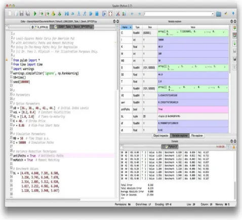
namely IPython and Spyder.
There is also Appendix A, on:
Best practices
Which best practices should I follow when developing Python code? The appendix
briefly reviews fundamentals of, for example, Python code syntax and
Python Deployment
This section shows how to deploy Python locally (or on a server) as well as via the web
browser.
Anaconda
A number of operating systems come with a version of Python and a number of additional
libraries already installed. This is true, for example, of Linux operating systems, which
often rely on Python as their main language (for packaging, administration, etc.).
However, in what follows we assume that Python is not installed or that we are installing
an additional version of Python (in parallel to an existing one) using the Anaconda
distribution.
You can download Anaconda for your operating system from the website
http://continuum.io/downloads. There are a couple of reasons to consider using Anaconda
for Python deployment. Among them are:
Libraries/packages
You get more than 100 of the most important Python libraries and packages in a
single installation step; in particular, you get all these installed in a version-consistent manner (i.e., all libraries and packages work with each other).[6]
Open source
The Anaconda distribution is free of charge in general,[7] as are all libraries and
packages included in the distribution.
Cross platform
It is available for Windows, Mac OS, and Linux platforms.
Separate installation
It installs into a separate directory without interfering with any existing installation; no root/admin rights are needed.
Automatic updates
Libraries and packages included in Anaconda can be (semi)automatically updated via
free online repositories.
Conda package manager
The package manager allows the use of multiple Python versions and multiple
versions of libraries in parallel (for experimentation or development/testing purposes); it also has great support for virtual environments.
After having downloaded the installer for Anaconda, the installation in general is quite
easy. On Windows platforms, just double-click the installer file and follow the instructions.
Under Linux, open a shell, change to the directory where the installer file is located, and
type:
Replacing the file name with the respective name of your installer file. Then again follow the instructions. It is the same on an Apple computer; just type:
$ bash Anaconda-1.x.x-MacOSX-x86_64.sh
making sure you replace the name given here with the correct one. Alternatively, you can use the graphical installer that is available.
After the installation you have more than 100 libraries and packages available that you can use immediately. Among the scientific and data analytics packages are those listed in Table 2-1.
Table 2-1. Selected libraries and packages included in Anaconda
Name Description
BitArray Object types for arrays of Booleans
CubesOLAP Framework for Online Analytical Processing (OLAP) applications
Disco mapreduce implementation for distributed computing
Gdata Implementation of Google Data Protocol
h5py Python wrapper around HDF5 file format
HDF5 File format for fast I/O operations
IPython Interactive development environment (IDE)
lxml Processing XML and HTML with Python
matplotlib Standard 2D and 3D plotting library
MPI4Py Message Parsing Interface (MPI) implementation for parallel computation
MPICH2 Another MPI implementation
NetworkX Building and analyzing network models and algorithms
NumPy Powerful array class and optimized functions on it
pandas Efficient handling of time series data
PyTables Hierarchical database using HDF5
SciPy Collection of scientific functions
Scikit-LearnMachine learning algorithms
Spyder Python IDE with syntax checking, debugging, and inspection capabilities
statsmodels Statistical models
SymPy Symbolic computation and mathematics
Theano Mathematical expression compiler
If the installation procedure was successful, you should open a new terminal window and should then be able, for example, to start the Spyder IDE by simply typing in the shell:
$ spyder
Alternatively, you can start a Python session from the shell as follows:
$ python
Python 2.7.6 |Anaconda 1.9.2 (x86_64)| (default, Feb 10 2014, 17:56:29) [GCC 4.0.1 (Apple Inc. build 5493)] on darwin
Type “help”, “copyright”, “credits” or “license” for more information. >>> exit()
$
Anaconda by default installs, at the time of this writing, with Python 2.7.x. It always
comes with conda, the open source package manager. Useful information about this tool
can be obtained by the command:
$ conda info
Current conda install:
platform : osx-64 conda version : 3.4.1
python version : 2.7.6.final.0
root environment : /Library/anaconda (writable) default environment : /Library/anaconda
envs directories : /Library/anaconda/envs package cache : /Library/anaconda/pkgs
channel URLs : http://repo.continuum.io/pkgs/free/osx-64/ http://repo.continuum.io/pkgs/pro/osx-64/ config file : None
is foreign system : False
conda allows one to search for libraries and packages, both locally and in available online
repositories:
$ conda search pytables Fetching package metadata: ..
pytables . 2.4.0 np17py27_0 defaults 2.4.0 np17py26_0 defaults 2.4.0 np16py27_0 defaults 2.4.0 np16py26_0 defaults . 3.0.0 np17py27_0 defaults 3.0.0 np17py26_0 defaults 3.0.0 np16py27_0 defaults 3.0.0 np16py26_0 defaults . 3.0.0 np17py33_1 defaults . 3.0.0 np17py27_1 defaults 3.0.0 np17py26_1 defaults . 3.0.0 np16py27_1 defaults 3.0.0 np16py26_1 defaults 3.1.0 np18py33_0 defaults * 3.1.0 np18py27_0 defaults 3.1.0 np18py26_0 defaults 3.1.1 np18py34_0 defaults 3.1.1 np18py33_0 defaults 3.1.1 np18py27_0 defaults 3.1.1 np18py26_0 defaults
The results contain those versions of PyTables that are available for download and
installation in this case and that are installed (indicated by the asterisk). Similary, the list
command gives all locally installed packages that match a certain pattern. The following lists all packages that start with “pyt”:
$ conda list ^pyt
# packages in environment at /Library/anaconda: #
pytables 3.1.0 np18py27_0 pytest 2.5.2 py27_0 python 2.7.6 1 python-dateutil 1.5 <pip> python.app 1.2 py27_1 pytz 2014.2 py27_0
More complex patterns, based on regular expressions, are also possible. For example:
$ conda list ^p.*les$
# packages in environment at /Library/anaconda: #
pytables 3.1.0 np18py27_0 $
Suppose we want to have Python 3.x available in addition to the 2.7.x version. The
package manager conda allows the creation of an environment in which to accomplish this
goal. The following output shows how this works in principle:
$ conda create -n py33test anaconda=1.9 python=3.3 numpy=1.8 Fetching package metadata: ..
Solving package specifications: .
Package plan for installation in environment /Library/anaconda/envs/py33test:
The following packages will be downloaded:
package | build –––––––––|–––––—
anaconda-1.9.2 | np18py33_0 2 KB …
xlsxwriter-0.5.2 | py33_0 168 KB
The following packages will be linked:
package | build –––––––––|–––––—
zlib-1.2.7 | 1 hard-link
Proceed ([y]/n)?
When you type y to confirm the creation, conda will do as proposed (i.e., downloading,
extracting, and linking the packages):
*******UPDATE**********
Fetching packages …
anaconda-1.9.2-np18py33_0.tar.bz2 100% |##########| Time: 0:00:00 173.62 kB/s …
xlsxwriter-0.5.2-py33_0.tar.bz2 100% |############| Time: 0:00:01 131.32 kB/s Extracting packages …
[ COMPLETE ] |##########################| 100% Linking packages …
[ COMPLETE ] |##########################| 100% #
# To activate this environment, use: # $ source activate py33test
#
# To deactivate this environment, use: # $ source deactivate
#
Now activate the new environment as advised by conda:
$ source activate py33test
discarding /Library/anaconda/bin from PATH
prepending /Library/anaconda/envs/py33test/bin to PATH (py33test)$ python
Python 3.3.4 |Anaconda 1.9.2 (x86_64)| (default, Feb 10 2014, 17:56:29) [GCC 4.0.1 (Apple Inc. build 5493)] on darwin
Type “help”, “copyright”, “credits” or “license” for more information. >>> print “Hello Python 3.3” # this shouldn’t work with Python 3.3 File “<stdin>”, line 1
print “Hello Python 3.3” # this shouldn’t work with Python 3.3 ^
SyntaxError: invalid syntax
>>> print (“Hello Python 3.3”) # this syntax should work Hello Python 3.3
>>> exit() $
Obviously, we indeed are now in the Python 3.3 world, which you can judge from the Python version number displayed and the fact that you need parentheses for the print
statement to work correctly.[8]
MULTIPLE PYTHON ENVIRONMENTS
With the conda package manager you can install and use multiple separated Python environments on a single
machine. This, among other features, simplifies testing of Python code for compatibility with different Python
versions.
Single libraries and packages can be installed using the conda install command, either
in the general Anaconda installation:
$ conda install scipy
or for a specific environment, as in:
$ conda install -n py33test scipy
Here, py33test is the environment we created before. Similarly, you can update single
packages easily:
$ conda update pandas
dependencies for which no current version is installed. For our newly created environment, the updating would take the form:
$ conda update -n py33test pandas
Finally, conda makes it easy to remove packages with the remove command from the main
installation or a specific environment. The basic usage is:
$ conda remove scipy
For an environment it is:
$ conda remove -n py33test scipy
Since the removal is a somewhat “final” operation, you might want to dry run the command:
$ conda remove —dry-run -n py33test scipy
If you are sure, you can go ahead with the actual removal. To get back to the original
Python and Anaconda version, deactivate the environment:
$ source deactivate
Finally, we can clean up the whole environment by use of remove with the option —all:
$ conda remove —all -n py33test
The package manager conda makes Python deployment quite convenient. Apart from the
basic functionalities illustrated in this section, there are also a number of more advanced features available. Detailed documentation is found at http://conda.pydata.org/docs/.
Python Quant Platform
There are a number of reasons why one might like to deploy Python via a web browser.
Among them are:
No need for installation
Local installations of a complete Python environment might be both complex (e.g., in
a large organization with many computers), and costly to support and maintain; making Python available via a web browser makes deployment much more efficient
in certain scenarios.
Use of (better) remote hardware
When it comes to complex, compute- and memory-intensive analytics tasks, a local computer might not be able to perform such tasks; the use of (multiple) shared
servers with multiple cores, larger memories, and maybe GPGPUs makes such tasks possible and more efficient.
Collaboration
Working, for example, with a team on a single or multiple servers makes
collaboration simpler and also increases efficiency: data is not moved to every local machine, nor, after the analytics tasks are finished, are the results moved back to some central storage unit and/or distributed among the team members.
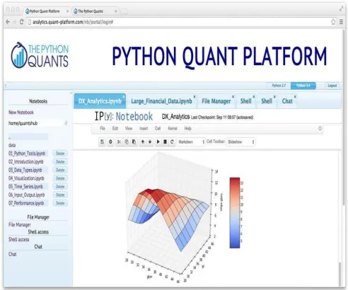
The Python Quant Platform is a web- and browser-based financial analytics and
register for the platform at http://quant-platform.com. It features, among others, the following basic components:
File manager
A tool to manage file up/downloads and more via a web GUI.
Linux terminal
A Linux terminal to work with the server (for example, a virtual server instance in the
cloud or a dedicated server run on-premise by a company); you can use Vim, Nano,
etc. for code editing and work with Git repositories for version control. Anaconda
An Anaconda installation that provides all the functionality discussed previously; by
default you can choose between Python 2.7 and Python 3.4.
Python shell
The standard Python shell.
IPython Shell
An enhanced IPython shell. IPython Notebook
The browser version of IPython. You will generally use this as the central tool.
Chat room/forum
To collaborate, exchange ideas, and to up/download, for example, research documents.
Advanced analytics
In addition to the Linux server and Python environments, the platform provides
analytical capabilities for, e.g., portfolio, risk, and derivatives analytics as well as for backtesting trading strategies (in particular, DX analytics; see Part III for a simplified
but fully functional version of the library); there is also an R stack available to call,
for example, R functions from within IPython Notebook.
Standard APIs
Standard Python-based APIs for data delivery services of leading financial data
providers.
When it comes to collaboration, the Python Quant Platform also allows one to define —
under a “company” — certain “user groups” with certain rights for different Python
Tools
The success and popularity of a programming language result to some extent from the tools that are available to work with the language. It has long been the case that Python
was considered a nice, easy-to-learn and easy-to-use language, but without a compelling set of tools for interactive analytics or development. This has changed. There are now a large number of tools available that help analysts and developers to be as productive as possible with Python. It is not possible to give even a somewhat exhaustive overview.
However, it is possible to highlight two of the most popular tools in use today: IPython
and Spyder.[9]
Python
For completeness, let us first consider using the standard Python interpreter itself. From
the system shell/command-line interface, Python is invoked by simply typing python:
$ python
Python 2.7.6 |Anaconda 1.9.2 (x86_64)| (default, Feb 10 2014, 17:56:29) [GCC 4.0.1 (Apple Inc. build 5493)] on darwin
Type “help”, “copyright”, “credits” or “license” for more information. >>> print “Hello Python for Finance World.”
Hello Python for Finance World. >>> exit()
$
Although you can do quite a bit of Python with the standard prompt, most people prefer to
use IPython by default since this environment provides everything that the standard
interpreter prompt offers, and much more on top of that.
IPython
IPython was used in Chapter 1 to present the first examples of Python code. This section
gives an overview of the capabilities of IPython through specific examples. A complete
ecosystem has evolved around IPython that is so successful and appealing that users of
other languages make use of the basic approach and architecture it provides. For example, there is a version of IPython for the Julia language.
From shell to browser
IPython comes in three flavors:
Shell
The shell version is based on the system and Python shell, as the name suggests;
there are no graphical capabilities included (apart from displaying plots in a separate window).
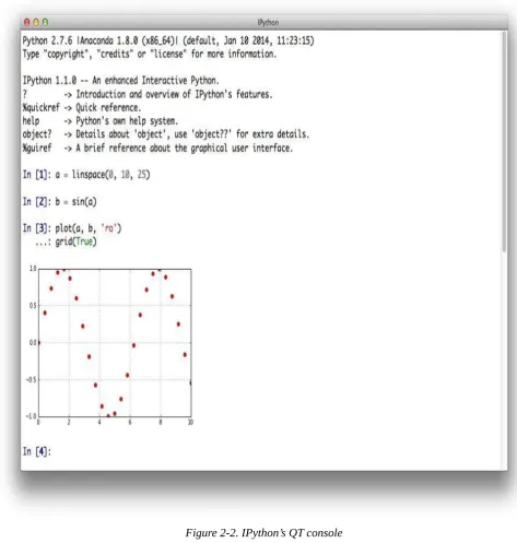
QT console
This version is based on the QT graphical user interface framework (cf.
http://qt-project.org), is more feature-rich, and allows, for example, for inline graphics.
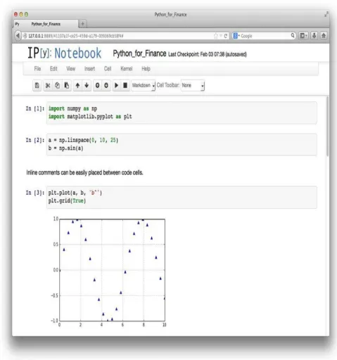
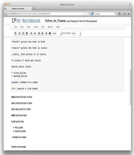
Notebook
This is a JavaScript-based web browser version that has become the community