promoting access to White Rose research papers
White Rose Research Online
Universities of Leeds, Sheffield and York
http://eprints.whiterose.ac.uk/
This is an author produced version of a paper published in Computers & Graphics.
White Rose Research Online URL for this paper: http://eprints.whiterose.ac.uk/3553/
Published paper
Progressive Refinement Rendering
of Implicit Surfaces
Manuel N. Gamito
1, Steve C. Maddock
Department of Computer Science, The University of Sheffield
Abstract
The visualisation of implicit surfaces can be an inefficient task when such surfaces are complex and highly detailed. Visualising a surface by first converting it to a polygon mesh may lead to an excessive polygon count. Visualising a surface by direct ray casting is often a slow procedure. In this paper we present a progressive refinement renderer for implicit surfaces that are Lipschitz continuous. The renderer first displays a low resolution estimate of what the final image is going to be and, as the computation progresses, increases the quality of this estimate at an interactive frame rate. This renderer provides a quick previewing facility that significantly reduces the design cycle of a new and complex implicit surface. The renderer is also capable of completing an image faster than a conventional implicit surface rendering algorithm based on ray casting.
Key words: Progressive refinement; Ray casting; Implicit surfaces; Lipschitz bounds
1 Introduction
Implicit surfaces find application in many areas of Computer Graphics where objects exhibiting complex topologies, i.e. with many holes or disconnected pieces, need to be modelled. An implicit surface is defined as the set of all pointsx∈R3
that verify the conditionf(x) = 0 for some functionf :R3
→R. Modelling with implicit surfaces amounts to the construction of an appropriate functionf, called theimplicit function, that will generate the desired surface. Over the years, three main strategies for the design of implicit functions have
1
become established. Algebraic surfaces arise from the use of polynomial impli-cit functions [1]. Sums of radial basis functions are also a popular method of constructing implicit surfaces. Depending on the choice of radial basis func-tion, these can be calledblobby models [2], metaballs [3] orsoft objects [4]. By carefully selecting the weights associated with each radial basis function, it is also possible to have an interpolating implicit surface that is constrained to pass through a set of scattered data points [5, 6]. Finally,hypertextures are an example of implicit functions that are generated by perturbing the surface of an initially smooth object with a combination of procedural noise functions [7]. By summing together many such noise functions a fractal hypertexture can be generated, having an associated fractal dimension.
Rendering algorithms for implicit surfaces can be broadly divided into meshing algorithms and ray casting algorithms. Meshing algorithms convert an impli-cit surface to a polygonal mesh format, which can be subsequently rendered in real time with modern graphics processor boards [8–10]. Ray casting al-gorithms bypass mesh generation entirely and compute instead the projec-tion of an implicit surface on the screen by casting rays from each pixel into three-dimensional space and finding their intersection with the surface [11– 13]. We propose an extension to ray casting algorithms for implicit surfaces that incorporates a progressive refinement rendering principle. The idea of progressive refinement for image rendering was first formalised in 1986 [14]. Progressive refinement rendering has received much attention in the fields of radiosity and global illumination [15, 16]. Progressive refinement approaches to volume rendering have also been developed [17, 18]. Our implicit surface renderer uses progressive refinement to visualise an increasingly better approx-imation to the final implicit surface. It allows the user to make quick editing decisions without having to wait for a full ray casting solution to be computed. Because the algorithm is progressive, the rendering can be terminated as soon as the user is satisfied or not with the look of the surface. The renderer can also be interactively controlled by the user through the specification of image regions. Image refinement will only occur inside a region, once the region be-comes active, while the remainder of the image is kept on hold. In this way the user can steer the application into rendering image regions that he considers to be more interesting or troublesome.
Our method is able to render any implicit surface whose generating functionf
is Lipschitz continuous. For a function to be Lipschitz continuous there must exist a real number λ such that:
|f(xa)−f(xb)|< λkxa−xbk for anyxa,xb ∈R
3
. (1)
of the progressive refinement algorithm towards the final image depends on the value ofλthat has to be provided beforehand and is specific to the partic-ular implicit function being visualised. If the Lipschitz constant off is known, the algorithm will have optimal convergence. Otherwise, a Lipschitz bound must be provided, with the algorithm exhibiting slower convergence the lar-ger the value of λ is. Values of λ smaller than the Lipschitz constant can also be attempted to increase the convergence rate at the price that surface visualisations are no longer guaranteed to be correct. Most implicit surfaces of interest in Computer Graphics are continuous, which implies that they are Lipschitz continuous also. The application of the progressive refinement ren-derer to Lipschitz continuous surfaces only is, therefore, not overly restrictive. Examples of surfaces that cannot be rendered with our proposed method can be found mainly within some types of algebraic surfaces, which contain isol-ated points where the surface gradient is infinite.
The main stage of our method consists in the subdivision of the image space into progressively smaller square samples. Information about the part of the implicit function that is visible through a sample is obtained by shooting a ray through the centre of the sample and marching towards the surface intersec-tion point with the help of a guaranteed ray-surface intersecintersec-tion algorithm [13]. The surface Lipschitz bound is used to compute step lengths that bring the ray progressively closer to the surface. Projecting the area of a sample from the viewpoint and into object space defines the sample’s view volume, which features the ray along its main axis. We enhance the surface intersection al-gorithm by testing for intersections inside the whole view volume of the sample whose ray is being traced. As we march along a ray towards the surface there comes a distance after which it is no longer possible to guarantee that no in-tersections occur inside the view volume that is defined around the ray. At this point, sample subdivision takes place and new rays are shot, each surrounded by a thinner view volume. The sample subdivision mechanism stops once a sample has reached pixel size, at which point conventional ray casting is used to march along the remainder of the distance towards the surface.
Section 2 describes previous work that provides previewing facilities for im-plicit surfaces. Some of the work described in that section was not developed with quick previewing in mind but it can be used to that effect. Section 3 describes our progressive refinement previewer. Although our main research focus is in the area of procedural landscape modelling with hypertextured surfaces, we shown in Section 4 progressive refinement rendering examples for the three main categories of implicit surfaces: algebraic surfaces, surfaces gen-erated from sums of radial basis functions and hypertextures. A performance comparison is also presented between our previewer and a standard rendering algorithm for implicit surfaces based on ray casting. Section 5 presents our conclusions. Appendix A describes an extension of the progressive refinement algorithm to incorporate anti-aliasing.
2 Previous Work
One of the best known techniques for previewing implicit surfaces at interact-ive frame rates is based on the dynamic placement of discs that are tangent to the surface [19, 20]. The discs are kept apart by the application of repulsive forces and are constrained to remain on the surface. Each disc is also made tangent to the surface by sharing the surface normal at the point where it is located. This previewing system relies on a characteristic of our visual system whereby we are able to infer the existence of an object based solely on the distribution of a small number of features on the surface of that object [21]. This visual trait only works, however, when the surface of the object is simple and fairly smooth. If the surface is irregular, as in the case of a fractal hyper-texture, a random distribution of discs is visible and no object is perceived.
Instead of performing object space subdivision, one can also perform image space subdivision in order to obtain a progressive rendering mechanism. Im-age space subdivision provides a general approach to progressive refinement rendering and can be used for any rendering problem, not only for the visual-isation of implicit surfaces. Sample subdivision in image space was originally proposed as an anti-aliasing method for ray tracing [25]. Four rays are shot at the corners of each rectangular sample. If the computed colours for these rays differ by more than some specified amount, the sample is subdivided into four smaller samples and more rays are shot through the corners of the new samples. This type of image space subdivision can also be used for progressive refinement previewing by Gouraud shading the interior of each sample based on the colours at its corners. As the samples become progressively smaller, the image converges to the correct rendering solution. Such a previewing tool was implemented as part of the Rayshadepublic domain ray tracer [26].
Rather than simply comparing the colours at the corners of a sample, more sophisticated approaches to image space subdivision have been proposed as part of a ray tracing algorithm [27, 28]. These approaches feature a stochastic distribution of rays that are shot around each image sample. By performing a probabilistic analysis on the colours returned by these rays, it is possible to make a decision with a desired degree of confidence on whether the sample should be subdivided or not. These probabilistic subdivision methods have also been extended to distributed ray tracers running on massively parallel computers [29]. There are two problems associated with probabilistic image subdivision methods. One problem is that the decision to subdivide a sample is entirely dependent on the information returned by a discrete set of rays. Because this discrete set is only an approximation to a continuous image dis-tribution, wrong subdivision decisions can sometimes occur. This often leads to small objects being missed by the progressive ray tracer. The other prob-lem is that subdivision techniques in image space do not take into account any information about the surface that is being rendered. They only look at colour information on the image plane. The subdivision of a sample causes new rays to be shot that do not take advantage of any surface information that may have been gathered whilst tracing rays that originated earlier in the subdivision process.
In that work, affine arithmetic was used to compute bounds for the impli-cit function. Affine arithmetic provides an automatic method of computing bounds for arbitrary functions but it is slower than using a Lipschitz based method. The use of Lipschitz methods for ray casting, on the other hand, re-quires that at least a Lipschitz bound be known about the implicit function. Such Lipschitz bounds for many types of implicit functions are available in the literature [11, 13].
3 Progressive Refinement Rendering
Progressive refinement rendering of implicit surfaces proceeds by subdividing the image space into increasingly smaller samples. We use the term “sample” in this context to refer to square partitions of the image space with arbitrary size. A sample always corresponds to a n×n set of pixels on the screen so that the boundary of the sample coincides with the boundary of that square array of pixels. As samples are subdivided, the sizenin pixels of newer samples progressively decreases. The smallest samples used by the progressive renderer are sized 1×1 and correspond exactly to the screen extent of just one pixel.
The portion of the scene that is visible through a sample defines a quadrilateral pyramid with the apex located at the viewpoint. Shooting such pyramidal rays through each image pixel has previously been proposed as a technique to perform anti-aliasing and to compute fuzzy reflections and shadows [31]. For simplicity of implementation, however, we use cones rather than pyramids to enclose the space visible through each sample. In this respect, our algorithm has similarities with cone tracing as we shoot cones into the scene and check their intersection with the surface [32]. The difference with the original cone tracing algorithm is that, rather than compute a visibility coverage mask that is used to perform anti-aliasing, we choose to subdivide samples and therefore make the cones progressively thinner as they get closer to the surface. This is so that we can guarantee that no surface intersection will occur inside the cone up to some maximum distance. As the distance travelled along a cone approaches the intersection distance to the surface, this guarantee can only be provided if the aperture angle of the cone is made smaller. Having stressed this difference, we continue to refer to “cone tracing” as the process of shooting a cone through a square sample and into the scene.
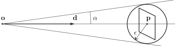
PSfrag
α
ǫ
[image:8.612.138.438.73.153.2]o d p
Fig. 1. The geometry of a cone that encloses the space visible through a sample.
(1) Trace cone through the sample up to a maximum distance.
(2) Render the sample by evaluating the shading model at the point of max-imum distance along the axis of the cone.
(3) If the sample is larger than a pixel, subdivide it and append the children to the end of the queue.
A ray-surface intersection algorithm, rather than the cone tracing algorithm, is used for samples that have reached pixel size [13]. The parts of the image that are covered by these samples receive their final colour in step (2), as explained above, and are no longer affected by subsequent iterations. The progressive renderer finishes when the queue becomes empty. Once this happens the image will have reached its best quality. The final image is exactly equal to that which would have been obtained by conventional ray casting. This is because the final pixel colours are obtained by ray casting through the centre of each pixel along the distance that still needs to be travelled toward the surface.
3.1 Cone Tracing
Consider a sample with dimensions n∆l×n∆l where n×n is, as before, the number of pixels contained by the sample and ∆l is the lateral size of a pixel, measured along the image plane. The sample is centred at the point p on the image plane and we trace a cone through it with the apex placed at the camera’s viewpointo. Figure 1 exemplifies this geometry. The axis of the cone is a parametric ray defined as:
r(t) =o+td, (2)
where the normalised direction vector isd= (p−o)/kp−ok. The aperture of the cone is an angleα large enough to encompass all the scene visible through the sample. For the purpose of finding this angle, the smallest bounding sphere that encloses the sample is used. The radius of the bounding sphere is given by ǫ= 0.5√2n∆l and the aperture angle is:
α= tan−1 ǫ
The cone is traced through the scene by stepping along the axis r with step lengths that are guaranteed not to cause intersection with the implicit sur-face. Such a guarantee is provided by the Lipschitz bound of the surface generating function f. Applying the definition (1) of Lipschitz continuity to the cone-surface intersection problem, it is possible to show that the se-quence of steps along the axis of the cone expressed by the iterative equation
ti+1 = ti +|f(r(ti)|/λ either converges to the intersection point or diverges,
the latter case occurring when the axis does not intersect with the implicit surface [13]. For every iteration of the cone tracing procedure there is a sphere centred at the point r(ti) and with radius|f(r(ti)|/λthat encloses a region of space known to be completely outside the surface. As the tracing procedure converges towards the intersection point, these spheres become smaller and more densely packed.
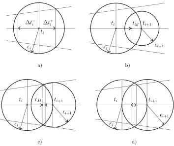
[image:9.612.218.367.618.684.2]Tracing along the axis r(t) can only proceed while the sequence of bounding spheres encloses the cone. There is a maximum distance tM after which parts of the cone begin to fall outside the union of all the spheres. It is known with certainty that for ti 6 tM no intersection between the cone and the implicit surface has occurred. For ti > tM this certainty no longer exists and cone tracing for the current sample must be terminated. The tracing will proceed for distances larger than tM after the sample has been subdivided and cones with smaller angles of aperture have been generated. The smaller cones that result from the subdivision will then start tracing fromtM.
Figure 2 shows several situations that occur as part of the cone tracing pro-cedure. Let ǫi =|f(r(ti))|/λbe the radius of the sphere that is centred on the point r(ti) for the distance ti along the cone axis. Figure 2a) shows that any individual sphere must be large enough to bound the cone in the neighbour-hood of its centre atr(ti). This is true if the radius of the sphere is larger than the radius of the section of the cone at ti:
ǫi > titanα. (4)
Once condition (4) is verified, it is possible to define two positive offsets ∆t−
i
and ∆t+
i , relative to ti, that give the neighbourhoodti−∆t
−
i 6ti 6ti+ ∆t
+
i
where the sphere is known to bound the cone. Inside this range of distances, it is guaranteed that no intersections with the implicit surface will exist. The two offsets are given by:
∆t−
i =δ+tisin
2
α and (5a)
∆t+
i =δ−tisin
2
α, with (5b)
δ=qǫ2
i cos2α−t
2
i sin
2
α. (5c)
ti
∆t+
i
∆t−
i
ǫi
a)
ti tM ti+1
ǫi ǫi+1
b)
ti tM ti+1
ǫi
ǫi+1
c)
ti ti+1
ǫi
ǫi+1
[image:10.612.111.465.78.375.2]d)
Fig. 2. Several configurations that may arise while performing cone tracing.
Figures 2b) to 2d) illustrate the three situations that can arise when marching from the sphere atti to the next sphere atti+1. In Figure 2b), the next sphere
is not large enough to verify (4). In this case, cone tracing must stop at the current sphere with radiusǫi and the maximum distance that can be travelled along the cone istM =ti+ ∆t+
i . In Figure 2c), the sphere at ti+1 satisfies (4)
but there is still a small part of the cone that falls outside the union of the two spheres. This situation can be detected by the condition:
ti+1−ti < ∆t
−
i+1+ ∆t
+
i . (6)
If (6) does not hold then again the sphere at ti+1 must be ignored, with the
distance tM being given as in the previous case. Finally, in Figure 2d), cone tracing can proceed from ti to ti+1 with the testing of subsequent spheres.
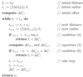
Figure 3 shows the cone tracing algorithm in pseudo-code form. The cone is traced from a starting distance t0 up to a large enough distance t∞ so that any valid intersections are known to be inside the interval [t0, t∞]. The distance t∞ is usually found by performing a quick intersection test between the cone and a bounding sphere that surrounds the whole implicit surface. The algorithm returns the maximum distancetM that can be traced along the cone. Within the interval [t0, tM] there are no intersections with the surface.
ti :=t0; // initial distance
ǫi := |f(r(t0))|/λ; // initial radius
compute ∆t+
i ; // initial offset
while ti < t∞ do
ti+1 :=ti +ǫi; // next distance
ǫi+1 :=|f(r(ti+1))|/λ; // next radius
if ǫi+1 < ti+1tanα // condition (4) return ti + ∆t+
i ;
compute ∆t−
i+1 and ∆t +
i+1; // equations (5) if ti+1−ti < ∆t
−
i+1 + ∆t
+
i // condition (6)
return ti + ∆t+i ;
ti :=ti+1; // take step
ǫi := ǫi+1;
∆t+
i := ∆t
+
i+1;
[image:11.612.156.440.69.332.2]return ti;
Fig. 3. The cone tracing algorithm in pseudo-code format.
then the surface is not intersected along the whole extent of the cone. One necessary prerequisite for the cone tracing algorithm to work is that condition (4) must hold for the initial sphere placed att0. If the condition is not verified,
the sample to which the cone belongs will have to be subdivided, with no cone tracing actually occurring. This is handled as part of the sample subdivision process, as explained in Section 3.3. The offsets ∆t−
i+1and ∆t +
i+1are computed
simultaneously with equations (5) even though ∆t+
i+1 will only be required
during the subsequent iteration, when it becomes ∆t+
i . This is more efficient
than computing ∆t+
i and ∆t
−
i+1 independently for every iteration.
3.2 Cone Rendering
Once cone tracing terminates, with the computation of the distance tM, the sample through which the cone was shot is painted on the screen. The colour for this sample is obtained by evaluating some appropriate shading model, which, from the point of view of the progressive refinement algorithm, is re-garded as a generic function s(x,n,v) that returns a colour at the point x
The shading model can be evaluated at any point in space and not only for points on the implicit surface. During the cone tracing process, the rays that constitute the axes of the cones have not yet reached the surface and so shading values are being computed that do not correspond to the cor-rect shading or geometry of the surface. For any given cone, the evaluation of the shading model s(x,n,v) corresponds to shading an implicit surface given by {x ∈ R3
: ˜f(x,r(tM)) = 0}, where the new implicit function is ˜
f(x,r(tM)) = f(x)−f(r(tM)). The function ˜f generates a surface that is larger than the one generated by f. In fact, it is possible to show that the correct implicit surface is completely enclosed by the surface generated from
˜
f, given that f(x) andf(r(tM)) have the same sign when evaluated at points
x and r(tM) outside the surface. As cone tracing progresses and newer cones get closer to the surface, the termf(r(tM)) vanishes with the consequence that
˜
f → f and the shading values converge towards the correct shading of the surface. This progression, in visual terms, corresponds to a gradual shrinking of the perceived surface, with the surface finally settling on its correct shape at the completion of the progressive rendering algorithm.
The painting of a sample on the screen is done with a uniform colour that corresponds to the shading value of the point at the centre of the sample, since it is through this point that the axis of the cone passes. While painting the square region of the screen that corresponds to a sample, the previous colour that was stored in that region is overwritten by the new colour. The previous colour was obtained when painting the parent sample. Through this procedure, the screen buffer is constantly being refreshed with new shading data as subdivision of the samples progresses.
3.3 Sample Subdivision
The subdivision of samples requires that the width and height of the image in pixels be first decomposed into a product of prime numbers. In this way, it becomes possible to know, at each level of subdivision, how a given sample should be split so that the newer samples still correspond to an integer number of pixels on the screen. For an image with a resolution of m×n pixels, the prime number factorisation results in:
m=u pk1
1 p
k2
2 . . . p
kn
n , (7a)
n=v pk1
1 p
k2
2 . . . p
kn
n , (7b)
where u = m/gcd (m, n), v = n/gcd (m, n) and gcd (m, n) is the greatest common divisor betweenmandn. The sequence of prime factorsp1, p2, . . . , pn
tMi−1
t0i
di
[image:13.612.166.412.83.189.2]di−1
Fig. 4. A child cone shown in relation to its parent cone as part of the sample subdivision process.
size. If m =n, in particular, then u= v = 1 and the image corresponds to a single top level sample. For a 800×600 image, to give an example of the more general rectangular image case, we havem = 4×52
×23
and n= 3×52
×23
. The queue of samples used by the progressive refinement algorithm, in this case, is initialised with 4×3 top level samples with a resolution of 200×200 pixels each. At the first level of subdivision, every top level sample is then subdivided into 5×5 samples with a resolution of 40×40 pixels each. The optimal image subdivision scenario occurs with square images that have a resolution of 2k×2k, for some k >0, where every sample is always subdivided
into 2×2 smaller samples. The worst scenario occurs when either m or n is a prime number, in which case it becomes impossible to perform any further prime factorisation. The progressive refinement algorithm is then initialised withm×n top level samples with the consequence that the subdivision stage is skipped and the algorithm goes straight to the final ray casting stage that occurs at the pixel level.
The generation of new cones is part of the sample subdivision process. Figure 4 shows how one of thepi×pi child cones is generated after its parent cone was traced, where pi is the prime factor at subdivision level i. The unit direction vector di of the child cone is the one that goes from the camera’s viewpoint
through the centre point of the child sample. The initial distancet0i along the
child cone is:
t0i =tMi
−1/(di·di−1), (8) wheredi−1 is the unit direction vector of the parent cone. Equation (8) makes
the child cone start off from a point that lies in the plane orthogonal to the parent cone at tMi−1. The aperture angle of the child cone is given by (3) and is always smaller than the aperture angle of the parent cone. If the child cone does not verify condition (4), it is further subdivided into pi+1 ×pi+1
3.4 Specifying Regions of Interest
A user can interactively influence the rendering algorithm by drawing a rectan-gular region of interest (ROI) over the image. The algorithm will then refine the image only inside the specified region. This is accomplished by creat-ing a secondary queue that stores the samples that are relevant to the ROI. When the user finishes drawing the region, the primary queue is scanned and all samples that intersect with the rectangle corresponding to that ROI are transferred to the secondary queue. The algorithm then proceeds as explained before with the difference that the secondary queue is now being used. Once this queue becomes empty, the portion of the image inside the ROI is fully rendered and the algorithm returns to subdividing the samples that were left in the primary queue. It is also possible to cancel the ROI at any time by flushing any samples still in the secondary queue back to the primary queue.
3.5 Some Remarks on Implementation
The best implementation strategy for our rendering method is to have two threads running concurrently: a refinement thread and a display thread. The two threads communicate through an image buffer. The refinement thread requires write access to the buffer as it continuously draws coloured squares onto it that correspond to the samples whose cones have finished being traced. The display thread only requires read access to the same buffer. No mutual exclusion mechanisms need to be enforced between the two threads. It may happen that the display thread will read some part of the image buffer in an incoherent state because of a simultaneous write by the refinement thread but any display errors that may occur will be erased during the next display refresh.
The display thread is controlled by a timer that ensures a constant frame rate. The thread remains in a sleep state except for the periodical invocation of the timer handler routine. The main function of this timer handler is to invoke a graphics library call that transfers the content of the image buffer, handled by the application, to the hardware frame buffer, handled by the machine’s GPU. The display thread is also responsible for the interactive editing of regions of interest and notifying the refinement thread to the existence of such regions.
4 Results and Discussion
Figures 5, 6 and 7 show four snapshots each, taken during the progressive refinement rendering of three different types of implicit surfaces. All snap-shots were rendered with a resolution of 800×800 pixels. The snapshots were obtained at the transition point between two levels of subdivision in the im-age, i.e. when all the samples at one level have been processed and before processing any of the samples at the next lower levels.
The algebraic surface shown in Figure 5 was first presented by Mitchell to demonstrate his robust ray casting based on interval arithmetic [12]. The im-plicit function for Mitchell’s surface is:
f(x, y, z) = 4x4
+ (y2
+z2
)2
+ + 17x2
(y2
+z2
)−20(x2
+y2
+z2
) + 17. (9)
The Lipschitz constant of (9), when considered overR3
, is infinite. The surface, however, is known to exist inside a cube with dimensions [−2,2]×[−2,2]× [−2,2]. The Lipschitz constant off(x, y, z) becomes finite when evaluated over this subdomain only.
Figure 6 shows a model that was made to resemble a figure in a painting by Dali. The implicit surface for this model is a sum of sixty radial basis functions:
f(x) = 0.5−
60
X
i=1
sip(kx−xik/Ri), (10)
where si is the strength, Ri is the radius and xi is the position of each basis
function. The factor 0.5 is the surface threshold. The basis function p is a polynomial with a compact support in the range [0,1], veryfing p(0) = 1 and
p(1) = 0. The evaluation of the implicit function for any pointxthat is outside the support of all the basis functions returns the constant value f(x) = 0.5. Shading computations cannot be properly performed in this outside region because ∇f(x) = 0. To overcome this problem, we modified (10) to return
f(x) = 0.5 +kx−xik −Ri for points where f(x) would have been equal to
0.5 otherwise and where xi and Ri are related to the basis function that is
closest to x. With this modification, the surface appears in the early stages of the progressive visualisation as a union of spheres of different radii, where each sphere is centred at one of the xi points. It must be mentioned that
Fig. 5. From left to right, top to bottom, snapshots taken during the progressive refinement rendering of an algebraic surface. The snapshots were taken after 626, 8 178, 107 862 and 410 590 iterations, respectively. The wall clock times at each snapshot are 0.35s, 0.71s, 5.71s and 19.18s, respectively.
It is possible to improve the rendering time for the model of Figure 6 by first clipping every cone against the bounding spheres of radiiRi that represent the support of each basis function. As a consequence, the distance along the cone is partitioned into disjoint intervals where only a small set of basis functions in-fluence each particular interval. This optimisation was first proposed to speed up the ray tracing of soft objects and can be extended to our cone tracing technique with little difficulty [4]. It makes the evaluation of (10) much more efficient since it is not necessary to iterate over all the sixty basis functions for every function call. Localised Lipschitz bounds can also be used inside each interval, reflecting only the basis functions that contribute to that interval and providing further improvement to the convergence rate of the renderer.
Figure 7 shows a hypertextured sphere of unit radius generated with:
Fig. 6. From left to right, top to bottom, snapshots taken during the progressive refinement rendering of a blobby model. The snapshots were taken after 13 151, 53 151, 163 851 and 298 467 iterations, respectively. The wall clock times at each snapshot are 2.56s, 18.41s, 1m 17.11s and 2m 39.48s, respectively.
The term kxk − 1 produces the spherical shape and n(x) is a procedural gradient noise function that introduces the hypertextured detail [33]. The amplitude 0.8 controls the height of the procedural detail while the scaling
n(4x) controls the size of the detail features relative to the size of the sphere.
Fig. 7. From left to right, top to bottom, snapshots taken during the progressive refinement rendering of a hypertextured surface. The snapshots were taken after 3 103, 10 755, 31 279 and 327 295 iterations, respectively. The wall clock times at each snapshot are 0.45s, 0.90s, 2.10s and 23.22s, respectively.
Table 1
Statistics for Figures 5, 6 and 7 with three different rendering methods.
Previewer Optimised R.C. Standard R.C.
Time # Evals Time # Evals Time # Evals Fig. 5 19.18s 26 803 413 14.03s 30 701 240 19.87s 44 895 932
Fig. 6 2m39.48s 30 563 596 4m47.56s 58 132 753 6m59.27s 84 760 569
Fig. 7 23.22s 12 641 154 29.69s 21 425 128 36.69s 27 504 354
To test the performance of the progressive refinement renderer with increas-ingly complex surfaces, we modified the hypertexture example of Figure 7 to sum the contribution of several layers of procedural noise:
f(x) = kxk −1 + 0.8
L−1
X
i=0
2−0.8in(2i+2
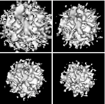
[image:18.612.101.487.527.621.2]Fig. 8. A hypertexture with (from left to right) two to five layers of procedural gradient noise.
1 2 3 4 5
0 200 400 600 800 1000 1200
Layers
Rendering Time (s)
Progressive Refinement Optimised Ray Casting Standard Ray Casting
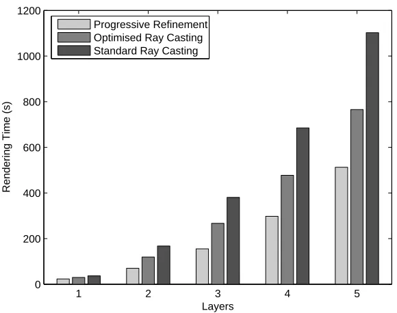
Fig. 9. Comparison between the total rendering times between our progressive re-finement previewer, a ray caster based on Lipschitz bounds and the same ray caster with an optimised overshooting factor.
The expression for the implicit function accumulatesLcopies of the procedural noise function whose basic frequencies follow a geometric sequence [35]. The caseL= 1 corresponds to the implicit function (11) that is shown in Figure 7. In the limit of an infinite number of layers, the surface would have a fractal dimension of 2.2. Hypertextured surfaces with theLparameter in (12) ranging from 2 to 5 are shown in Figure 8. The bar chart shown in Figure 9 compares the total rendering times of these increasingly more complex surfaces.
[image:19.612.136.426.225.454.2]tracing procedure, thereby reducing the number of evaluations of the implicit function. For most cases, this leads to a reduction of the total rendering time as shown by the previous results. If, however, the implicit function is very simple and can be evaluated quickly, the previewer can no longer compensate for the extra progressive refinement costs compared to a ray casting algorithm. This is the case of the algebraic surface of Figure 5, as shown in Table 1, where it takes longer to do progressive refinement even though the number of eval-uations of the implicit function with previewing is still the smallest for the three rendering methods.
Figure 10 shows three frames, with a resolution of 800×400 pixels, taken during the rendering of a procedural landscape. This landscape uses a combination of gradient noise, sparse convolution noise and cellular texture noise [33, 36, 37]. The faceted aspect of the terrain, in particular, is a characteristic of the spatial Voronoi decomposition performed by the cellular texture noise function. A region of interest (ROI), shown as a white rectangle, was used to focus the rendering on one of the terrain features. The top frame shows the image at the moment when the ROI was specified. The rendering time for this frame is 2m 15.09s. The middle frame shows the image at the moment when rendering inside the ROI was completed. The rendering time is now 4m 0.93s. The portion of the terrain inside the ROI has become fully resolved while the remaining terrain has not suffered any change since the previous frame. The bottom frame shows the final rendering, which is achieved after 14m 42.47s. The same landscape took 17m 13.26s to render with an optimised ray caster. The top frame demonstrates again how an approximate and quite acceptable rendering of the surface is available early during the rendering, in this case after 15% of the total rendering time has elapsed. During the course of some editing task, the user may be interested in resolving only the portion of the terrain that is contained by the ROI. In that case, he will achieve the most accurate results with only 27% of the total rendering time. The time necessary to resolve the ROI depends on its size and also on its placement over the image. Portions of the image that are closer to the horizon take longer to resolve since cones must be traced over a greater distance.
5 Conclusions
more flexible rendering approach offered by our previewer allows the user to make quick editing decisions about the surface. The previewer runs faster than straightforward ray casting for surfaces that are generated from complex im-plicit functions. It becomes slower than ray casting if the imim-plicit function is simple and can be evaluated efficiently because of the overheads required for progressive refinement. This is not a limitation since simple functions that can be rendered quickly with ray casting do not really need a previewing facility.
Sample subdivision is based on a prime number factorisation of the image resolution so that any subdivided sample always corresponds to an integer number of pixels on the screen. This technique works best for square images with a power of two resolution since, compared to images of similar size, it leads to the greatest number of subdivision levels. For images with a width or height that are prime numbers, no progressive refinement is possible and the algorithm automatically switches to ray casting. The interactive placement of regions of interest, however, still remains functional in these circumstances.
The use of guaranteed Lipschitz bounds during both the cone tracing and the ray casting stages of the progressive refinement algorithm means that no surface details with sizes that are above the size of a pixel can possibly be missed. This is an improvement over more general image space progressive refinement algorithms where small surfaces can sometimes escape detection. Surface components that are smaller than a pixel may still be rendered in-correctly, considering that only one ray is shot for each pixel at the highest level of subdivision. This problem can be solved with the implementation of an anti-aliasing technique.
A Anti-Aliasing
Because our aim was to provide an interactive and progressive refinement previewer for implicit surfaces, anti-aliasing was not an issue. Anti-aliasing, however, can be easily added to the rendering algorithm that we have de-veloped. Anti-aliasing is achieved by the process of filtering rectangular image regions that have constant luminous intensity [27]. All samples must be sub-divided down to a specified minimum size, which can be several times smaller than the size of a pixel. Let the area of a terminal samples in image space be [xs
a, xsb]×[ysa, ybs]. Let also (i+ 0.5, j+ 0.5) be the image coordinates of some
pixel {i, j}. Given some appropriate anti-aliasing filter h(x, y), the intensity
Ii,j of the pixel is:
Ii,j = X
s∈Si,j
Is
Z xs
b
xs
a
Z ys
b
ys
a
where Is is the intensity of sample s, assumed constant throughout its area, and Si,j is the set of all samples whose areas overlap with the area of support of the anti-aliasing filter centred at the coordinates of pixel {i, j}. Stochastic anti-aliasing is achieved by perturbing the ray direction for each terminal sample when computing the Is intensity. The double integral of the filter functionh can be precalculated into a lookup table for increased efficiency. If
his a separable B-spline filter, accurate and efficient techniques for performing the integration can also be used [38]. With this anti-aliasing technique, the cone tracing stage of the algorithm can be extended into much deeper levels of subdivision than before. This provides the opportunity for further performance gains relative to conventional ray casting, where many independent rays need to be shot for each pixel in order to implement anti-aliasing.
Acknowledgements
The authors would like to thank Agata Opalach for providing us with the Dali model shown in Figure 6.
References
[1] P. Hanrahan, Ray tracing algebraic surfaces, in: P. P. Tanner (Ed.), Com-puter Graphics (SIGGRAPH ’83 Proceedings), ACM Press, 1983, pp. 83–90.
[2] J. F. Blinn, A generalization of algebraic surface drawing, ACM Trans-actions on Graphics 1 (3) (1982) 235–256.
[3] H. Nishimura, M. Hirai, T. Kawai, T. Kawata, I. Shirakawa, K. Omura, Object modeling by distribution function and a method of image gener-ation, Trans. IECE Japan, Part D J68-D (4) (1985) 718–725.
[4] G. Wyvill, A. Trotman, Ray-tracing soft objects, in: Computer Graphics International’90, 1990, pp. 469–475.
[5] G. Turk, J. F. O’Brien, Modelling with implicit surfaces that interpolate, ACM Transactions on Graphics 21 (4) (2002) 855–873.
[6] B. S. Morse, T. S. Yoo, D. T. Chen, P. Rheingans, K. R. Subramanian, In-terpolating implicit surfaces from scattered surface data using compactly supported radial basis functions, in: B. Werner (Ed.), Proceedings of the International Conference on Shape Modeling and Applications (SMI-01), IEEE Computer Society, 2001, pp. 89–98.
[7] K. Perlin, E. M. Hoffert, Hypertexture, in: J. Lane (Ed.), Computer Graphics (SIGGRAPH ’89 Proceedings), Vol. 23, ACM Press, 1989, pp. 253–262.
sur-face construction algorithm, in: M. C. Stone (Ed.), Computer Graphics (SIGGRAPH ’87 Proceedings), Vol. 21, ACM Press, 1987, pp. 163–169. [9] J. Bloomenthal, Polygonisation of implicit surfaces, Computer Aided
Geometric Design 5 (4) (1988) 341–355.
[10] L. Velho, Simple and efficient polygonization of implicit surfaces, Journal of Graphics Tools 1 (2) (1996) 5–24.
[11] D. Kalra, A. H. Barr, Guaranteed ray intersections with implicit surfaces, in: J. Lane (Ed.), Computer Graphics (SIGGRAPH ’89 Proceedings), Vol. 23, ACM Press, 1989, pp. 297–306.
[12] D. P. Mitchell, Robust ray intersection with interval arithmetic, in: Pro-ceedings of Graphics Interface ’90, Canadian Information Processing So-ciety, 1990, pp. 68–74.
[13] J. C. Hart, Sphere tracing: A geometric method for the antialiased ray tracing of implicit surfaces, The Visual Computer 12 (9) (1996) 527–545. [14] L. Bergman, H. Fuchs, E. Grant, S. Spach, Image rendering by adapt-ive refinement, in: D. C. Evans, R. J. Athay (Eds.), Computer Graphics (SIGGRAPH ’86 Proceedings), Vol. 20, ACM Press, 1986, pp. 29–37. [15] M. F. Cohen, S. E. Chen, J. R. Wallace, D. P. Greenberg, A progressive
refinement approach to fast radiosity image generation, in: J. Dill (Ed.), Computer Graphics (SIGGRAPH ’88 Proceedings), Vol. 22, ACM Press, 1988, pp. 75–84.
[16] J. P. Farrugia, B. Peroche, A progressive rendering algorithm using an adaptive perceptually based image metric, Computer Graphics Forum 23 (3) (2004) 605–614.
[17] D. Laur, P. Hanrahan, Hierarchical splatting: A progressive refinement algorithm for volume rendering, in: T. W. Sederberg (Ed.), Computer Graphics (SIGGRAPH ’91 Proceedings), Vol. 25, ACM Press, 1991, pp. 285–288.
[18] L. Lippert, M. H. Gross, Fast wavelet based volume rendering by accu-mulation of transparent texture maps, Computer Graphics Forum 14 (3) (1995) 431–444.
[19] A. P. Witkin, P. S. Heckbert, Using particles to sample and control im-plicit surfaces, in: A. Glassner (Ed.), Computer Graphics (SIGGRAPH ’94 Proceedings), Vol. 28, ACM Press, 1994, pp. 269–278.
[20] J. C. Hart, W. Jarosz, T. Fleury, Using particles to sample and control more complex implicit surfaces, in: Proceedings Shape Modeling Interna-tional, 2002, pp. 129–136.
[21] J. M. Wolfe, D. Levi, K. Kluender, L. Bartoshuk, R. Herz, R. L. Klatzky, S. Lederman, Sensation and Perception, Sinauer Associates Inc., 2005. [22] T. Duff, Interval arithmetic and recursive subdivision for implicit
func-tions and constructive solid geometry, in: E. E. Catmull (Ed.), Computer Graphics (SIGGRAPH ’92 Proceedings), Vol. 26, ACM Press, 1992, pp. 131–138.
[24] L. H. de Figueiredo, J. Stolfi, Adaptive enumeration of implicit surfaces with affine arithmetic, Computer Graphics Forum 15 (5) (1996) 287–296. [25] T. Whitted, An improved illumination model for shaded display,
Com-munications of the ACM 23 (6) (1980) 343–349.
[26] C. E. Kolb, Rayshade user’s guide and reference manual, draft 0.4 (Janu-ary 1992).
[27] J. Painter, K. Sloan, Antialiased ray tracing by adaptive progressive re-finement, in: J. Lane (Ed.), Computer Graphics (SIGGRAPH ’89 Pro-ceedings), Vol. 23, ACM Press, 1989, pp. 281–288.
[28] J. Maillot, L. Carraro, B. Peroche, Progressive ray tracing, in: A. Chalmers, D. Paddon, F. Sillion (Eds.), Third Eurographics Work-shop on Rendering, Eurographics, Consolidation Express Bristol, 1992, pp. 9–20.
[29] I. Notkin, C. Gotsman, Parallel progressive ray-tracing, Computer Graph-ics Forum 16 (1) (1997) 43–55, iSSN 0167-7055.
[30] M. N. Gamito, S. C. Maddock, A progressive refinement approach for the visualisation of implicit surfaces, in: J. Braz, J. A. Jorge, M. S. Dias, A. Marcos (Eds.), International Conference on Computer Graphics The-ory and Applications (GRAPP 2006 Proceedings), INSTICC - Institute for Systems and Technologies of Information, Control and Communica-tion, 2006, pp. 26–33.
[31] J. D. Genetti, D. Gordon, G. Williams, Adaptive supersampling in object space using pyramidal rays, Computer Graphics Forum 16 (1) (1998) 29– 54.
[32] J. Amanatides, Ray tracing with cones, in: H. Christiansen (Ed.), Com-puter Graphics (SIGGRAPH ’84 Proceedings), Vol. 18, ACM Press, 1984, pp. 129–135.
[33] K. Perlin, Improving noise, ACM Transactions on Graphics (SIGGRAPH ’02 Proceedings) 21 (3) (2002) 681–682.
[34] S. P. Worley, J. C. Hart, Hyper-rendering of hyper-textured surfaces, in: Proc. of Implicit Surfaces ’96, 1996, pp. 99–104.
[35] D. Saupe, Point evaluation of multi-variable random fractals, in: H. J¨uergens, D. Saupe (Eds.), Visualisierung in Mathematik und Na-turissenschaften - Bremer Computergraphik Tage, Springer-Verlag, 1989, pp. 114–126.
[36] J.-P. Lewis, Algorithms for solid noise synthesis, in: J. Lane (Ed.), Com-puter Graphics (SIGGRAPH ’89 Proceedings), Vol. 23, ACM Press, 1989, pp. 263–270.
[37] S. P. Worley, A cellular texture basis function, in: H. Rushmeier (Ed.), Computer Graphics (SIGGRAPH ’96 Proceedings), Vol. 30, ACM Press, 1996, pp. 291–294.